
Reduced-Complexity Tracking Algorithms on Chip for Real-Time Location Estimation

Abstract
:1. Introduction
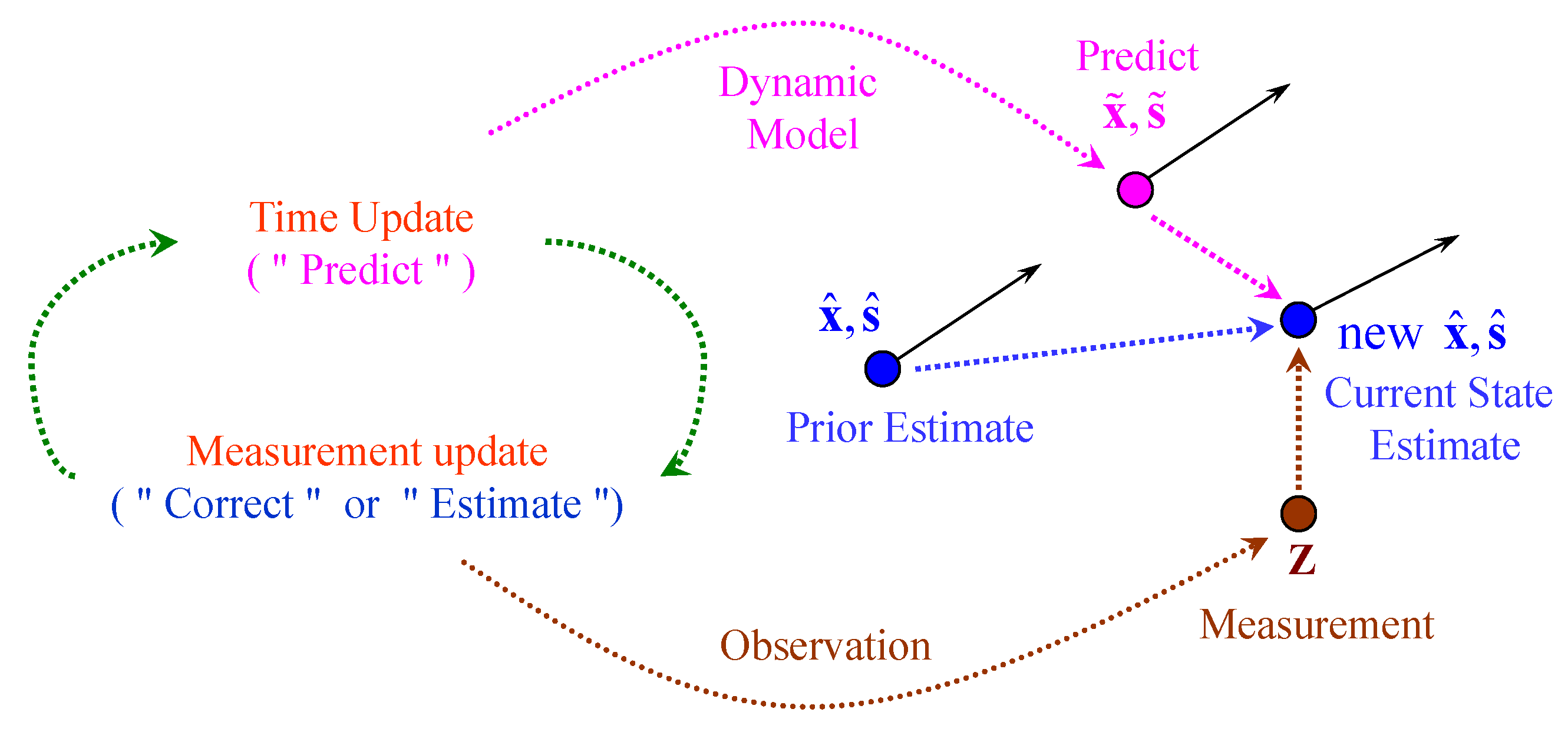
2. Kalman Filtering Algorithm
3. Alpha-Beta (α-β) Filtering Algorithm
- (1)
- Prediction step (Time update phase):
- (2)
- Estimation step (Measurement update phase):
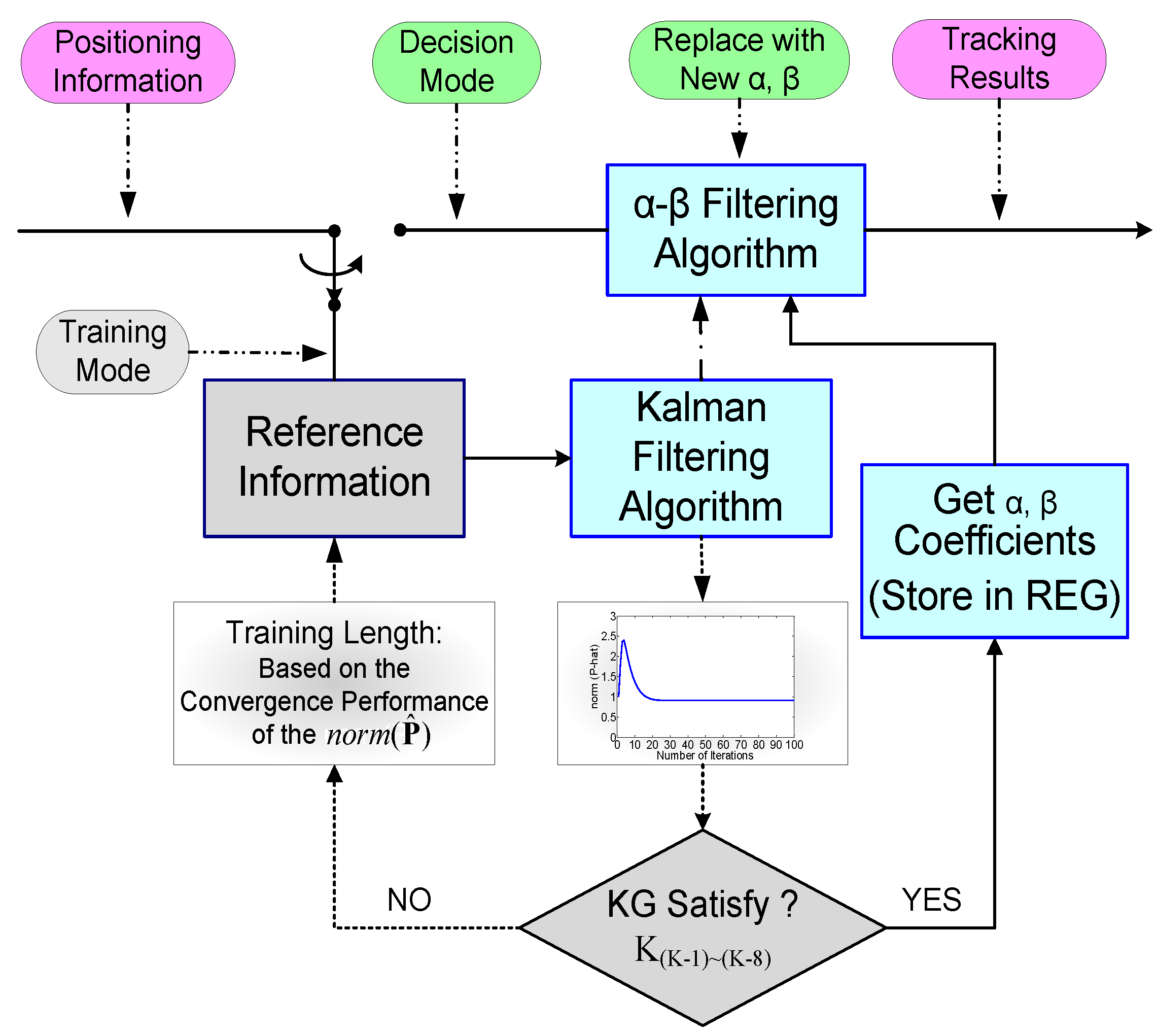
4. The Proposed Filtering Algorithm Based on Chip
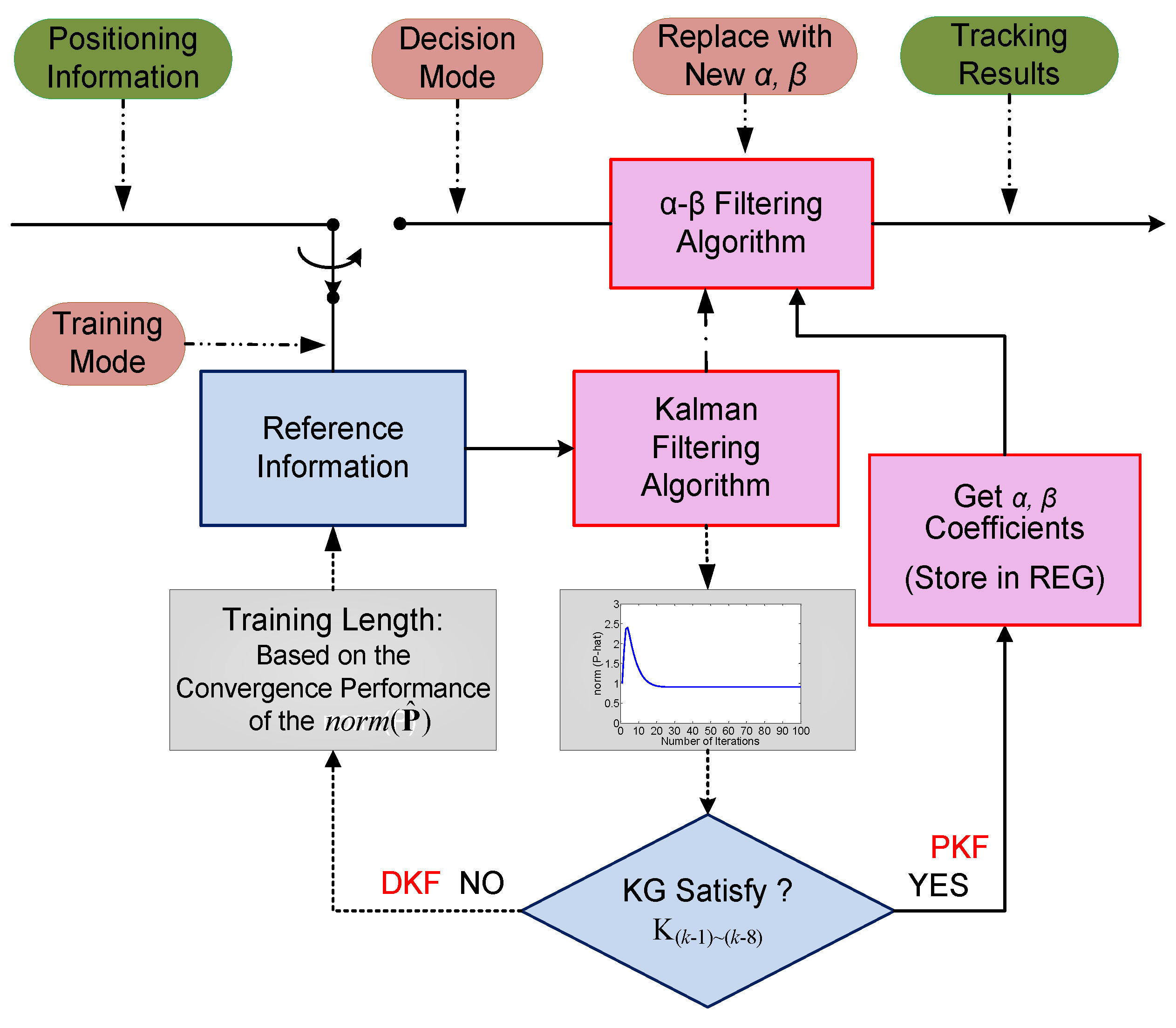
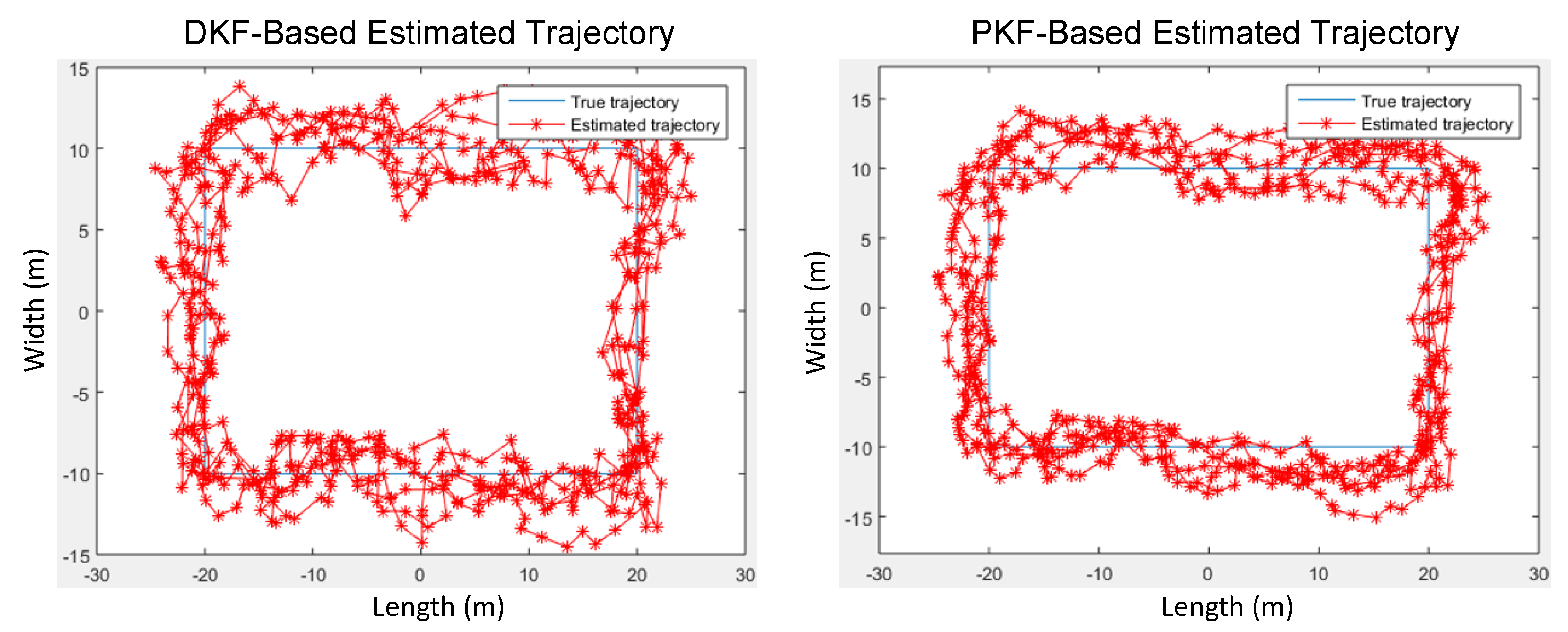
4.1. DKF and PKF Filtering Algorithm
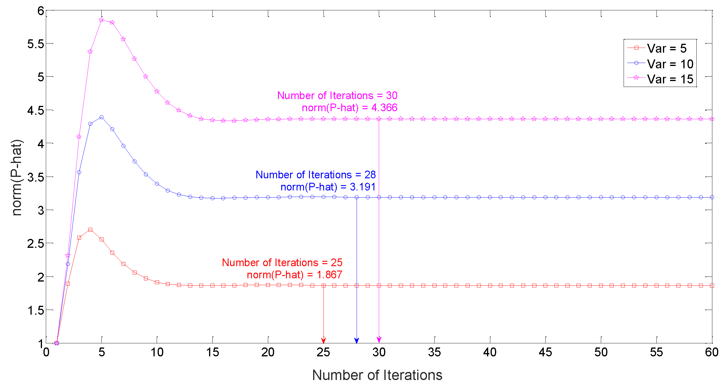
4.2. Revise Covariance R and Q in Different Environments
4.3. Judgment-Standard for Conditional Equation
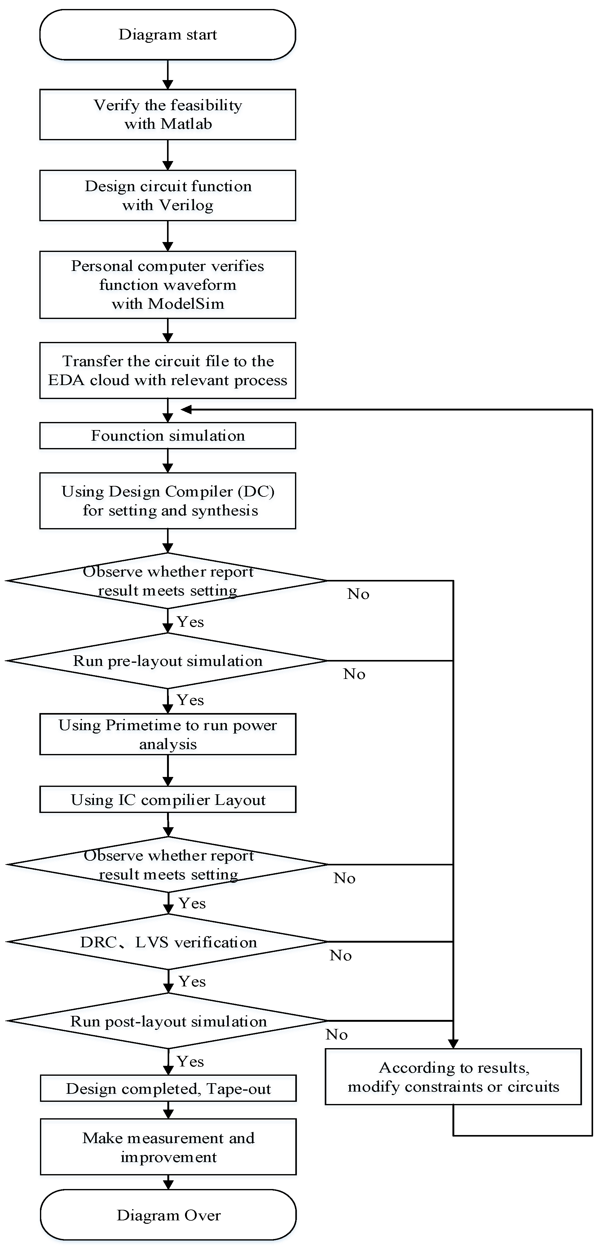
5. The Proposed VLSI Architecture and Implementation
5.1. The Algorithm Implementation and Pipeline Architecture
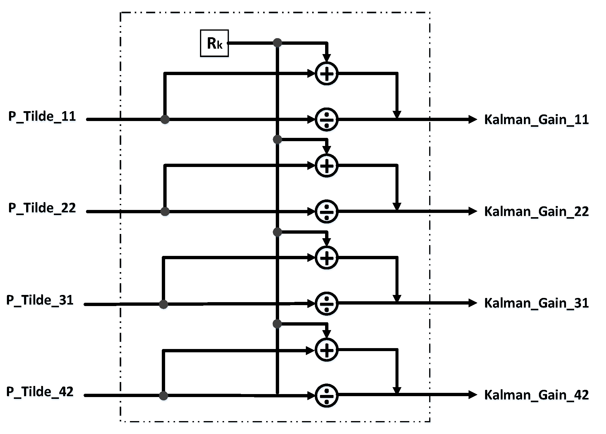
5.2. Computation of Kalman Gain and α-β Module
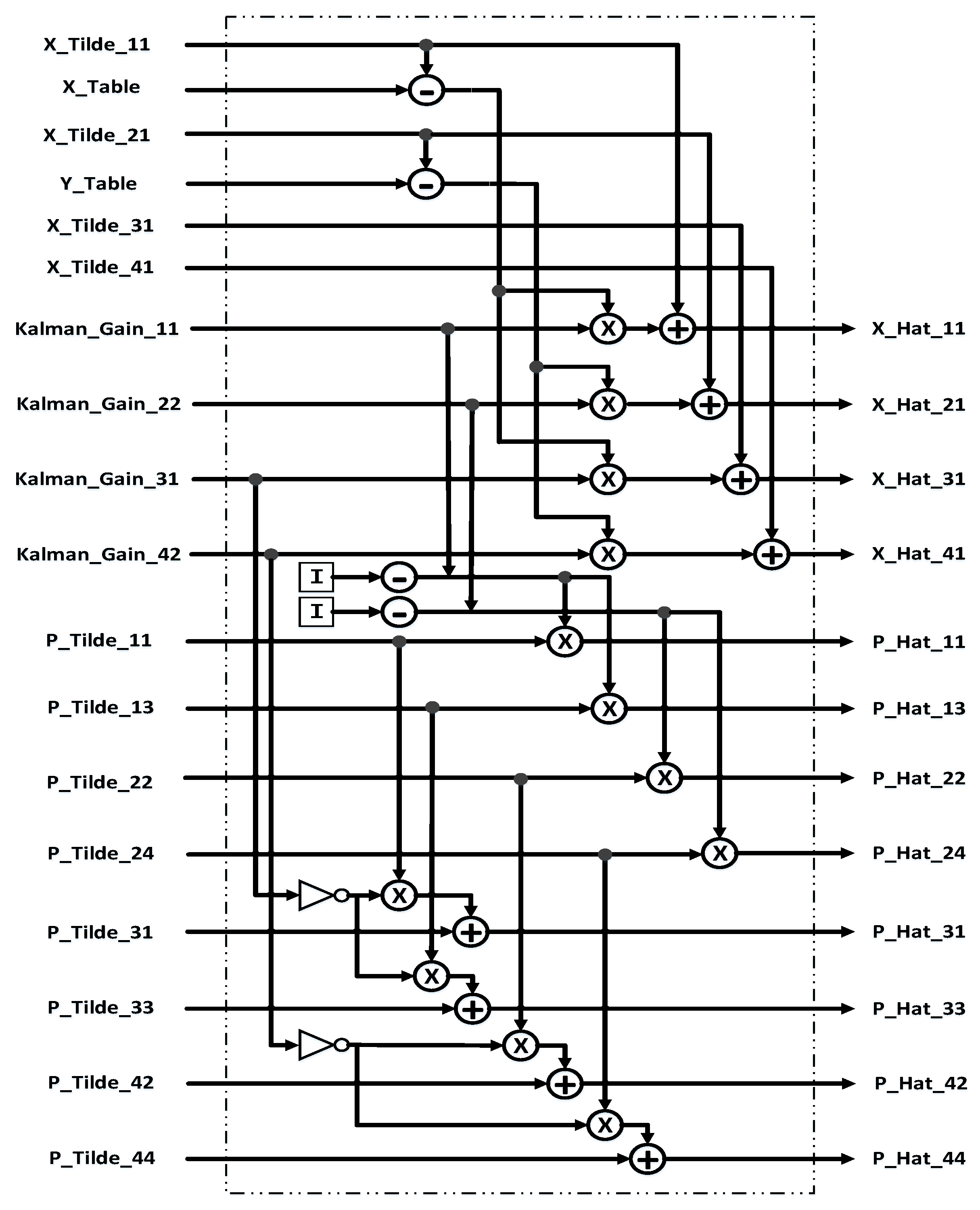
5.3. Update State Module
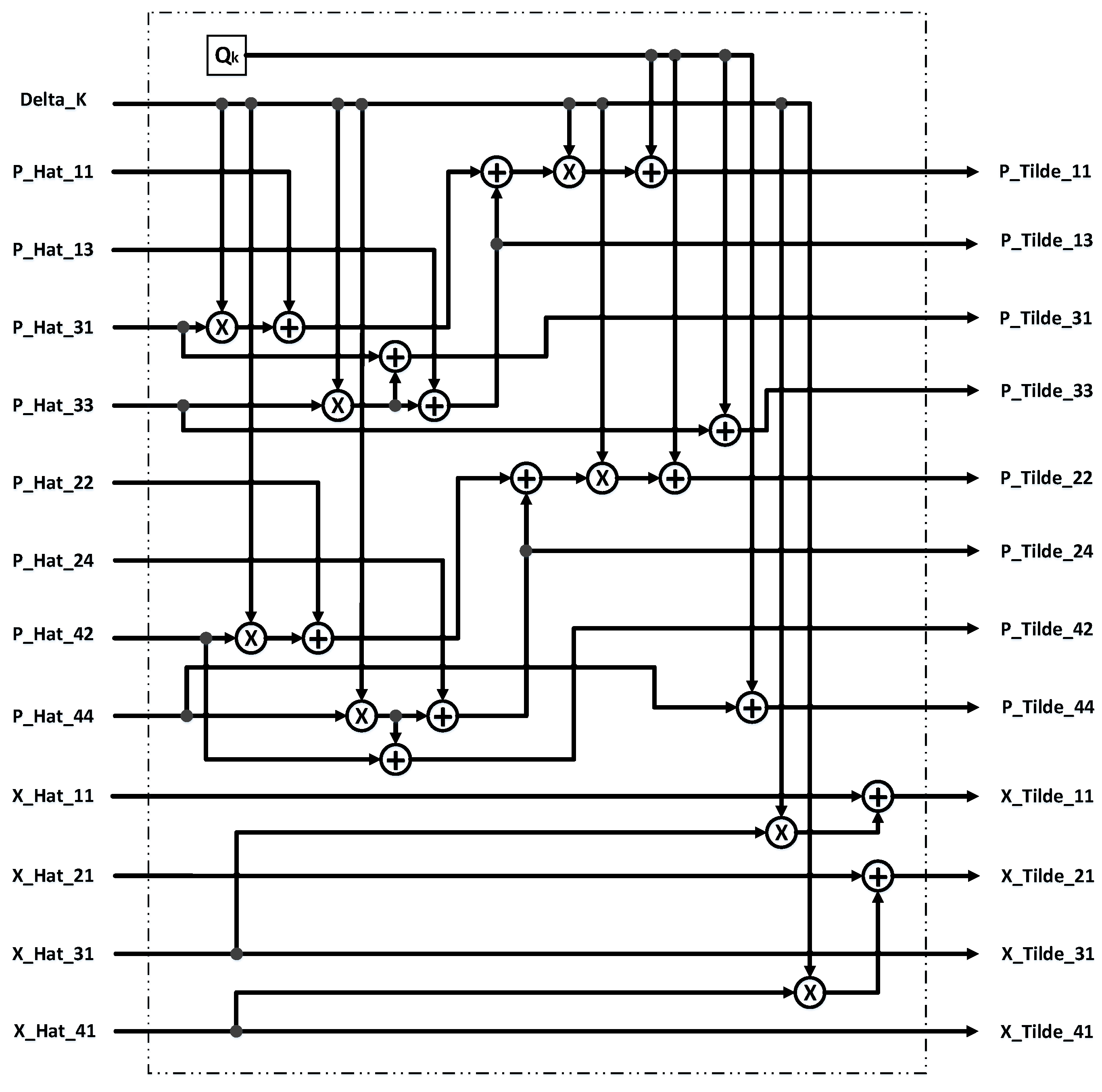
5.4. Predicted State Module
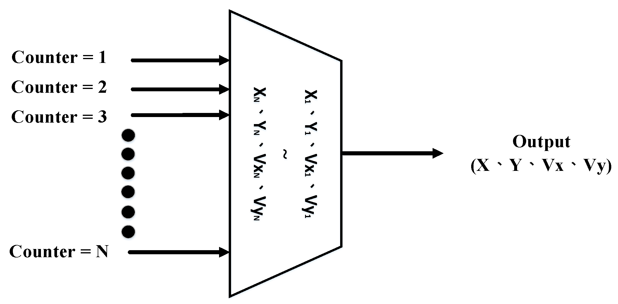
5.5. Input Table Module
6. The Implementation of Chip Results and Measurement
6.1. Data Comparison with FPGA Approach
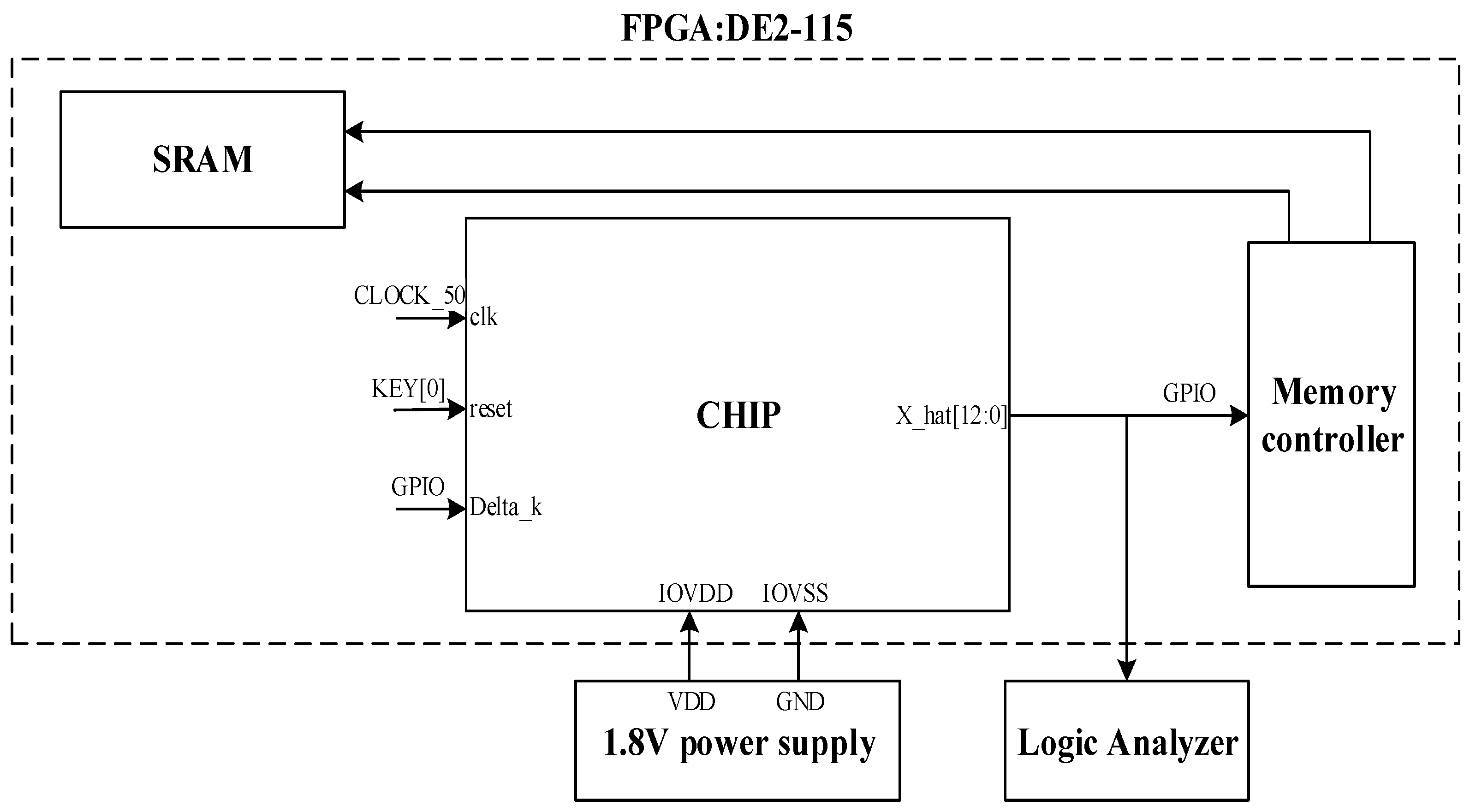
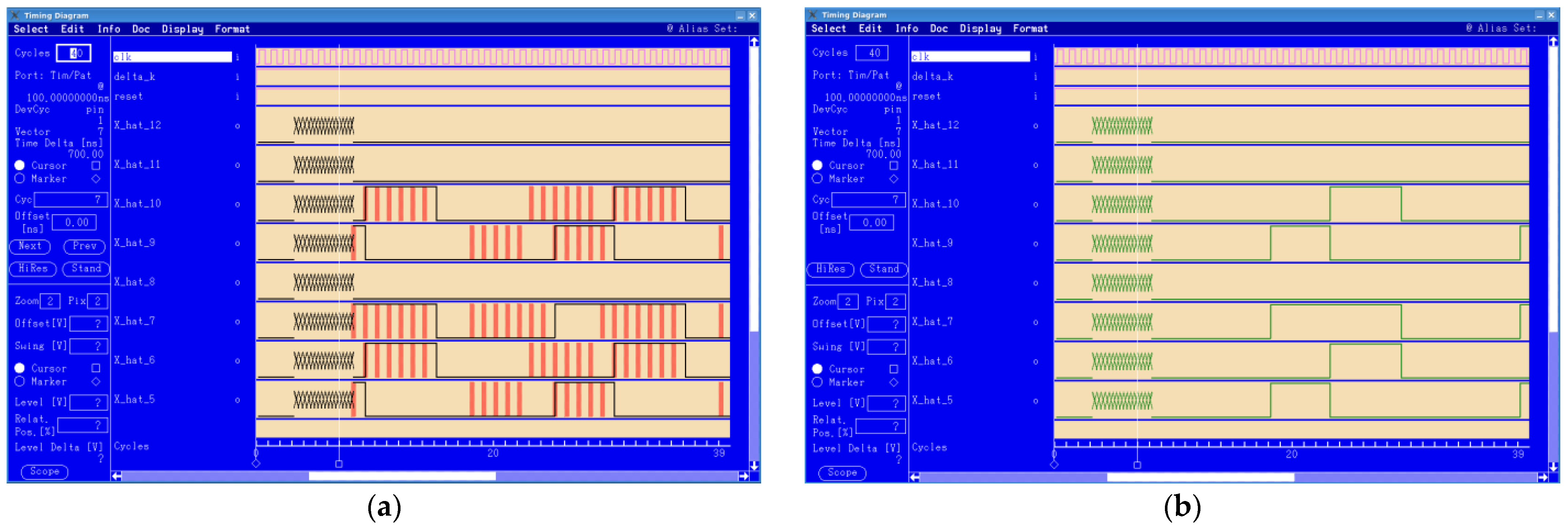
6.2. Simulation on FPGA DE2-115
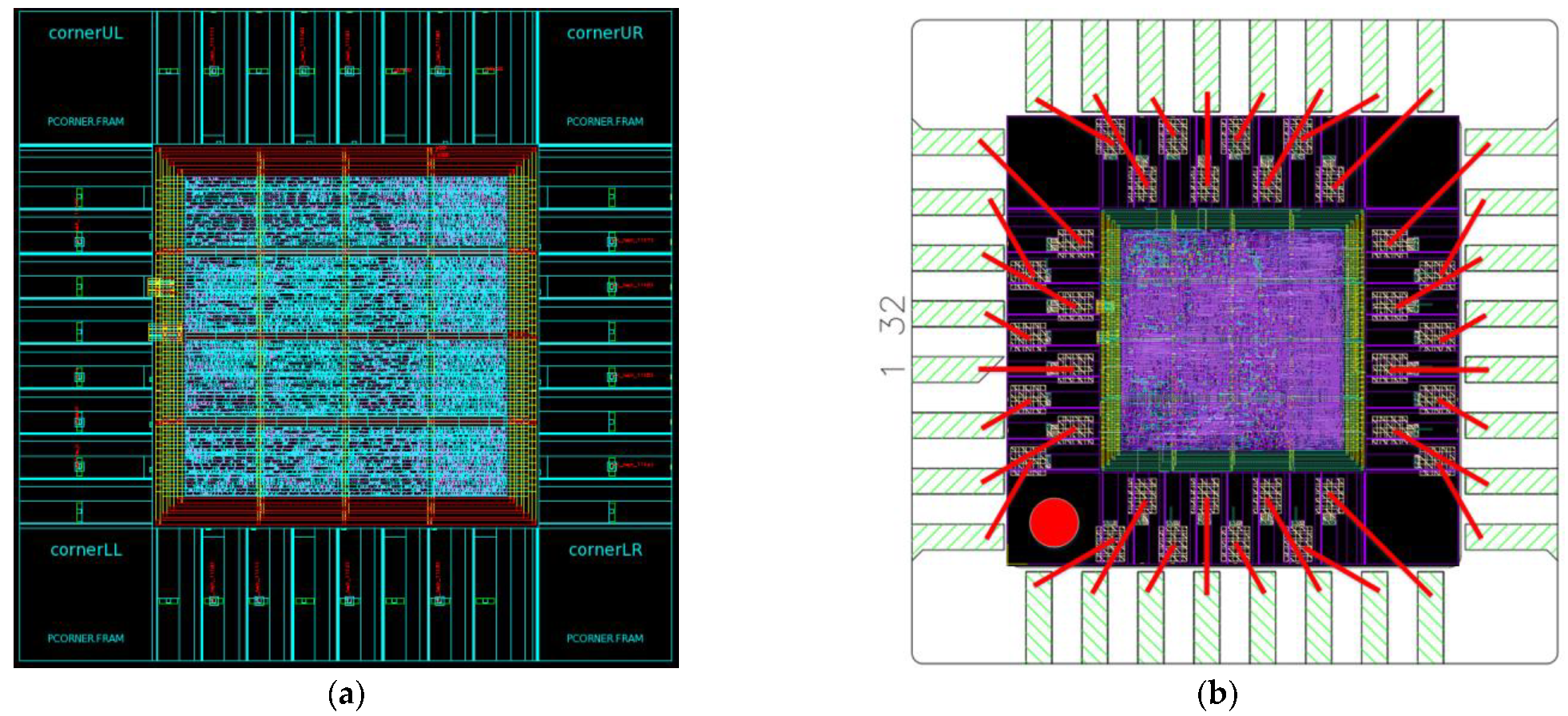
6.3. Implementation of Chip
6.4. Measurement of Chip
7. Conclusions
Author Contributions
Funding
Acknowledgments
Conflicts of Interest
References
- Akpakwu, G.A.; Silva, B.J.; Hancke, G.P.; Abu-Mahfouz, A.M. A survey on 5G networks for the Internet of Things: Communication technologies and challenges. IEEE Access 2018, 6, 3619–3647. [Google Scholar] [CrossRef]
- Zafari, F.; Papapanagiotou, I.; Christidis, K. Micro-location for Internet of Things equipped smart buildings. IEEE Internet Things J. 2016, 3, 96–112. [Google Scholar] [CrossRef]
- Mohammadi, M.; Al-Fuqaha, A.; Guizani, M.; Oh, J.-S. Semi-supervised deep reinforcement learning in support of IoT and smart city services. IEEE Internet Things J. 2018, 5, 624–635. [Google Scholar] [CrossRef]
- Chen, L.; Thombre, S.; Järvinen, K.; Lohan, E.S.; Alén-Savikko, A.; Leppäkoski, H. Robustness, security and privacy in location-based services for future IoT: A survey. IEEE Access 2017, 5, 8956–8977. [Google Scholar] [CrossRef]
- Lin, X.; Bergman, J.; Gunnarsson, F.; Liberg, O.; Razavi, S.M.; Razaghi, H.S.; Rydn, H.; Sui, Y. Positioning for the Internet of Things: A 3GPP Perspective. IEEE Commun. Mag. 2017, 55, 179–185. [Google Scholar] [CrossRef]
- Yeow, K.; Gani, A.; Ahmad, R.W.; Rodrigues, J.J.P.C.; Ko, K. Decentralized consensus for edge-centric Internet of Things: A review, taxonomy, and research issues. IEEE Access 2017, 18, 1–10. [Google Scholar] [CrossRef]
- Dardari, D.; Closas, P.; Djuric, P.M. Indoor tracking: Theory, methods, and technologies. IEEE Trans. Veh. Technol. 2015, 64, 1263–1278. [Google Scholar] [CrossRef]
- Enhanced 911-Wireless Services. Available online: https://www.fcc.gov/general/enhanced-9-1-1-wireless-services (accessed on 29 November 2022).
- Rantakokko, J.; Rydell, J.; Strömbäck, P.; Händel, P.; Callmer, J.; Törnqvist, D.; Gustafsson, F.; Jobs, M.; Grudén, M. Accurate and reliable soldier and first responder indoor positioning: Multisensor systems and cooperative localization. IEEE Wirel. Commun. 2011, 18, 10–18. [Google Scholar] [CrossRef]
- Chiou, Y.-S.; Tsai, F. A reduced-complexity data-fusion algorithm using belief propagation for location tracking in heterogeneous observations. IEEE Trans. Cybern. 2014, 44, 922–935. [Google Scholar] [CrossRef]
- What A Smart City is All About. Available online: https://standards.ieee.org/beyond-standards/what-a-smart-city-is-all-about/ (accessed on 15 January 2023).
- Yeh, S.-C.; Wang, C.-H.; Hsieh, C.-H.; Chiou, Y.-S.; Cheng, T.-P. Cost-Effective Fitting Model for Indoor Positioning Systems Based on Bluetooth Low Energy. Sensors 2022, 22, 6007. [Google Scholar] [CrossRef]
- Yeh, S.-C.; Lai, C.-J.; Tsai, F.; Chiou, Y.-S. Research on calibration-free fingerprinting positioning techniques based on terrestrial magnetism databases for indoor environments. IET Radar Sonar Navig. 2022, 16, 896–911. [Google Scholar] [CrossRef]
- Haykin, S. Kalman Filtering and Neural Networks, 1st ed.; John Wiley & Sons, Inc.: New York, NY, USA, 2004. [Google Scholar]
- Chiou, Y.-S.; Wang, C.-L.; Yeh, S.-C. An adaptive location estimator based on Kalman filtering for dynamic indoor environments. In Proceedings of the 64th IEEE Vehicular Technology Conference (IEEE VTC2006-Fall), Montreal, QC, Canada, 25–28 September 2006; pp. 25–28. [Google Scholar]
- Yang, H.; Yang, R.; Hu, W.; Huang, Z. FPGA-Based Sensorless Speed Control of PMSM Using Enhanced Performance Controller Based on the Reduced-Order EKF. IEEE J. Emerg. Sel. Top. Power Electron. 2019, 9, 289–301. [Google Scholar] [CrossRef]
- Soh, J.; Wu, X. An FPGA-Based Unscented Kalman Filter for System-On-Chip Applications. IEEE Trans. Circuits Syst. II Express Briefs 2016, 64, 447–451. [Google Scholar] [CrossRef]
- Chen, W.-T.; Chen, S.-L.; Chiou, Y.-S.; Lin, T.-L.; Wen, F.-J.; Lin, Y.-K. FPGA-based implementation of reduced-complexity filtering algorithm for real-time location tracking. In Proceedings of the 2019 IEEE Intl Conf on The 17th IEEE International Conference on Dependable, Autonomic and Secure Computing (DASC 2019), Fukuoka, Japan, 5–8 August 2019; pp. 721–726. [Google Scholar]
- Zhang, Y.S.; Chen, T.H.; Chiou, Y.S.; Chen, S.L.; Chen, W.T.; Lin, Y.K.; Wen, F.J.; Lin, T.L. Design and implementation of real-time localization algorithms based on FPGA for positioning and tracking. In Proceedings of the 2019 IEEE Eurasia Conference on IOT, Communication and Engineering (ECICE 2019), Yunlin, Taiwan, 3–6 October 2019; pp. 446–448. [Google Scholar]
- Bai, X.; Wang, D.-M.; Tu, J.-J.; Zhao, B.-H. The hardware design and simulation of Kalman filter based on IP core and time-sharing multiplex. In Proceedings of the 2011 International Conference on Intelligent Computation Technology and Automation (ICICTA 2011), Shenzhen, China, 28–29 March 2011; pp. 266–269. [Google Scholar]
- Jung, K.; Bermudez, P.B.V.; Hwang, H.; Oh, Y. Passenger’s location estimation using Kalman filter for Beacon fare collection in a wireless low floor tram. In Proceedings of the 2018 International Conference on Electronics, Information, and Communication (ICEIC 2018), Honolulu, HI, USA, 24–27 January 2018; pp. 1368–1373. [Google Scholar]
- Chiou, Y.-S.; Tsai, F.; Yeh, S.-C. A dead-reckoning positioning scheme using inertial sensing for location estimation. In Proceedings of the 2014 IEEE The Tenth International Conference on Intelligent Information Hiding and Multimedia Signal Processing (IIH-MSP 2014), Kitakyushu, Japan, 27–29 August 2014; pp. 377–380. [Google Scholar]
- Li, Q.; Li, R.; Ji, K.; Dai, W. Kalman filter and its application. In Proceedings of the 2015 8th International Conference on Intelligent Networks and Intelligent Systems (ICINIS 2015), Tianjin, China, 1–3 November 2015; pp. 74–77. [Google Scholar]
- Wang, S.; Feng, J.; Tse, C.K. Analysis of the Characteristic of the Kalman Gain for 1-D Chaotic Maps in Cubature Kalman Filter. IEEE Signal Process. Lett. 2013, 20, 229–232. [Google Scholar] [CrossRef]
- Jain, A.; Krishnamurthy, P.K. Phase Noise Tracking and Compensation in Coherent Optical Systems Using Kalman Filter. IEEE Commun. Lett. 2016, 20, 1072–1075. [Google Scholar] [CrossRef]
- Medeiros, H.; Park, J.; Kak, A. Distributed Object Tracking Using a Cluster-Based Kalman Filter in Wireless Camera Networks. IEEE J. Sel. Top. Signal Process. 2008, 2, 448–463. [Google Scholar] [CrossRef]
- Zheng, J.; Alam Bhuiyan, Z.; Liang, S.; Xing, X.; Wang, G. Auction-based adaptive sensor activation algorithm for target tracking in wireless sensor networks. Futur. Gener. Comput. Syst. 2014, 39, 88–99. [Google Scholar] [CrossRef]
- Wang, X.; Fu, M.; Zhang, H. Target Tracking in Wireless Sensor Networks Based on the Combination of KF and MLE Using Distance Measurements. IEEE Trans. Mob. Comput. 2011, 11, 567–576. [Google Scholar] [CrossRef]
- Yu, K.K.C.; Watson, N.R.; Arrillaga, J. An Adaptive Kalman Filter for Dynamic Harmonic State Estimation and Harmonic Injection Tracking. IEEE Trans. Power Deliv. 2005, 20, 1577–1584. [Google Scholar] [CrossRef]
- Chiou, Y.-S.; Tsai, F.; Wang, C.-L.; Huang, C.-T. A reduced-complexity scheme using message passing for location tracking. EURASIP J. Adv. Signal Process. 2013, 44, 922–935. [Google Scholar] [CrossRef]
- Wang, C.-L.; Chiou, Y.-S.; Dai, Y.-S. An adaptive location estimator based on alpha-beta filtering for wireless sensor networks. In Proceedings of the 2007 IEEE Wireless Communications and Networking Conference (WCNC 2007), Hong Kong, China, 11–15 March 2007; pp. 3285–3290. [Google Scholar]
- Chiou, Y.-S.; Wang, C.-L.; Yeh, S.-C. Reduced-complexity scheme using alpha–beta filtering for location tracking. IET Commun. 2011, 5, 1806–1813. [Google Scholar] [CrossRef]
- Yoo, K.; Chun, J.; Shin, J. Target tracking; classification for missile using interacting multiple model (IMM). In Proceedings of the 2018 IEEE International Conference on Radar (RADAR 2018), Brisbane, QLD, Australia, 27–31 August 2018; pp. 1–6. [Google Scholar]
- Aly, S.M.; El Fouly, R.; Braka, H. Extended Kalman filtering and interacting multiple model for tracking maneuvering targets in sensor netwotrks. In Proceedings of the 2009 IEEE Intelligent Solutions in Embedded Systems, Ancona, Italy, 25–26 June 2009; pp. 149–156. [Google Scholar]
- Rico-Aniles, H.D.; Ramirez-Cortes, J.M.; Rangel-Magdaleno, J.J. FPGA-based matrix inversion using an iterative chebyshev-type method in the context of compressed sensing. In Proceedings of the 2014 IEEE International Instrumentation and Measurement Technology Conference (I2MTC 2014), Montevideo, Uruguay, 12–15 May 2014; pp. 983–987. [Google Scholar]
- Kalman Filter in One Dimension. Available online: https://www.kalmanfilter.net/kalman1d.html (accessed on 15 January 2023).
- Rawal, N. HDL implementation of Kalman filter for GNSS receiver. In Proceedings of the 2015 International Advance Computing Conference (IACC 2015), Banglore, India, 12–13 June 2015; pp. 266–269. [Google Scholar]


| DKF (Difference Kalman Filter) | PKF (Percentage Kalman Filter) | |
|---|---|---|
| Method of judgment | Using differences to make judgment | Using percentages to make judgment |
| Using situation | Smaller KG in the environment | Larger KG in the environment |
| Variance V | Steady KG of KF | KG of 4.0/ Iteration Times | KG of 8.0/ Iteration Times | KG of 16.0/ Iteration Times | KG of 32.0/ Iteration Times |
|---|---|---|---|---|---|
| 5 | 5830 | 5830/26 | 5830/25 | 5830/22 | 5826/21 |
| 10 | 5053 | 5053/29 | 5053/28 | 5053/23 | 5013/20 |
| 15 | 4638 | 4638/32 | 4638/30 | 4638/24 | 4584/19 |
| Number of Slice Registers | Number of Slice LUTs | Number of IOBs | Processing Time (One Clock) | |
|---|---|---|---|---|
| Bai’s Approach [20] | 36,689/149,760 (24%) | 28,367/149,760 (18%) | 391/680 (57%) | 0.00468 ns |
| Rawal’s Approach [37] | 2696/393,600 (1%) | 17,335/196,800 (8%) | 166/600 (27%) | - |
| The Proposed Approach | 8739/114,480 (8%) | 9365/117,053 (8%) | 102/529 (19%) | 0.003007 ns |
| Logic Element Usage by Number of LUT Inputs | Total Registers | Total I/O Pins | Embedded Multiplier 9-Bit Elements | |
|---|---|---|---|---|
| Chen’s Approach [18] | 18,650/114,480 (16%) | 2178 | 120/529 (23%) | 192/532 (36%) |
| Zhang’s Approach [18,19] | 22,176/114,480 (20%) | 1687 | 102/529 (19%) | 144/532 (27%) |
| The Proposed Approach | 8739/114,480 (8 %) | 929 | 102/529 (19%) | 60/532 (11%) |
| Processing Time (One Clock) | Stage | Points | Cycles | Total Processing Time (One Cycle) | |
|---|---|---|---|---|---|
| Chen’s Approach [18] | 0.002772 ns | 6 | 1800 | 10,800 | 29.9376 ns |
| Zhang’s Approach [18,19] | 0.002800 ns | 6 | 1800 | 10,800 | 30.2400 ns |
| The Proposed Approach | 0.003007 ns | 4 | 1800 | 1804 | 5.4246 ns |
| Traditional Software Program (CPU i3/Ram 8 GB) | Traditional Software Program (CPU i7/Ram 16 GB) | The Proposed Approach (Hardware Design and FPGA) | ||||
|---|---|---|---|---|---|---|
| Algorithm | KF | α-β | KF | α-β | KF | α-β |
| Executing Time | 0.8235 ns | 0.07358 ns | 0.05115 ns | 0.009521 ns | 0.03407 ns | 0.003007 ns |
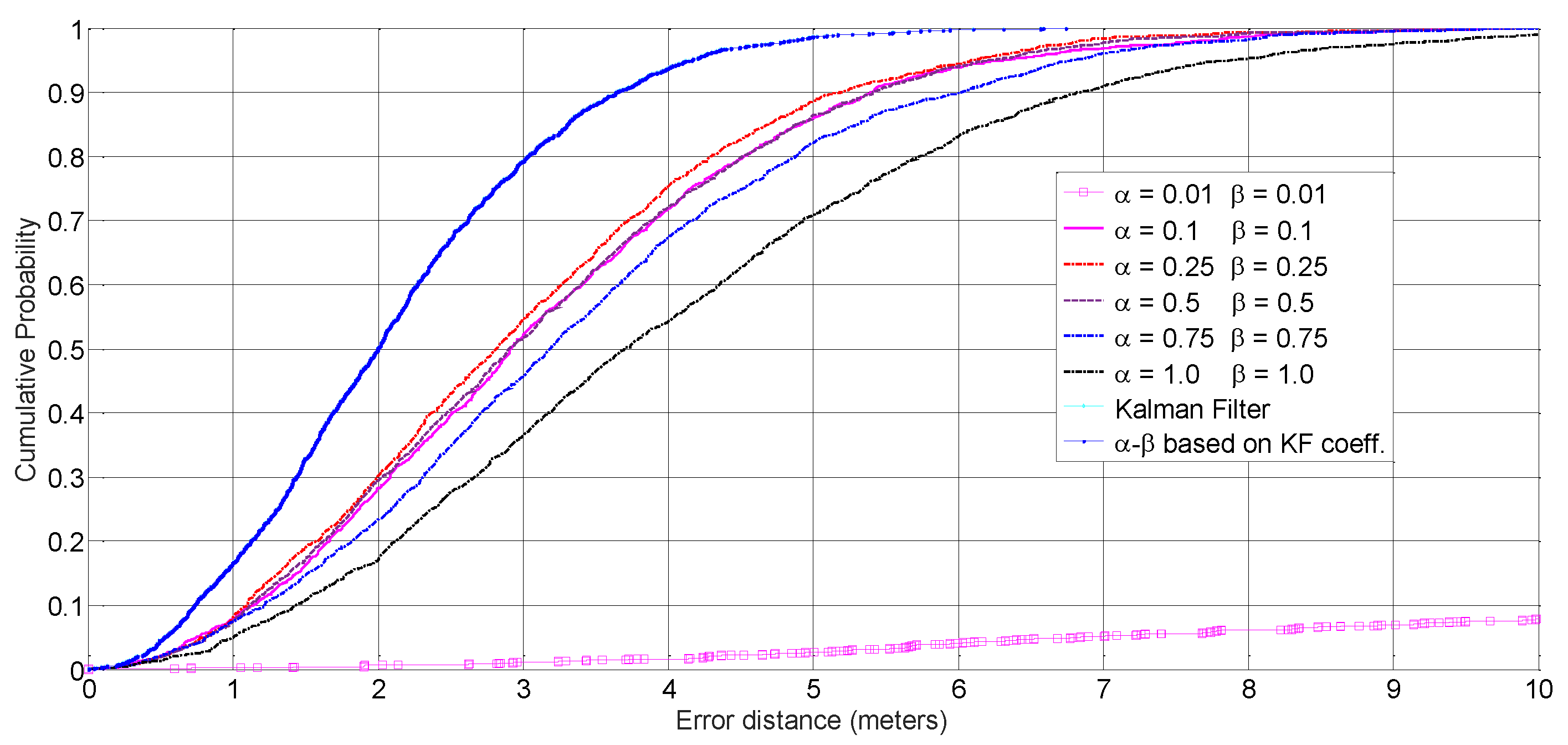
| Method | KF Approach | α-β Approach Based on KF Coeff. | α-β Approach α= 1 β = 1 | α-β Approach α= 0.75 β = 0.75 | α-β Approach α= 0.5 β = 0.5 | α-β Approach α= 0.25 β = 0.25 | |
|---|---|---|---|---|---|---|---|
| CDF | |||||||
| 90% | 3.65 m | 3.66 m | 6.82 m | 6.02 m | 5.42 m | 5.21 m | |
| 50% | 2.00 m | 2.01 m | 3.71 m | 3.19 m | 2.92 m | 2.81 m | |
| Specification | Spec. |
|---|---|
| Technology | TSMC 0.18 um CMOS Mixed Signal RF General Purpose Standard Process FSG AI 1P6M1.8&3.3 V |
| Process (μm) | 0.18 |
| Gate Counts | 22.84 k |
| Frequency (Hz) | 83.33 M |
| Chip Size (μm2) | 582.63 × 580.23 |
| Power Supply (Volts) | 1.8 |
| Operation Temperature (°C) | 0~125 |
| Power Consumption (W) | 3.86 m |
| Packing Type | 32 S/B |
| Chip Pads | GPIO |
|---|---|
| Clk | [0] |
| Reset | [4] |
| Delta_k | [8] |
| X_Hat[12:0] | [11, 13, 15, 17, 19, 21, 23, 25, 27, 29, 31, 33, 35] |
Disclaimer/Publisher’s Note: The statements, opinions and data contained in all publications are solely those of the individual author(s) and contributor(s) and not of MDPI and/or the editor(s). MDPI and/or the editor(s) disclaim responsibility for any injury to people or property resulting from any ideas, methods, instructions or products referred to in the content. |
© 2023 by the authors. Licensee MDPI, Basel, Switzerland. This article is an open access article distributed under the terms and conditions of the Creative Commons Attribution (CC BY) license (https://creativecommons.org/licenses/by/4.0/).
Share and Cite
Chiou, Y.-S.; Chen, S.-L.; Chen, W.-T. Reduced-Complexity Tracking Algorithms on Chip for Real-Time Location Estimation. Electronics 2023, 12, 739. https://doi.org/10.3390/electronics12030739
Chiou Y-S, Chen S-L, Chen W-T. Reduced-Complexity Tracking Algorithms on Chip for Real-Time Location Estimation. Electronics. 2023; 12(3):739. https://doi.org/10.3390/electronics12030739
Chicago/Turabian StyleChiou, Yih-Shyh, Shih-Lun Chen, and Wei-Ting Chen. 2023. "Reduced-Complexity Tracking Algorithms on Chip for Real-Time Location Estimation" Electronics 12, no. 3: 739. https://doi.org/10.3390/electronics12030739