SRFPI-LADRC Based Control Strategy for Off-Grid Single-Phase Inverter: Design, Analysis, and Verification

Abstract

Linear active disturbance rejection control (LADRC) has been extensively used in various areas due to its excellent disturbance suppression capability. When LADRC is applied to a single-phase inverter for tracking a sinusoidal reference signal, there is an inherent tracking inaccuracy problem. The steady-state error can be removed with the synchronous reference frame proportional-integral (SRFPI) control, which generates two orthogonal signals. In this paper, a modified control method based on compound SRFPI and LADRC for an off-grid single-phase inverter is put forward, where both output signals of SRFPI are employed as the reference signals of LADRC. Furthermore, a selective harmonic compensation method is performed by paralleling multiple SRFPI controllers to further reduce the selective harmonic components. Detailed theoretical analyses including system stability, robustness, performance of voltage tracking error and disturbance rejection are presented, which indicate that this organic combination fuses the merits of both SRFPI and LADRC without complicating the control design. Additionally, contrast experiments are conducted to demonstrate its effectiveness and superiority. These findings demonstrate that the system realizes a slight voltage tracking error and steady-state error, rapid dynamic response, and low total harmonic distortion (THD), especially under highly nonlinear load conditions.

1. Introduction

Single-phase inverters are applied frequently in renewable energy generation and all kinds of industrial fields. In general, the off-grid power generation and the power equipment, including the uninterrupted power supply (UPS) and the outdoor power supply, heavily rely on the single-phase inverters in a stand-alone mode [1,2,3]. High-performance single-phase inverters should provide a stable and high-quality sinusoidal voltage that possesses rapid dynamic performance, minor steady-state error, and small THD [4]. To achieve high performances of the inverters, breakthroughs can be made from power devices, circuit topology as well as control strategies [5,6]. In recent years, the proper control methods applied to inverters have increasingly grown in importance in the power electronics field.

In a voltage-source inverter system, the non-ideal factors, such as parasitic parameters, model parameter mismatch, and sampling noise, may cause the deterioration of the output voltage. Traditional single or dual closed-loop control methods with the proportional-integral-derivative (PID) regulators have difficulty realizing a satisfactory performance. The estimation and compensation of uncertainty/disturbance have received a lot of attention in observer-based design during the past few decades, as reviewed in [7]. It enables the control structure with two degrees of freedom (2DOF), one of which is used to regulate the tracking performance and the other to compensate for the uncertainty/disturbance [8]. The disturbance estimation techniques, such as the disturbance observer [9], the uncertain disturbance estimator [10] and the extended state observer (ESO) in active disturbance rejection control (ADRC) [11], have been successfully applied in different fields, including three-phase inverter [12] and single-phase inverter systems [13]. As a fundamental part of ADRC, the ESO estimates the generalized disturbances, which lump together both unknown dynamics and disturbance, and only requires consideration of the system’s relative degree instead of the accurate model [7]. Then, ADRC performs dynamic compensation through the feedback control [14]. Thus, reference tracking and disturbance rejection can be achieved simultaneously. Nonlinear functions in ADRC increase the complexity of parameter tuning. Aiming at this problem, Z. Gao proposed the linear ADRC (LADRC) method, which employs a linear ESO (LESO) and a linear error feedback control law. In this way, the control parameters are reduced to two; namely, the controller bandwidth and the observer bandwidth [15]. Meanwhile, analyses can be performed using the frequency domain technique, which is frequently used in engineering. The LADRC is now more feasible in practice due to all these initiatives.

Real-time disturbance compensation ensures good dynamic performance with LADRC. However, the LESO is unable to accurately estimate the quickly varying sinusoidal disturbance, so the conventional LADRC is unable to track the sinusoidal signal without error [16]. The significant tracking error and voltage THD limit the use of LADRC in a single-phase inverter system. By adding additional controllers such as the proportional-resonant controller, the repetitive controller, and other controllers, LADRC-based compound control offers an intuitive method for improvement. By choosing a resonant frequency equal to the reference frequency, the proportional-resonant controller can track the sinusoidal signal well. However, it is susceptible to a phase shift of the detected signals, which may cause high sensitivity and instability [17]. Although RC has a great harmonic cancellation capability, its low dynamic response restricts its application [18].

The synchronous reference frame proportional-integral (SRFPI) controller is adopted far and wide in three-phase converter systems due to its ability to suppress the periodic disturbances. It is becoming more prevalent in single-phase inverter applications [19,20,21]. To utilize SRFPI, a fictitious orthogonal voltage signal needs to be produced with the orthogonal-signal-generation (OSG) method. Then, the ac signals in the α-β static reference frame are converted to dc signals in the synchronous reference frame (SRF). PI regulators are subsequently used to remove the steady-state error [19]. However, SRFPI has a poor ability to suppress non-periodic disturbances. A harmonic compensator (HC) consisting of multi-SRFPI controllers is proposed in [20,21], which can prevent low-order harmonics, particularly under nonlinear loads.

In our earlier work, to combine the advantages of SRFPI and LADRC, a novel single-phase inverter control technique based on cascade connected SRFPI and LADRC [22] is developed, where the first output signal of SRFPI is taken as the voltage reference of LADRC. Prompted by the fact that the SRFPI, which outputs two orthogonal signals, naturally provides a voltage reference and a differential voltage reference, the second output signal of SRFPI is utilized as the differential voltage reference of LADRC to further improve the system performance in [23].

Table 1. Feature comparison of single-phase inverters with different control methods.

Comparative Item	Single/Dual-Loop PID Control	SRFPI Control	LADRC	SRFPI-LADRC
System robustness	Medium	Medium	Good	Good
Steady-state performance	Medium	Good	Medium	Good
Transient performance	Medium	Good	Good	Good
Virtual orthogonal signals	Not required	Required	Not required	Required
Hardware cost	Low	Low	Low	Medium

explicates the feature comparison of the single/dual-loop PID control, SRFPI control, LADRC, and SRFPI-LADRC for single-phase inverters, which demonstrates the performance superiority of the suggested strategy.

Remark: Ref. [23] is a conference paper, where we briefly discussed the implementation of LADRC and the modeling of SRPFI-LADRC and provided contrast simulation results. In this paper, the SRFPI-LADRC-based compound control method in [23] is further studied and optimized, including more in-depth theoretical explanations, a harmonic suppression technique and sufficient experimental verifications.

The main contributions of this work are as follows:

(1)

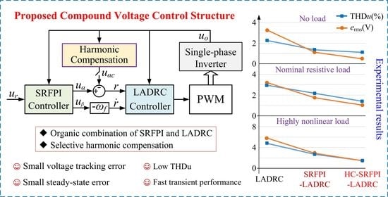
The benefits of introducing a differential reference into LADRC is analyzed. Detailed theoretical analyses of the SRFPI-LADRC-based strategy, including system stability, robustness, performance of the voltage tracking error and disturbance rejection are presented, which indicate that the organic combination of SRFPI and LADRC fuses the merits of both without adding complexity to the parameters design.

(2)

The HC, consisting of paralleled multiple SRFPI controllers corresponding to harmonic frequencies, is built to remove the selective harmonic components. The HC also enhances the performance of the disturbance rejection.

(3)

Contrast experiments are conducted, and the findings verify that the proposed method significantly improves the system performance in terms of the tracking error and steady-error, dynamic response, and voltage THD (THDu).

This paper is organized as follows. Section 2 introduces the design of the LADRC-based voltage controller. The proposed compound control technique is discussed in Section 3, along with the pertinent theoretical analysis. The HC is shown in Section 4. Discussion of the experimental results appears in Section 5. Finally, Section 6 concludes this paper.

2. Design of LADRC for Single-Phase Inverter

2.1. Modeling of Single-Phase Inverter

Figure 1 depicts a full-bridge inverter’s usual configuration. L and C are the filter-parameters; r_e is the inductor’s equivalent series resistance (ESR); i_o is the output current and i_L is the inductor current; U_dc denotes the dc-link voltage; and u_in and u_o are the input and output voltage, respectively. This work investigates the resistive load R and the nonlinear load. Specifically, the nonlinear load is made up of a resistor R_s and a diode rectifier bridge that feeds a capacitor C_z in parallel with a resistor R_z.

The equivalent model of the single-phase inverter is shown in Figure 2. K_PWM is the equivalent gain of H-bridge, and its value is equal to U_dc. To make the model simpler, a proportional gain 1/U_dc is coupled in series with the control signal u(s), where u_m(s) is the sinusoidal modulation signal.

Taking i_o into account as the input disturbance, the plant’s transfer function can be described as

$$G_p(s)=\frac{u_o(s)}{u_{in}(s)}=\frac{u_o(s)}{u(s)}=\frac{1}{LC{s}^2+r_{e}Cs+1}$$

(1)

According to Equation (1), the differential form of the inverter can be expressed as

$${\ddot{u}}_o=-a_1{\dot{u}}_o-a_0{u}_o+b_{0}u$$

(2)

where a₀ = 1/LC, a₁ = r_e/L, and b₀ = 1/LC.

2.2. Design of LADRC

Observing Equation (2), it can be seen the plant is not a standard series-integral system. To compensate the inverter system into a series-integral type, the different part is regarded as the known disturbance f₀:

$$f_0=-a_1{\dot{u}}_o-a_0{u}_o$$

(3)

Note that the differential Equation (2) ignores the effects of the parameter perturbation, unmodeled part, sampling noise, etc. These parts are treated as the unknown disturbance f₁. Then, the total disturbance can be defined as f = f₁ + f₀. Thus, the single-phase inverter system with an LC filter can be rewritten in the LADRC framework as

$${\ddot{x}}_1=b_{0}u+f$$

(4)

where x₁ = u_o is the output voltage of inverter.

The main idea of LADRC is to build a LESO that provides an estimated total disturbance $\widehat{f}$. Since f₁ is unavailable in practice, the LESO is implemented with the assumption that f₁ is differentiable and ${\dot{f}}_1$ is bounded [24]. The introduction of the known information in the design of LESO helps to reduce the uncertainty and improve the observation accuracy [11]. Let x₂ = ${\dot{u}}_o$, x₃ = f, x = [x₁ x₂ x₃]^T, and y = u_o. Taking the total disturbance f as the extended state variable, the inverter system in Equation (4) can be reformulated as the extended state-space representation:

$$\left\{\begin{array}{l}\dot{\mathit{x}}={\mathit{A}}_{\mathit{p}}x+{\mathit{B}}_{\mathit{p}}u+{\mathit{E}}_{\mathit{p}}{\dot{f}}_1\\ y={\mathit{C}}_{\mathit{p}}x\end{array}\right.$$

(5)

where

$${\mathit{A}}_{\mathit{p}}=\left[\begin{array}{ccc}0& 1& 0\\ 0& 0& 1\\ 0& -a_0& -a_1\end{array}\right],{\mathit{B}}_{\mathit{p}}=\left[\begin{array}{c}0\\ b_0\\ -a_1{b}_0\end{array}\right],{\mathit{E}}_{\mathit{p}}=\left[\begin{array}{c}0\\ 0\\ 1\end{array}\right],{\mathit{C}}_{\mathit{p}}=\left[\begin{array}{ccc}1& 0& 0\end{array}\right]$$

It can be seen that the known model parameters (a₀, a₁) are contained in the system matrix A_p.

Thus, the corresponding model-assisted LESO can be created as

$$\left\{\begin{array}{l}\dot{\mathit{z}}={\mathit{A}}_{\mathit{p}}\mathit{z}+{\mathit{B}}_{\mathit{p}}u+{\mathit{L}}_{\mathit{p}}(y-\widehat{y}) =({\mathit{A}}_{\mathit{p}}-{\mathit{L}}_{\mathit{p}}{\mathit{C}}_{\mathit{p}})\mathit{z}+{\mathit{B}}_{\mathit{p}}u+{\mathit{L}}_{\mathit{p}}y\\ \widehat{y}={\mathit{C}}_{\mathit{p}}\mathit{z}\end{array}\right.$$

(6)

where, z = [z₁ z₂ z₃]^T = [${\widehat{x}}_1$ ${\widehat{x}}_2$ ${\widehat{x}}_3$]^T = [${\widehat{u}}_o$ ${\widehat{\dot{u}}}_o$ $\widehat{f}$]^T represents the estimates of x₁, x₂ and x₃, and L_p = [l₁ l₂ l₃]^T denotes the error feedback gain matrix of the LESO. The decay rate of the observed error is determined by the eigenvalues of (A_p − L_pC_p), which are placed in the same location according to the popular bandwidth parametrization method [13]:

$$\lambda (s)=\left|s\mathit{I}-{\mathit{A}}_{\mathit{p}}+{\mathit{L}}_{\mathit{p}}{\mathit{C}}_{\mathit{p}}\right|={\left(s+{\omega }_o\right)}^3$$

(7)

where ω_o is the bandwidth of the observer. Thus,

$$\left\{\begin{array}{l}{l}_1=3{\omega }_o-a_1\\ l_2=3{\omega }_o^2-3a_1{\omega }_o-a_0+a_1^2\\ l_3={\omega }_o^3-3a_1{\omega }_o^2+3(a_1^2-a_0){\omega }_o+2a_0{a}_1-a_1^3\end{array}\right.$$

A real-time estimate of the variables is achieved via LESO. Ulteriorly, the control signal u and the feedback control law u_c for the system are designed as

$$\left\{\begin{array}{l}{u}_c=k_1(r-z_1)+k_2(\dot{r}-z_2)\\ u=(u_c-z_3)/b_0\end{array}\right.$$

(8)

where r is the reference signal of LADRC, and k₁ and k₂ are the proportional coefficients. According to the bandwidth tuning method [15], let k₁ = ${\omega }_c^2$, k₂ = 2ω_c, where ω_c represents the controller bandwidth of LADRC.

Substituting the control signal u into Equation (4), it can be seen that the system becomes a standard series-integral type:

$${\ddot{u}}_o=k_1(r-z_1)+k_2(\dot{r}-z_2)-z_3+f\approx u_c$$

(9)

Based on the above analysis, the LADRC-based control block schematic can be shown in Figure 3, which includes the LESO, the disturbance compensation block, and the error feedback control law. e = r − u_o denotes the tracking error. According to Equation (9), its transfer function can be derived as

$$e(s)=\frac{s^2}{s^2+2{\omega }_{c}s+{\omega }_c^2}r(s)$$

(10)

The bode magnitude plots of the tracking error transfer function with and without differential reference is compared, as shown in Figure 4. Notice that the introduction of the differential reference helps to improve the voltage tracking performance. However, because the unknown periodic disturbances such as the changing loads and the observation errors of LESO still exist, the system cannot be accurately compensated. Thus, a non-negligible steady-state error and THDu still exist when a fixed differential reference is given.

3. Design and Analysis of SRFPI-LADRC

As mentioned, the single-phase inverter using LADRC is infected by tracking errors. Aiming at this issue, a compound control method based on SRFPI and LADRC (SRFPI-LADRC) is proposed as displayed in Figure 5 [23], where the two orthogonal signals output by SRFPI naturally provide a voltage reference and a differential voltage reference for LADRC. ω_f is the fundamental angular frequency.

3.1. Introduction of SRFPI

A virtual orthogonal signal is essential for single-phase inverter regulation in SRF. A first-order all-pass filter (APF), H_APF(s) = (ω_f − s)/(ω_f + s), can be adopted to generate the orthogonal signal of e; namely, e_β. The block diagram of the SRFPI-based voltage controller is illustrated in Figure 6, where u_r denotes the voltage reference, u_α and u_β denote the outputs of SRFPI, d_ext is the external disturbance, P represents the plant, and the proportion and integral coefficients are denoted by k_p and k_i.

The equivalent model of the SRFPI scheme is investigated using the proposed approach presented in [25]. The following transfer functions can be derived:

$$\left\{\begin{array}{l}{H}_1(s)=\frac{u_{\alpha }(s)}{e(s)}=\frac{g_3{s}^3+g_2{s}^2+g_{1}s+g_0}{(s^2+{\omega }_f^2)(s+{\omega }_f)}\\ H_2(s)=\frac{u_{\beta }(s)}{e(s)}=\frac{h_3{s}^3+h_2{s}^2+h_{1}s+h_0}{(s^2+{\omega }_f^2)(s+{\omega }_f)}\end{array}\right.$$

(11)

where

$$\left\{\begin{array}{l}{g}_0=k_p{\omega }_f^3-k_i{\omega }_f^2,g_1=k_p{\omega }_f^2+2k_i{\omega }_f\\ g_2=k_p{\omega }_f+k_i,g_3=k_p\\ h_0=k_p{\omega }_f^3+k_i{\omega }_f^2,h_1=-k_p{\omega }_f^2+2k_i{\omega }_f\\ h_2=k_p{\omega }_f-k_i,h_3=-k_p\end{array}\right.$$

When the inverter system reaches a steady state, the system tracking error can be derived as

$$\begin{array}{l}e(s)=\frac{1}{1+H_1(s)P(s)}{u}_r(s)-\frac{1}{1+H_1(s)P(s)}{d}_{ext}(s)\\ =\frac{(s^2+{\omega }_f^2)(s+{\omega }_f)(u_r(s)-d_{ext}(s))}{(s^2+{\omega }_f^2)(s+{\omega }_f)+(g_3{s}^3+g_2{s}^2+g_{1}s+g_0)P(s)}\end{array}$$

(12)

It can be concluded that the inverter can completely track the sinusoidal reference signal under various load conditions, since s² + ${\omega }_f^2$ = 0.

3.2. Modeling of SRFPI-LADRC Based Inverter

The output signal u_α of SRFPI is adopted as the voltage reference signal of LADRC. Considering the orthogonal relationship between u_α and u_β, the second output signal u_β is multiplied by −ω_f, and the product serves as the differential voltage reference. Note that u_α and u_β are generated by the close-loop feedback control. Let H_α(s) = H₁(s), H_β(s) = −ω_fH₂(s). The reference signals of LADRC can be expressed as

$$\left\{\begin{array}{l}r(s)=H_{\alpha }(s)[u_r(s)-y(s)]\\ sr(s)=H_{\beta }(s)[u_r(s)-y(s)]\end{array}\right.$$

(13)

According to Equations (9) and (13), the transfer function of the tracking error can be derived as

$$e(s)=\frac{(s^2+k_{2}s+k_1)(s^2+{\omega }_f^2)(s+{\omega }_f)u_r(s)}{(s^2+k_{2}s+k_1)(s^2+{\omega }_f^2)(s+{\omega }_f)+k_{1}g(s)+k_{2}j(s)}$$

(14)

where g(s) = g₃s³ + g₂s² + g₁s + g₀, j(s) = j₃s³ + j₂s² + j₁s + j₀, and

$$\left\{\begin{array}{l}{j}_0=-k_p{\omega }_f^4-k_i{\omega }_f^3,j_1=k_p{\omega }_f^3-2k_i{\omega }_f^2\\ j_2=k_i{\omega }_f-k_p{\omega }_f^2,j_3=k_p{\omega }_f\end{array}\right.$$

Notice that the system can realize a zero tracking error at the fundamental angular frequency ω_f. Therefore, the proposed control method successfully inherits the advantage of SRFPI.

The expression of the control signal u can be derived as [23]

$$u(s)=G_c(s)[u_r(s)-y(s)]-M(s)y(s)$$

(15)

where

$$\left\{\begin{array}{l}{G}_c(s)=\left[1-\mathit{K}{(s\mathit{I}-{\mathit{A}}_{\mathit{p}}+{\mathit{L}}_{\mathit{p}}{\mathit{C}}_{\mathit{p}}+{\mathit{B}}_{\mathit{p}}\mathit{K})}^{-1}{\mathit{B}}_{\mathit{p}}\right]\mathit{K}\mathit{H}(s)\\ M(s)=\mathit{K}{(s\mathit{I}-{\mathit{A}}_{\mathit{p}}+{\mathit{L}}_{\mathit{p}}{\mathit{C}}_{\mathit{p}}+{\mathit{B}}_{\mathit{p}}\mathit{K})}^{-1}{\mathit{L}}_{\mathit{p}}\end{array}\right.$$

and K = [k₁ k₂ 1]/b₀, H(s) = [H_α(s) H_β(s) 0]^T.

The equivalent structure of the full inverter system can be built as shown in Figure 7 to facilitate the analysis that follows. Note that the proposed control scheme can be equivalent to a 2DOF control structure. The inverter control system can be characterized as

$$\begin{array}{l}{u}_o(s)=G_{cl}(s)u_r(s)+Z_o(s)d(s)=\frac{G_c(s)G_p(s)}{1+G_p(s)[G_c(s)+M(s)]}{u}_r(s)\\ +\frac{G_d(s)}{1+G_p(s)[G_c(s)+M(s)]}d(s)\end{array}$$

(16)

where G_d(s) = −(Ls + r_e)/(LCs² + r_eCs + 1), the terms G_cl(s) and Zo(s) stand for the no-load voltage gain and equivalent output impedance of the system. In this paper, the output current i_o, as an external disturbance, is used to examine the anti-disturbance capability.

It is worth noting that the proposed control scheme contains no current loop. Thus, it is not necessary to produce a current quadrature signal, which might affect the dynamic performance. Additionally, there is also no need for the expensive and highly accurate current sensors. The inductor current should still be monitored for overcurrent prevention, but more affordable ways can be chosen, which is out of the scope of this work.

3.3. Stability Analysis and Parameters Design

As seen from Equation (10), a larger ω_c brings a smaller tracking error in the LADRC-based system. However, a too-large ω_c will introduce high-frequency noises. Usually, ω_o = (2~5)ω_c [15]. In this paper, ω_c = 5000 rad/s, ω_o = 10,000 rad/s.

According to Equation (16), the system’s characteristic polynomial can be calculated as

$$C(s)=s^5+A_1{s}^4+A_2{s}^3+A_3{s}^2+A_4{s}^1+A_5{s}^0$$

(17)

where

$$\left\{\begin{array}{l}{A}_1=2{\omega }_c+{\omega }_f,\\ A_2={({\omega }_c+{\omega }_f)}^2+k_p{\omega }_c({\omega }_c+2{\omega }_f)\\ A_3={\omega }_f{({\omega }_c+{\omega }_f)}^2+k_p{\omega }_c{\omega }_f({\omega }_c-2{\omega }_f)+k_i{\omega }_c({\omega }_c+2{\omega }_f)\\ A_4={\omega }_c{\omega }_f^2({\omega }_c+2{\omega }_f)+k_p{\omega }_c{\omega }_f^2({\omega }_c+2{\omega }_f)+2k_i{\omega }_c{\omega }_f({\omega }_c-2{\omega }_f)\\ A_5={\omega }_c^2{\omega }_f^3+k_p{\omega }_c{\omega }_f^3({\omega }_c-2{\omega }_f)-k_i{\omega }_c{\omega }_f^2({\omega }_c+2{\omega }_f)\end{array}\right.$$

The Routh table, as displayed in

Table 2. Routh table for inverter system.

s5	1	A2	A4
s4	A1	A3	A5
s3	B1	B2
s2	C1	C2
s1	D1
s0	E1

, is produced by applying the Routh–Hurwitz stability criterion to Equation (17). The system stability discriminant is

$$A_1>0,\hspace{0.33em}{B}_1>0,\hspace{0.33em}{C}_1>0,\hspace{0.33em}{D}_1>0,\hspace{0.33em}{E}_1>0$$

(18)

where

$$B_1=\frac{A_1{A}_2-A_3}{A_1}, \hspace{0.33em}{B}_2=\frac{A_1{A}_4-A_5}{A_1},\hspace{0.33em}{C}_1=\frac{A_3{B}_1-A_1{B}_2}{B_1},\hspace{0.33em}{C}_2=A_5,\hspace{0.33em}{D}_1=\frac{B_2{C}_1-B_1{C}_2}{C_1},\hspace{0.33em}{E}_1=C_2$$

Note that A₁ satisfies the discriminant. Due to the complexity of the characteristic polynomial, the ranges of parameters are artificially set (k_p varies from 0 to 5 and k_i varies from 0 to 130) and relevant three-dimensional diagrams are depicted as shown in Figure 8. The blue areas indicate that the PI parameters meet the stability discriminant, and the red area is unstable. It is evident that the parameters can stabilize the system over a wide range, which indicates that these two controllers remain relatively independent without complicating the controller design.

3.4. Robustness Analysis

The previous system stability analysis is based on the nominal model. The parameters used in the design case are listed in

Table 3. Parameters of the inverter system.

Parameter	Value	Parameter	Value
switching frequency, fs	20 kHz	rated output voltage, Uo	110 V
fundamental frequency, ωf	100π rad/s	proportional factor of PI controller, kp	1.2
nominal filter inductance, L	700 μH	integral factor of PI controller, ki	100
ESR of the inductance, re	0.1 Ω	bandwidth of the controller, ωc	5000 rad/s
nominal filter capacitance, C	40 μF	bandwidth of the observer, ωo	10,000 rad/s
dc-link voltage, Udc	190 V	dead time, td	1.3 μs

. However, the values of the LC filter will alter due to aging and various operational circumstances in practice. Testing the robustness is necessary. Considering the mismatch between the actual values (L_A, C_A) and nominal values (L, C), the mismatch coefficient is denoted by n_p = L_A/L = C_A/C. The roots locus with n_p changing from −20% to +20% is shown in Figure 9. The system is still stable since no poles exist in the right half plane. Thus, the SRFPI-LADRC is robust to parameter perturbation.

4. Design and Analysis of HC-SRFPI-LADRC

As mentioned in the previous section, SRFPI can effectively suppress periodic disturbances at a certain frequency. To further prevent the voltage distortion, a selective harmonic compensation method based on multiple SRFPI controllers is put forward. The control structure of the SRFPI-LADRC-based inverter system with HC (HC-SRFPI-LADRC) is shown in Figure 10.

4.1. Harmonic Compensation

To eliminate the odd harmonic components of the output voltage especially under nonlinear load conditions, multiple SRFPI controllers are selectively connected in parallel as HC. Figure 11 depicts the structure of HC, where n = 2m − 1(m ≥ 2). The sum of the output signal of SRFPI u_α and the output signal of HC u_αc serves as the voltage reference signal of LADRC.

In this study, the 3rd, 5th, 7th, and 9th compensators are selected. In order to simplify the design, the PI parameters of HC are all set as k_p,_n = 0.2, k_i,_n = 100. According to Equation (11), the transfer function H₃(s), H₅(s), H₇(s), and H₉(s) of the harmonic controllers can be obtained. Thus, H(s) in Equation (15) is rewritten as

$$\mathit{H}(s)=\left[\begin{array}{c}{H}_{\alpha }(s)+H_3(s)+H_5(s)+H_7(s)+H_9(s)\\ H_{\beta }(s)\\ 0\end{array}\right]$$

(19)

4.2. Disturbance Supperssion Analysis

From Equation (16), the disturbance rejection characteristics of the inverter system with different control strategies can be investigated by regarding i_o as the external disturbance d. Thus, the effects of the external disturbance on output voltage u_o can be described as

$$G_{drej}(s)=\frac{u_o(s)}{d(s)}=\frac{G_d(s)}{1+G_p(s)[G_c(s)+M(s)]}$$

(20)

According to Equation (20), the bode magnitude plots of three control methods are pictured in Figure 12. It shows the inverter system has a better disturbance suppression capability especially at a fundamental angular frequency with the SRFPI-LADRC. This ability is further enhanced by introducing the HC. Therefore, the proposed control technique can efficiently inherit and enhance the anti-load disturbance capability, which means a satisfactory voltage tracking performance and THDu can be obtained.

5. Experimental Results

A 605-W single-phase inverter prototype was built as depicted in Figure 13, and experiments were conducted to confirm the suggested control scheme. A DSP chip (TMS320F28335) was used to execute the control algorithm. An oscilloscope model TBS2014X from Tektronix was used to record the waveforms. Table 3 lists the associated parameters. Three controllers, including LADRC, SRFPI-LADRC, and HC-SRFPI-LADRC, were evaluated and contrasted.

5.1. Contrast Experiments under Rated Resistive Load

The experimental steady-state waveforms feeding a rated resistive load (20 Ω) are shown in Figure 14. It was difficult for the LSEO of LADRC to accurately estimate the disturbance due to the periodicity of the output current perturbation, which resulted in a relatively higher voltage THD. The proposed control strategy can improve this defect. By adopting the harmonic compensation, the 3rd, 5th, 7th, and 9th harmonic components were greatly diminished, which proved the effectiveness of the selective harmonic suppression capability of HC. The waveforms of the voltage tracking error are shown in Figure 15. It can be verified that the proposed control strategy effectively enhances the tracking performance and achieves better results when HC works (3.21 V vs. 1.75 V vs. 1.04 V).

5.2. Contrast Experiments under Step Load

The investigation of dynamic response under a load step from no load to a rated resistive load is depicted in Figure 16. Compared with the LADRC, the proposed control strategy successfully reduced the THDu without affecting the dynamic performance. It further demonstrated an excellent efficacy against load variation since the voltage amplitude of the compound control scheme recovered in about one fundamental cycle. There was also relative improvement with the help of HC.

5.3. Contrast Experiments under Nonlinear Load

Figure 17 depicts the steady-state waveforms under a highly nonlinear load (R_s = 1 Ω, C_z = 2700-μF, R_z = 30-Ω). All the output currents had strong harmonic components, and their crest factors were close to 3. Even so, compared to LADRC, the SRFPI-LADRC can maintain the sinusoidal output voltage waveform with little distortion, and the THDu was further reduced when HC was adopted (4.80% vs. 2.70% vs. 1.50%). The tracking error was decreased by introducing the SRFPI as illustrated in Figure 18. Owing to the HC block, this advantage has been further amplified.

5.4. Robustness Experiments under Nonlinear Load

As depicted in Figure 19 and Figure 20, experiments under nonlinear load condition were conducted to verify the robustness with parameter drifts of L_A (±20%). The system stayed stable and maintained a low THDu, which means the SRFPI-LADRC and the HC-SRFPI-LADRC are quite robust to the perturbation in parameters.

5.5. Relevant Experimental Data Collection

Table 4. Measuring results of different methods under different load conditions.

Control Method	Load Type	THDu	e (rms)/V	Uo (rms)/V
LADRC	No load	2.27%	3.29	111.65
	Nominal resistive load	2.95%	3.21	110.72
	Highly nonlinear load	4.80%	5.82	113.40
SRFPI-LADRC (without differential reference [22])	No load	1.47%	1.15	109.40
	Nominal resistive load	2.26%	1.82	109.37
	Highly nonlinear load	2.96%	3.15	109.48
SRFPI-LADRC (with differential reference)	No load	1.36%	1.12	109.52
	Nominal resistive load	2.18%	1.75	109.47
	Highly nonlinear load	2.70%	2.90	110.54
HC-SRFPI-LADRC	No load	1.11%	0.48	109.46
	Nominal resistive load	1.41%	1.04	109.40
	Highly nonlinear load	1.50%	1.47	110.48

provides a summary of the experimental results for several test cases, including THDu, tracking error and output voltage (RMS value). The measuring results of the SRFPI-LADRC strategy proposed in [22], which has no differential voltage reference for LADRC, are listed as well for comparison. To make the comparison persuasive, the parameters of the overlapping parts of these methods stay consistent intentionally. It was unequivocally shown that the inverter using the suggested scheme obtained an evident performance improvement, which proves that it combines the advantages of both controllers. These merits further benefit from the HC. It should be pointed out the HC will increase the calculation time to a certain extent. The TMS320F28335 DSP chip took 18.7 μs to run the key algorithms when the 3rd, 5th, 7th, and 9th harmonic compensators are added in our experimental test.

6. Conclusions

This research proposed a novel voltage control approach for an off-grid single-phase inverter based on compound SRFPI and LADRC. Moreover, the multi-SRFPI-based HC was presented to provide a selective harmonic suppression capability, which further prevented the output voltage from being distorted by harmonics. The equivalent model of the proposed voltage control scheme was given, and theoretical analyses of the system stability, robustness, and disturbance suppression were presented. Finally, extensive experiments were conducted to confirm its superiority, which shows the inverter system realizes a small voltage tracking error and steady-state error, fast transient performance, and low THDu with the proposed SRFPI-LADRC-based compound control strategy. It should be noted that since the proposed control scheme contains no current loop, it has no current limiting capability inherently. Thus, the hardware overcurrent protection circuit is inevitable. In addition, to a certain extent, the multi-SRFPI-based HC will increase the computational burden, which may boost the specification requirement of the controller chip.

References

1. Li, J.; Sun, Y.; Li, X.; Xie, S.; Lin, J.; Su, M. Observer-Based Adaptive Control for Single-Phase UPS Inverter Under Nonlinear Load. IEEE Trans. Transp. Electrif. 2022, 8, 2785–2796. [Google Scholar] [CrossRef]
2. He, J.; You, C.C.; Zhang, X.; Li, Z.; Liu, Z. An Adaptive Dual-Loop Lyapunov-Based Control Scheme for a Single-Phase UPS Inverter. IEEE Trans. Power Electron. 2020, 35, 8886–8891. [Google Scholar] [CrossRef]
3. Han, Y.; Fang, X.; Yang, P.; Wang, C.; Xu, L.; Guerrero, J.M. Stability Analysis of Digital-Controlled Single-Phase Inverter with Synchronous Reference Frame Voltage Control. IEEE Trans. Power Electron. 2018, 33, 6333–6350. [Google Scholar] [CrossRef] [Green Version]
4. Lorenzini, C.; Pereira, L.F.A.; Bazanella, A.S.; da Silva, G.R.G. Single-Phase Uninterruptible Power Supply Control: A Model-Free Proportional-Multiresonant Method. IEEE Trans. Ind. Electron. 2022, 69, 2967–2975. [Google Scholar] [CrossRef]
5. Tian, H.; Chen, M.; Liang, G.; Xiao, X. Single-Phase Rectifier with Reduced Common-Mode Current, Auto-PFC, and Power Decoupling Ability. IEEE Trans. Power Electron. 2022, 37, 6873–6882. [Google Scholar] [CrossRef]
6. Peng, Y.; Sun, W.; Deng, F. Internal Model Principle Method to Robust Output Voltage Tracking Control for Single-Phase UPS Inverters With Its SPWM Implementation. IEEE Trans. Energy Convers. 2021, 36, 841–852. [Google Scholar] [CrossRef]
7. Chen, W.; Yang, J.; Guo, L.; Li, S. Disturbance-Observer-Based Control and Related Methods—An Overview. IEEE Trans. Ind. Electron. 2016, 63, 1083–1095. [Google Scholar] [CrossRef] [Green Version]
8. Xue, W.; Madonski, R.; Lakomy, K.; Gao, Z.; Huang, Y. Add-on module of active disturbance rejection for set-point tracking of motion control systems. IEEE Trans. Ind. Appl. 2017, 53, 4028–4040. [Google Scholar] [CrossRef]
9. Wu, Y.; Ye, Y. Internal Model-Based Disturbance Observer with Application to CVCF PWM Inverter. IEEE Trans. Ind. Electron. 2018, 65, 5743–5753. [Google Scholar] [CrossRef]
10. Wu, Y.; Ye, Y.; Zhao, Q.; Cao, Y.; Xiong, Y. Discrete-Time Modified UDE-Based Current Control for LCL-Type Grid-Tied Inverters. IEEE Trans. Ind. Electron. 2020, 67, 2143–2154. [Google Scholar] [CrossRef]
11. Zhou, R.; Tan, W. Analysis and Tuning of General Linear Active Disturbance Rejection Controllers. IEEE Trans. Ind. Electron. 2019, 66, 5497–5507. [Google Scholar] [CrossRef]
12. Li, Y.; Qi, R.; Dai, M.; Zhang, X.; Zhao, Y. Linear Active Disturbance Rejection Control Strategy with Known Disturbance Compensation for Voltage-Controlled Inverter. Electronics 2021, 10, 1137. [Google Scholar] [CrossRef]
13. Cao, Y.; Zhao, Q.; Ye, Y.; Xiong, Y. ADRC-Based Current Control for Grid-Tied Inverters: Design, Analysis, and Verification. IEEE Trans. Ind. Electron. 2020, 67, 8428–8437. [Google Scholar] [CrossRef]
14. Han, J. From PID to Active Disturbance Rejection Control. IEEE Trans. Ind. Electron. 2009, 56, 900–906. [Google Scholar] [CrossRef]
15. Gao, Z. Scaling and bandwidth-parameterization based controller tuning. In Proceedings of the 2003 American Control Conference, Denver, CO, USA, 4–6 June 2003; pp. 4989–4996. [Google Scholar]
16. Godbole, A.A.; Kolhe, J.P.; Talole, S.E. Performance Analysis of Generalized Extended State Observer in Tackling Sinusoidal Disturbances. IEEE Trans. Control. Syst. Technol. 2013, 21, 2212–2223. [Google Scholar] [CrossRef]
17. Yang, Y.; Zhou, K.; Cheng, M.; Zhang, B. Phase Compensation Multiresonant Control of CVCF PWM Converters. IEEE Trans. Power Electron. 2013, 28, 3923–3930. [Google Scholar] [CrossRef]
18. Sayem, A.H.M.; Cao, Z.; Man, Z. Model Free ESO-Based Repetitive Control for Rejecting Periodic and Aperiodic Disturbances. IEEE Trans. Ind. Electron. 2017, 64, 3433–3441. [Google Scholar] [CrossRef]
19. Dong, D.; Thacker, T.; Burgos, R.; Wang, F.; Boroyevich, D. On Zero Steady-State Error Voltage Control of Single-Phase PWM Inverters with Different Load Types. IEEE Trans. Power Electron. 2011, 26, 3285–3297. [Google Scholar] [CrossRef]
20. Han, Y.; Lin, X.; Fang, X.; Xu, L.; Yang, P.; Hu, W.; Coelho, E.A.A.; Blaabjerg, F. Floquet-Theory-Based Small-Signal Stability Analysis of Single-Phase Asymmetric Multilevel Inverters with SRF Voltage Control. IEEE Trans. Power Electron. 2020, 35, 3221–3241. [Google Scholar] [CrossRef]
21. Monfared, M.; Golestan, S.; Guerrero, J.M. Analysis, Design, and Experimental Verification of a Synchronous Reference Frame Voltage Control for Single-Phase Inverters. IEEE Trans. Ind. Electron. 2014, 61, 258–269. [Google Scholar] [CrossRef]
22. Lin, L.; Li, H.; Zhu, K.; Shi, L.; Li, P. Analysis and Verification of Compound SRFPI-LADRC Strategy for an Off-Grid Single-Phase Inverter. Int. Trans. Electr. Energy Syst. 2022, 2022, 1–14. [Google Scholar] [CrossRef]
23. Li, H.; Shi, L.; Lin, L. An Improved SRFPI-LADRC-based Voltage Control for Single-Phase Inverter. In Proceedings of the 3rd IEEE International Power Electronics and Application Conference and Exposition, Xiamen, China, 4–7 November 2022. [Google Scholar]
24. Yoo, D.; Yau, S.S.-T.; Gao, Z. Optimal fast tracking observer bandwidth of the linear extended state observer. Int. J. Control. 2007, 80, 102–111. [Google Scholar] [CrossRef]
25. Zmood, D.N.; Holmes, G. Stationary frame current regulation of PWM inverters with zero steady state error. IEEE Trans. Power Electron. 2003, 18, 814–822. [Google Scholar] [CrossRef]
Figure 1. Single-phase inverter with LC filter.
Electronics 12 00962 g001
Figure 2. Equivalent model of the single-phase inverter.
Electronics 12 00962 g002
Figure 3. Control block diagram of LADRC-based single-phase inverter.
Electronics 12 00962 g003
Figure 4. Bode magnitude diagram of tracking error transfer function with and without differential reference (ωo = 5000 rad/s).
Electronics 12 00962 g004
Figure 5. Control structure of SRFPI-LADRC-based voltage controller for single-phase inverter.
Electronics 12 00962 g005
Figure 6. Equivalent block diagram of SRFPI-based voltage controller.
Electronics 12 00962 g006
Figure 7. Equivalent control block diagram of inverter with SRFPI-LADRC.
Electronics 12 00962 g007
Figure 8. Three-dimensional diagram of B1, C1, D1 and E1 with variation of PI parameters.
Electronics 12 00962 g008
Figure 9. Roots locus diagram of the characteristic polynomial with parametric variations.
Electronics 12 00962 g009
Figure 10. Block diagram of HC-SRFPI-LADRC for inverter system.
Electronics 12 00962 g010
Figure 11. Block diagram of harmonic compensator.
Electronics 12 00962 g011
Figure 12. Bode magnitude plots of transfer function Gdrej(s) with different control strategies.
Electronics 12 00962 g012
Figure 13. (a) Block diagram of the overall system. (b) Experimental platform.
Electronics 12 00962 g013
Figure 14. Steady-state waveforms of different control strategies under rated resistive load (20 Ω) with (a) LADRC; (b) SRFPI-LADRC; and (c) HC-SRFPI-LADRC.
Electronics 12 00962 g014aElectronics 12 00962 g014b
Figure 15. Voltage tracking error of different control strategies under rated resistive load (20 Ω).
Electronics 12 00962 g015
Figure 16. Transient waveforms of different control strategies in response to no load to rated load (20 Ω) step change with (a) LADRC; (b) SRFPI-LADRC; and (c) HC-LADRC-SRFPI.
Electronics 12 00962 g016aElectronics 12 00962 g016b
Figure 17. Voltage tracking error of different control strategies under nonlinear load with (a) LADRC; (b) SRFPI-LADRC; and (c) HC-SRFPI-LADRC.
Electronics 12 00962 g017aElectronics 12 00962 g017b
Figure 18. Voltage tracking error of different control strategies under nonlinear load.
Electronics 12 00962 g018
Figure 19. Steady-state waveforms of SRFPI-LADRC with different mismatch factor of L under nonlinear load. (a) LA/L = 0.8, (b) LA/L = 1.2.
Electronics 12 00962 g019
Figure 20. Steady-state waveforms of HC-SRFPI-LADRC with different mismatch factor of L under nonlinear load. (a) LA/L = 0.8, (b) LA/L = 1.2.
Electronics 12 00962 g020