1. Introduction
The motion control industry requires high-performance servomotor drives with linear torque or force control as well as high acceleration and frequency actuation. Voice-coil actuators (VCAs) are therefore ideal for this industry primarily due to their special structure, which offers a high amount of power per unit of volume, quiet operation, and smooth motion without backlash. Additionally, VCAs are fairly inexpensive compared to other linear actuators and are simpler to operate and control, making them advantageous for many motion-control applications [
1,
2,
3,
4,
5]. The rotary VCA is, for example, commonly used in hard-disk drives to position the read/write head over the disk side [
1,
2]. On the other hand, linear VCAs are used for low-cost ultrasound scanners or in optical disk drives for the radial positioning of the objective lens [
4,
5]. The use of VCA in fast-steering mirrors is described in [
6]. These mirrors require precise positioning to correct images captured by satellites. This is achieved using magnetic suspension and VCAs for low friction and responsive movement. The authors of [
7] propose a method for real-time monitoring and compensation of motion coupling in a UAV multi-gimbal electro-optical pod using ultrasonic motors and VCAs, resulting in improved stability compared to traditional methods. The authors of [
8] present a design of a 4-DOF VCA aimed at reducing laser geometrical fluctuations in the fast-steering mirror laser compensation system. Furthermore, [
9] proposes a novel 3-DOF spherical VCA to address issues such as reduced efficiency, volume, response speed, and positioning accuracy compared to using multiple 1-DOF motors.
Although linear VCAs display low friction as a characteristic, their inherent nonlinearity can impact the performance of their positioning system when additional nonlinear friction is involved. Moreover, in most servomechanisms, a moving stage is always coupled to the VCA through a linear bearing system. Additional sensors are also integrated for position feedback. This adds to the complexity of the overall system assembly. The integration of multiple discrete components will therefore be crucial, as it affects the reliability and the overall performance of the drive system.
In a linear servomechanism, there are two classes of friction, the first being static (between two surfaces not in relative motion) and the second being dynamic. The conventional method to represent static friction is a constant Coulomb friction force represented by a signum function that depends on the velocity direction. The disadvantage of this model is that friction is undefined at the velocity zero-crossing. Many improved models have been suggested in the literature to overcome this problem. This includes, for example, the Karnopp model and the Armstrong model [
10]. More complex dynamic models have also been introduced to describe the dynamic behavior of friction such as the Stribeck effect and stick-slip limit cycles [
11,
12,
13].
Force ripple due to cogging is another known disturbance force within linear drives. This is in addition to friction and reluctance forces [
11]. Force ripple is usually described as a sinusoidal function of load position and is far more complex in shape as a result of variations in magnet dimensions in reality. This therein adds to the complexity of developing control algorithms that estimate and compensate for friction and force ripple. The problem of tracking sinusoidal and periodic disturbances and their cancellation has been addressed in many applications such as CD players and disk drives. The adopted technique known as “repetitive control” is usually used successfully to cancel such disturbances [
14,
15].
In the literature, researchers usually adopt frequency response or time response analysis for determination of mechanical as well as frictional parameters. There are various published models for the modeling and identification of friction [
16,
17,
18], each carrying both advantages and disadvantages. Models are proposed based on physical insights, with some reporting extensive physical modeling yielding fixed structures accompanied by parameters of uncertain and unknown numerical values.
Friction compensation can be achieved by following two general techniques. The first approach relies on the determination of an accurate dynamic model of friction combined with its parameters’ identification procedure. This model is next combined with the motor drive model to design the adequate friction compensation scheme [
2,
11,
12]. On the other hand, the second approach does not need to establish any friction model and treats friction as a system disturbance. Robust and adaptive control structures are then designed and optimized to counteract the disturbance effects [
11,
12,
13,
19,
20].
Several researchers also propose adaptive disturbance rejection control (ADRC) for friction and disturbance compensation. ADRC was developed by modeling all the unknown dynamics and external disturbances to the given system as a one-equivalent disturbance. This total disturbance is next estimated by an extended-state observer in real time, and then used by the control law for disturbance rejection [
21,
22,
23,
24,
25]. In [
21], the authors proposed a nonlinear position-tracking controller with a disturbance observer to trace the required position despite a manifested disturbance in electrohydraulic actuators. The nonlinear controller has a cascade structure with an inner-load pressure control loop and an outer position loop with a backstepping controller. In [
22], the authors propose an ADRC-based control method with a single position feedback loop to improve the dynamic performance of the voice-coil motor. The proposed control scheme is validated by simulation and experiments and is shown to perform much better than traditional cascaded-loop PI controllers. In [
23], the authors use ADRC for the speed control of a VCM servo-drive system. The controller parameters were tuned using a neural network with a radial basis function. The proposed algorithm was compared to a PID controller to highlight the achieved high performance. In [
24], an improved ADRC controller is proposed. Simulation results show that the improved ADRC has a fast response, high precision, and strong robustness to disturbances. Another improved method based on sliding-mode ADRC is presented in [
25]. Internal and external perturbations are estimated, along with position and velocity, and used for disturbance compensation.
Moreover, resonant controllers have been commonly used for sinusoidal tracking in power systems, active power filters, and active power factor correction, among other applications [
26,
27,
28,
29,
30,
31,
32,
33,
34]. Nevertheless, a stable and robust realization of a perfect resonant controller is difficult to accomplish practically. Accordingly, quasi-resonant controllers are typically utilized in practical applications. Model predictive control has also been used for sinusoidal reference tracking in combination with resonant control [
35,
36].
All these approaches have their respective advantages addressing some specific problems for the studied systems. However, they are model-based control techniques and require accurate knowledge of the system or an additional identification algorithm for identifying model parameters. In addition, there is hardly one method which can tackle the precise signal tracking issue for a wide frequency range, especially at low frequencies where the influence of nonlinear disturbances such as static and Coulomb friction are dominant.
Model reference adaptive control (MRAC) has also been used in the literature to control servo-drive systems without prior knowledge about the system parameters [
37,
38,
39]. MRAC is a control method that uses a reference model to generate a desired response, and the control action is adjusted in real time based on the difference between the actual response and the desired response. The parameters of the reference model are updated using adaptive algorithms that continuously learn the system dynamics based on the plant’s response. This allows MRAC to handle changes in plant dynamics over time, making it a powerful tool for controlling systems without prior knowledge of their parameters. MRAC can result in improved control performance compared to traditional controllers and is well-suited for applications in which the system parameters are difficult or expensive to measure.
The suggested model-free approach provides many advantages over model-based methods, particularly the ease of implementation across various systems. The model-free approach also relieves the user of the requirement to be an expert on the model, unlike the extensive friction models that require a time-consuming identification-based modeling phase for each run. Furthermore, linear VCA stages are characterized by position-dependent friction, a feature that is not simple to include in currently available friction models.
The main contribution of this paper is the design and implementation of a sinusoidal position-tracking control scheme with a new resonant controller for use in linear motor drive systems. This paper follows the same approach used in model-based controls, where all the nonlinearities such as friction are represented as external system disturbances. The sinusoidal resonant tracking controller is designed without any added algorithm for system identification and requires only approximate values of the mechanical parameters. Therefore, the controller is simple and robust to parameter variations. The aim is to enhance the accuracy of positioning by rectifying the nonlinear behavior of velocity during zero-crossing caused by Coulomb and static friction.
The proposed sinusoidal tracking resonant-based controller (STRC) shows excellent dynamic performance with fast transient response, high accuracy, and good disturbance rejection compared to existing control methods. A new resonant controller combined with an optimal cascade control structure is proposed. The corresponding parameter-tuning method is characterized by ease of implementation without the need for the exact knowledge of the mechanical system parameters. The performance of the proposed method is validated via simulations and experiments.
The paper is organized as follows:
Section 2 outlines the mathematical model of the linear voice-coil actuator.
Section 3 presents the proposed STRC control scheme.
Section 4 introduces the ADRC method.
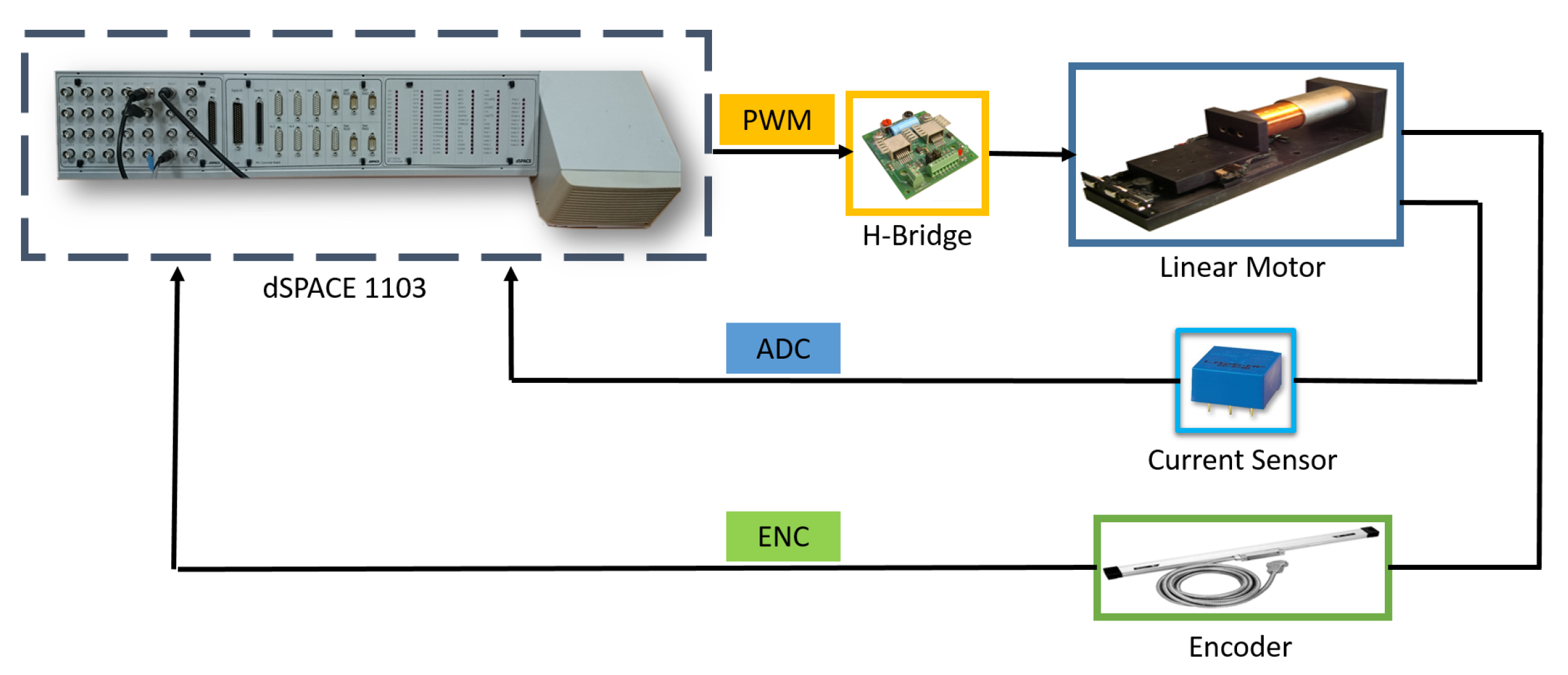
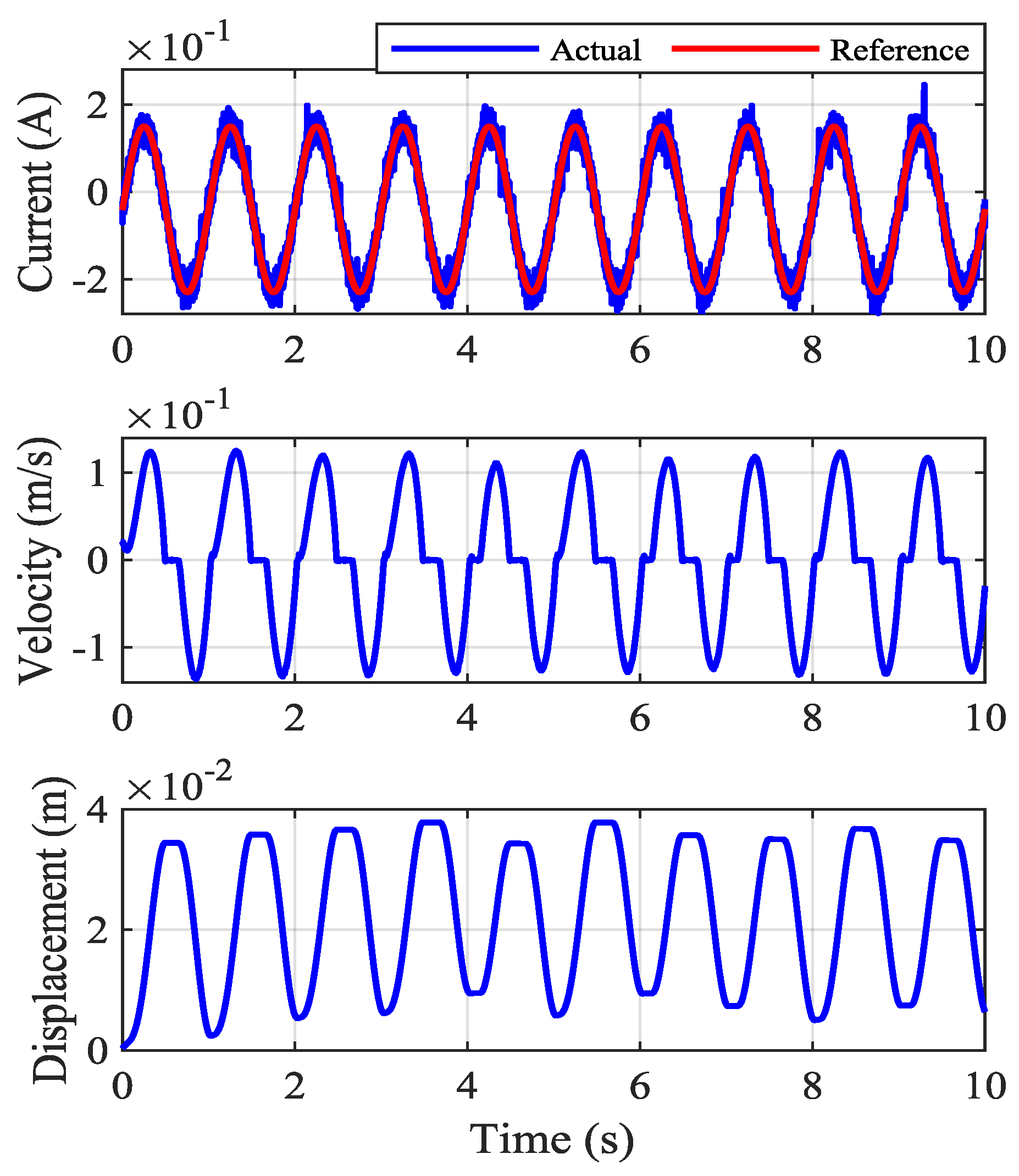
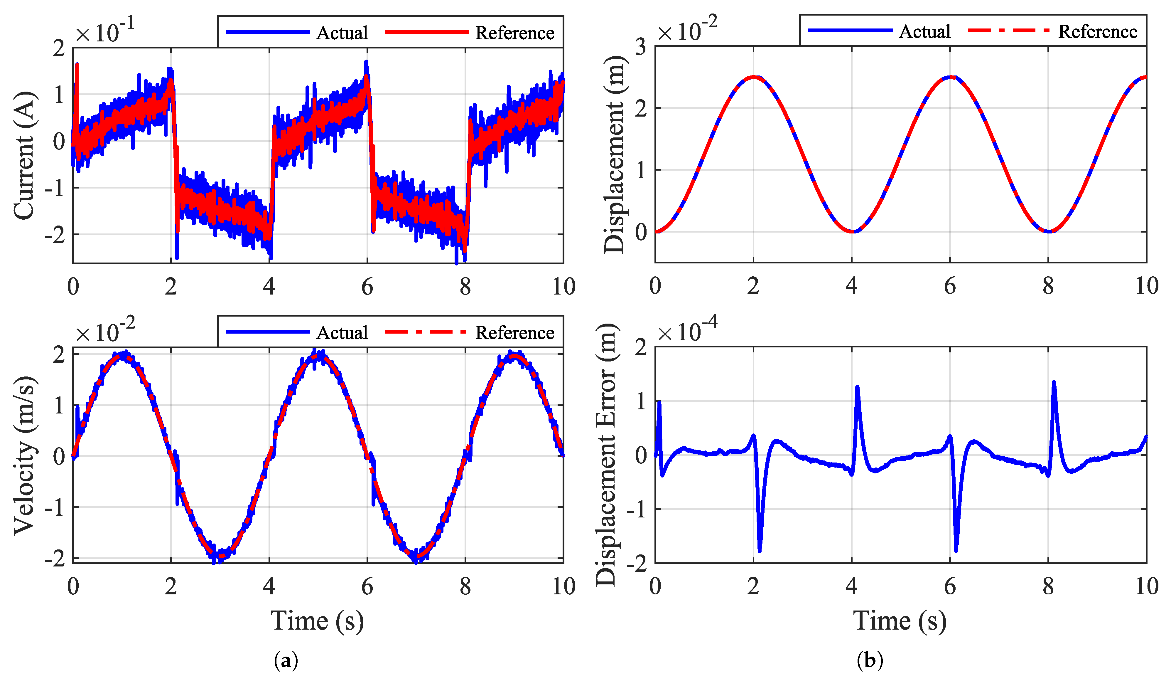
Section 5 discusses the experimental setup and results. Finally,
Section 6 concludes the paper with a summary of the conclusions.
3. Controller Design
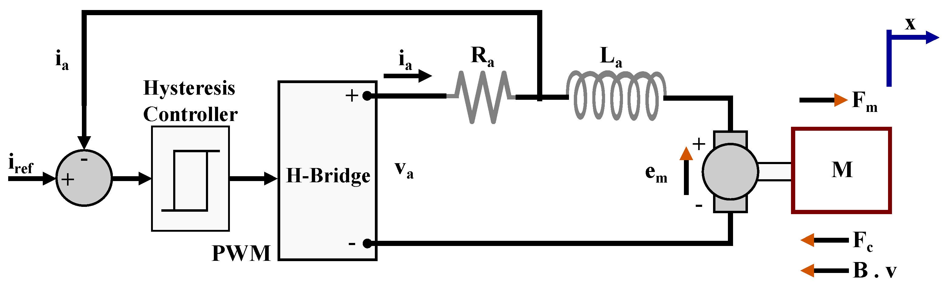
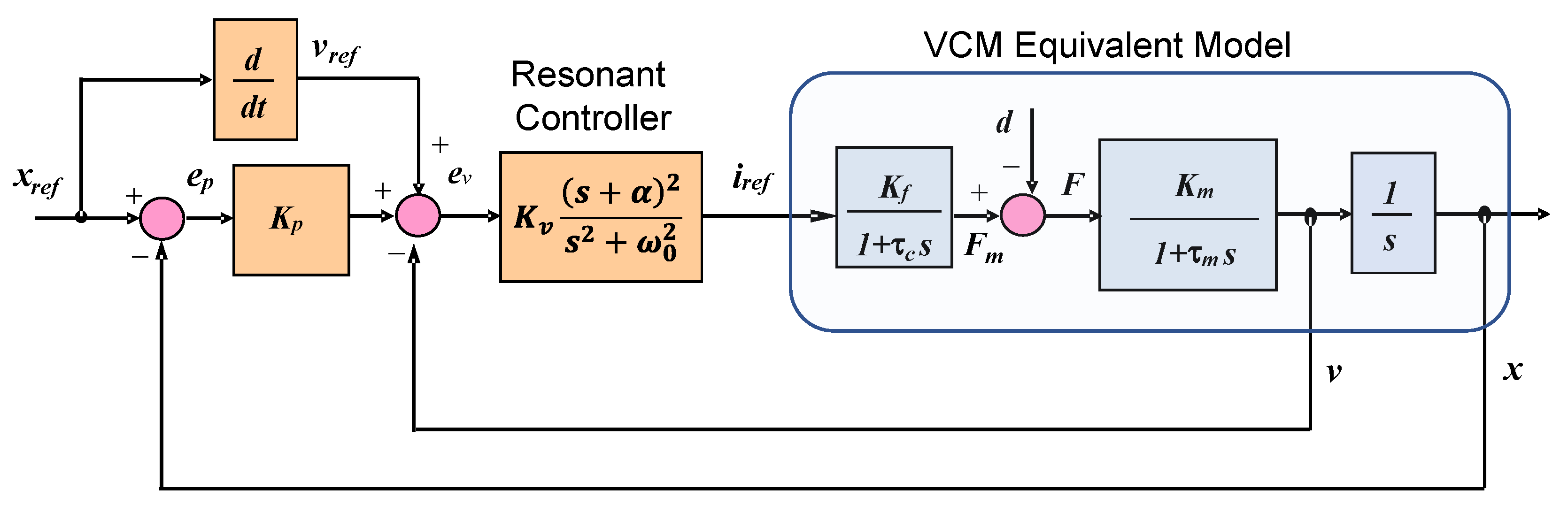
The proposed STRC controller is designed to track the reference position using a cascade control structure with an inner current/force control with hysteresis current control followed by a speed control loop with a resonant controller, and an outer position loop with a proportional and velocity-feedforward controller. The proposed control scheme is illustrated in
Figure 2. The linear motor drive system is represented by its equivalent block diagram with the internal current control loop. The main disturbance consists of Coulomb and sticktion frictions. Any additional load torque is represented as a disturbance to the linear system.
For the velocity control loop, we propose a new particular structure of a resonant controller. Its transfer function is given by:
where
and
are the controller parameters to be tuned and
is the reference signal frequency in (rad/s).
According to the internal model principle, the resonant control system will asymptotically track sinusoidal references and reject disturbances at the given frequency. The primary task of a resonant controller is achieved through the following control action:
Similar to the integral action in the case of a constant reference, this resonant control action is able to provide the required stability and zero steady-state tracking error. Using the same principle as in a PID control, added control actions can be incorporated to achieve suitable performance. Taking the derivative and integral of the main (resonant) control action yields:
The resonant controller given by (10) can be therefore written as a linear combination of the additional control actions:
Only two parameters need to be selected for the resonant controller, which simplifies the design procedure. The design procedure can be summarized as follows. and are selected such that fast transient response and stability are achieved. should be set to a value high enough to guarantee the stability of the internal velocity loop. The advantage of this resonant controller is that the stability margin is not compromised when is increased. The boundary condition on is defined by using Routh’s stability criterion and the root locus method.
Let
and assume the disturbance to be zero. Then, the internal velocity open-loop transfer function is given by:
The closed loop transfer function for the internal velocity loop is given by:
where
The outer position loop includes a proportional controller and a velocity-feedforward controller. The position controller is given by:
The open loop transfer function for the whole system is given by:
The closed loop transfer function for the system is given by:
The overall control scheme parameterization makes the STRC controller a function of three parameters, namely the position loop-gain , the resonant controller gain , and the zero . The flexible range of these variables greatly simplifies the tuning process as described in the following section.
3.1. Velocity Controller Design
Velocity controller gains are designed by deriving the upper and lower bounds using the stability analysis of the velocity control with the Routh–Hurwitz criteria [
41]. Given the denominator of the closed loop transfer function in Equation (
16), the Routh table is derived as shown in
Table 1.
To simplify the calculations, let:
Then, the terms
,
,
, and
in
Table 1 can be found to be:
For the system to be stable, the terms
,
, and
must be greater than zero. For condition
,
can be found as:
A conservative boundary condition for
can be used which allows for
to be chosen independently of
as follows:
Rearranging the condition,
leads to the boundary conditions:
and
A conservative condition for
can be used which allows for
to be chosen independently of
as follows:
On the other hand, the condition is always satisfied when .
The resonant controller-tuning procedure can be summarized as follows:
- •
The variable
is selected to satisfy the condition given in (
29).
- •
The gain
is selected to satisfy the condition given in (
32).
- •
The above two conditions can be achieved without the exact knowledge of the mechanical system parameters , , , and . Only approximate values of these parameters are needed to select the appropriate controller variables and assure system stability.
- •
The current control loop time constant is usually very small compared to the mechanical time constant . Therefore, . This gives more flexibility in the selection on the variable .
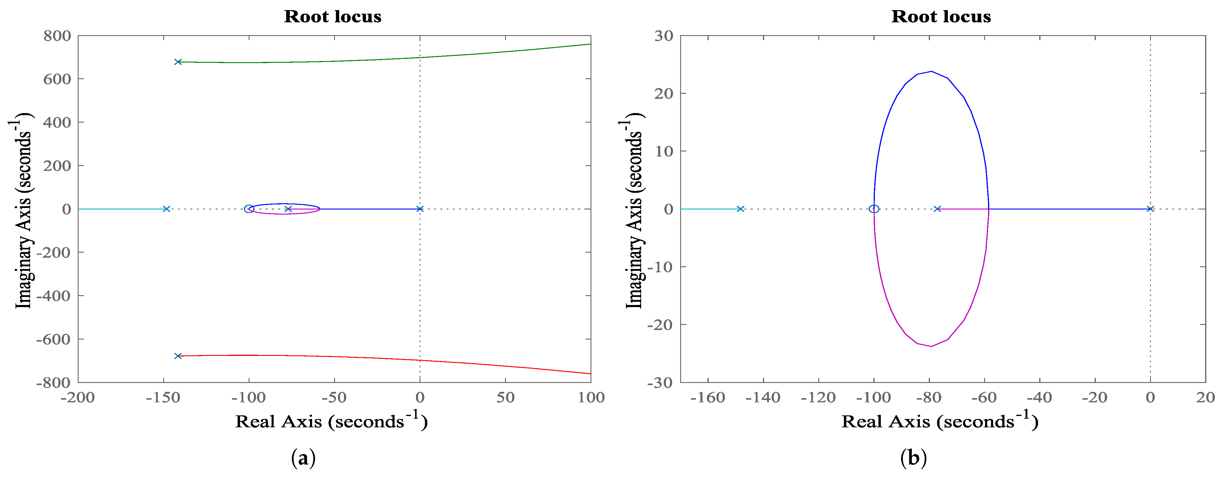
Figure 3 shows the root locus plot for the velocity loop as a function of the gain
for
. It can be shown that, for different values of
, the system is always stable if
is bigger than the lower bound set by Equation (
32). This lower bound corresponds to the crossing of the imaginary axis on the root locus as
is increased. Therefore, as the gain
is increased, a higher stability margin is achieved.
3.2. Position Controller Design
The position controller gain is designed by deriving the upper bound using the closed-loop transfer function given by (
20) along with the Routh–Hurwitz stability criteria. The Routh table is shown in
Table 2.
The terms
,
,
,
,
, and
in
Table 2 can be found to be:
For the system to be stable, the gain
should satisfy the following four conditions. The variables
and
are assumed to be given and have been selected based on the velocity-loop stability criteria.
The
condition is:
where
Equation (
44) can be solved by calculating the roots
and
of the equation and setting
to be between the roots
.
The
condition results in a third order inequality for the gain
:
where
and
Equation (
48) can be solved graphically using the Matlab Symbolic Toolbox to find the upper bound on
for given values of
,
, and
. The Matlab Symbolic Toolbox utilized in our work was version 2021b provided in the MATLAB software suite developed by
© MathWorks, Inc. (Natick, MA, USA). The Matlab Symbolic Toolbox is a tool in MATLAB for symbolic math computations, including solving mathematical equations and performing calculus operations.
Figure 4 shows the root locus plot for the outer position loop as a function of the gain
for
,
, and
.
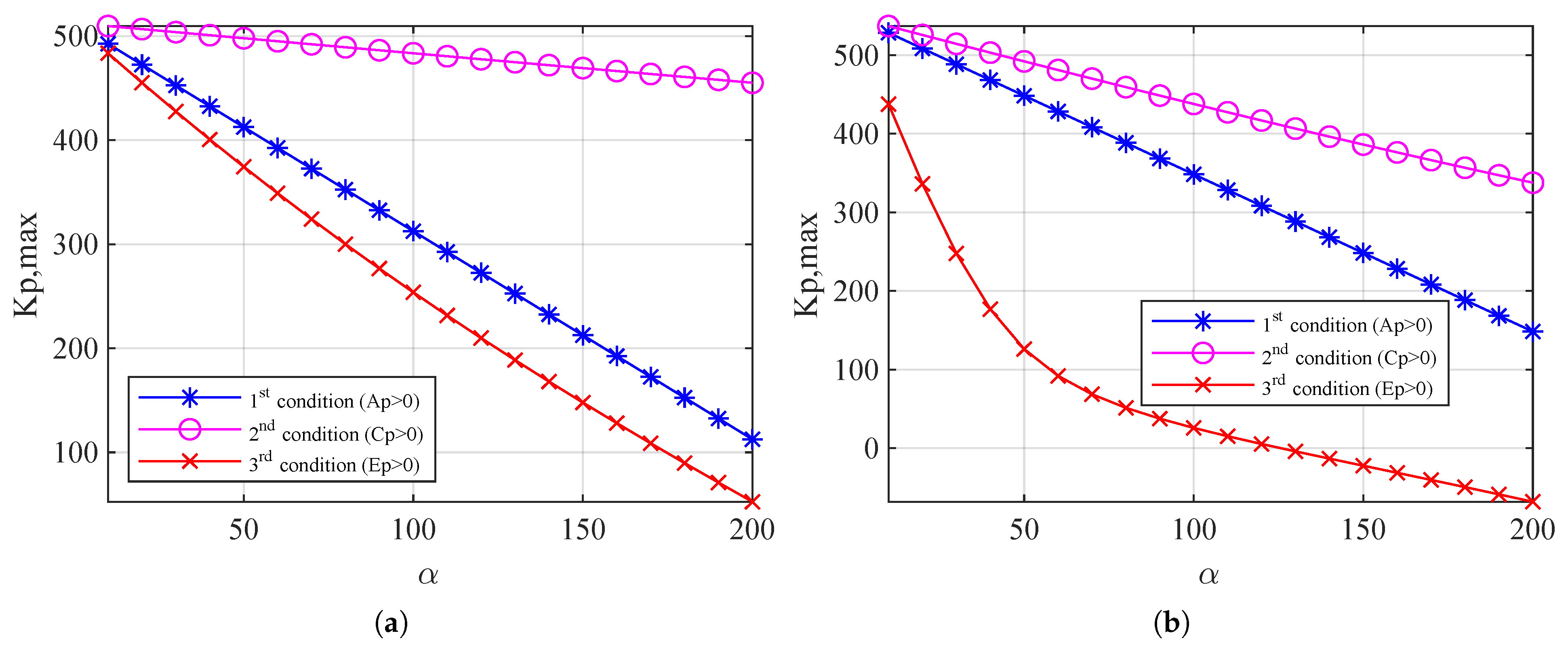
Figure 5 shows the upper boundary curves obtained from the conditions in (
39). It can be observed that boundary condition
is the dominant curve to limit the value of
. For a large value of the gain
, the curves for
and
get close to each other. It was also observed that the variable
has little effect on the second and third boundary conditions. Since the analytical expression of condition 1
is relatively simple, it can be used to find the upper boundary condition for
when
is relatively large.
4. Active Disturbance Rejection Controller
The active disturbance rejection controller (ADRC) is one of the highly effective controllers that have been shown to be superior to classical PID controllers. The ADRC was first proposed by Prof. Han Jing-Qing in 1995, and it has been used in various applications in much of the relevant literature [
23,
42].
The ADRC is a nonlinear controller with an error-driven scheme that can effectively control a dynamic system without requiring an accurate model [
42].
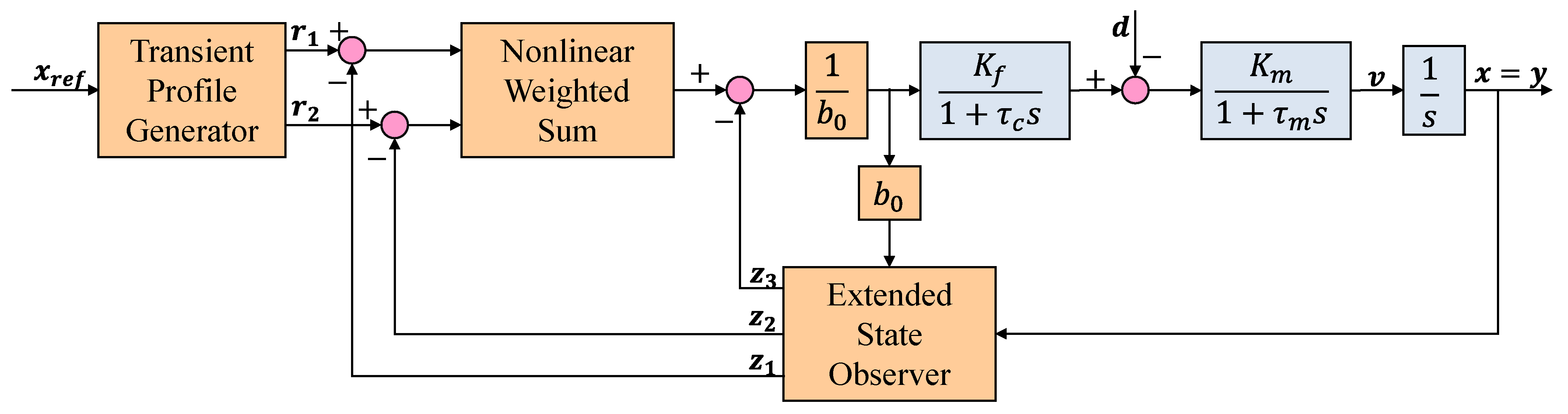
Figure 6 shows the configuration of the controller, consisting of three main components: a tracking profile generator (TPG), a nonlinear weighted sum (NWS), and an extended state observer (ESO).
In reference tracking systems, it is desired to design reference signal
in a physically feasible way to minimize tracking and initial errors. The TPG, introduced by Han, is a reference generator used in ADRC to smooth sudden changes in the reference signal. It helps to track the output of the TPG during sudden overshoot, reducing unexpected overshoot and rapidity of the PID controller while preserving the system response speed [
42]. The TPG can be designed in the discrete-time domain as follows:
where
is the control target,
is the derivative of the desired trajectory at
t, and
h is the sampling time. Han’s function,
, represents Han’s function with parameters
, the tracking speed factor, and
, the tracking filtering factor.
controls the speed of transition and
affects the smoothness of the output response [
42,
43]. The Han’s function
is defined as follows [
42,
43]:
The parameters
and
are adjusted individually to match the desired tracking speed and smoothness of the system’s output response, but there is no constructive technique for tuning them, as per [
43]. The NWS uses a nonlinear function that relies on error signals to produce the control signal. It calculates state variable errors by taking the difference between the TPG output and ESO state variables. Then, the control signal
is derived, as per [
43].
where
and
,
,
and
are controller gains, and
,
,
and
are the parameters of the function
. Substituting (
59) in (
64), if the ESO is very accurate, the result of
can be negligible. Therefore, (
59) can be written as,
The controller’s tuning is simplified by setting
and
, where
is the closed-loop control bandwidth [
24,
25,
43]. The larger
is, the faster the response. Both
and
are limited by hardware constraints, and
is commonly set to
.
The ESO uses dynamic functions to estimate unmeasurable variables, such as errors and disturbances. It outputs 3 signals:
approximates
,
approximates
, and
approximates disturbances. The control signal is adjusted based on the ESO estimates’ accuracy. Equation (
61) defines the observer design, and observer gains are tuned by
in Equation (
63).
where
,
, and
are observer gains, and
,
,
, and
are parameters for the function
in Equation (
62):
where
is specified in the range
and
is a multiple of the sampling time
h.
A greater value for means the observer runs faster.
As seen in
Figure 6, the ESO takes system output
and control signal
as inputs. It generates 3 signals:
approximates
,
approximates
, and
approximates disturbances. The ADRC adjusts control based on the ESO’s accuracy in estimating uncertainties, including model errors [
24,
42,
43].
Consider a dynamic system represented by the following equation [
23,
42,
43]:
where
is the system’s output,
is the control signal,
is an external disturbance, and
is an approximate estimate of the control signal gain.
is the generalized disturbance that is estimated in real time and compensated by the control signal,
[
44].
Let
,
=
and
=
. Assuming the unknown function
is differentiable, then
, and the system can be expressed in the state-space model as follows:
with the system state
.
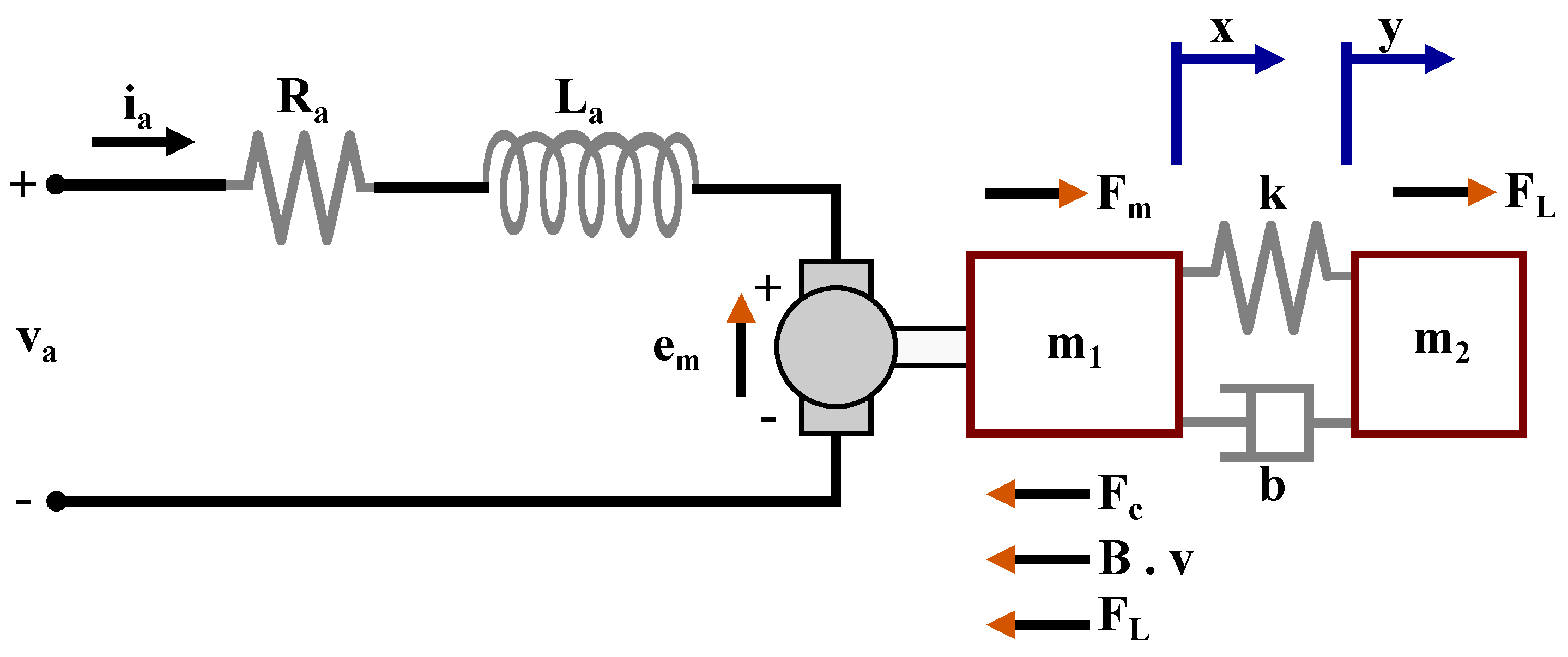
For the voice-coil motor, the mechanical system equations with current control reduce to only Equations (
3)–(
5), which can be expressed as:
If the Coulomb friction is considered as a disturbance
d, Equation (
66) can be written as:
Both viscous and Coulomb frictions can be combined as the generalized disturbance
. Equation (
66) can now be written as:
where
If the current control loop is assumed to be very fast, then:


