Abstract
This study aims to improve the vehicle vertical dynamics performance in the sprung and unsprung state for in-wheel-motor-driven electric vehicles (IWMD EVs) while considering the unbalanced electric magnetic force effects. An integrated vibration elimination system (IVES) is developed, containing a dynamic vibration-absorbing structure between the IWM and the suspension. It also includes an active suspension system based on a delay-dependent controller. Further, a novel frequency-compatible tire (FCT) model is constructed to improve IVES accuracy. The mechanical-electrical-magnetic coupling effects of IWMD EVs are theoretically analyzed. A virtual prototype for the IVES is created by combining the CATIA, ADAMS, and MatLab/Simulink, resulting in a high-fidelity multi-body model, validating the IVES accuracy and practicability. Simulations for the IVES considered three different suspension structure types and time delay considerations were performed. Analyses in frequency and time domains for the simulation results have shown that the root mean square of sprung mass acceleration and the eccentricity are significantly reduced via the IVES, indicating an improvement in ride comfort and IWM vibration suppression.
1. Introduction
Automotive electrification is rapidly expanding worldwide to tackle the challenges such as greenhouse gas emissions and fossil oil depletion. In-wheel-motor-drive electric vehicles (IWMD EVs), in which the drive motor is integrated directly into the wheel, have several benefits, including compactness, controllability, and efficiency. Recently, IWMD EVs started to attract researchers, and are an important research direction for future electric vehicles [1,2]. However, the use of wheel motors increases the unsprung mass, negatively affecting the vehicle dynamic performance, including ride comfort and road holding performance [3,4]. On the other hand, increasing expectations for improved noise-, vibration-, and harshness- (NVH) performance make it more important to deeply investigate correlated characteristics [5,6]. Additionally, IWM vibration might cause motor bearing wear and magnet gap eccentricity [7]. Further, eccentricity can cause an unbalanced electric magnetic force (UEMF) which further distorts the air gap distribution, exacerbating the in-wheel-motor (IWM) vibration, creating a vicious cycle [8]. This is known as a typical mechanical-electrical-magnetic coupling system where UEMF has a key role [9,10].
Numerous studies were carried out to mitigate the adverse coupling effect on vehicle dynamics, and can generally be grouped into two categories. The first category includes designing the IWM as a dynamic vibration absorbing structure (DVAS), where the IWM is isolated from the axle by spring and damper elements [11]. The DVAS absorbs the vibration energy transmitted to the IWM by damper element [12]. Further, DVAS is generally divided into “chassis DVAS” and “tire DVAS“, which flexibly connects the IWM to the sprung and unsprung masses, respectively [11]. Previous studies have shown that DVAS can partially suppress the IWM vibrations if the parameters of the additional spring dampers are properly selected [13,14]. Furthermore, an active DVAS control method is proposed in [15] through the installation of a controllable linear motor between the IWM stator and the wheel axle, effectively reducing the wheel vibration. Most existing DVAS installed in the IWM are passive vibration absorbers with fixed parameters, which cannot be adjusted to complex and variable road excitations. On the other hand, the active DVAS can achieve better performance but is seldom applied due to its cost and space constraints. In addition, when improving IWM vibrations, DVAS has difficulty optimizing sprung mass vibrations in the 4–8 Hz frequency range of the passenger-sensitive [16].
The second category considers the IWM suspension as a complete system, which utilizes conventional active suspension system (ASS) control algorithms to reduce the negative impacts of the increase in unsprung mass. Examples of such algorithms are explicit model predictive control method [17], fuzzy logic control [18], ceiling damping control [19], optimal sliding mode [20], and control [21]. Active suspension systems inevitably have time delay, which is one of the most important factors affecting the stability of the system. Among the above control strategies, control is widely used since it provides increased system robustness for time delay, and time constant perturbation [22]. Sun et al. [23] designed an adaptive robust controller for electro-hydraulic actuator active suspension, robust to the uncertainty of actuator parameters and its nonlinearity. In [24], the robust controllers were designed for ER suspension systems with parameter uncertainties. The dynamic bandwidth of the current-variable damper under the fast and slow response action was determined. Li et al. [25] proposed using a robust control method to improve vehicle performance under load variations. The required vehicle suspension properties such as ride comfort, car handling, and suspension deflection are transformed into a continuous time system with input delay and sector bounded uncertainty. Shao et al. [26] studied the control design method for an ASS of IWMD EVs while considering the actuator failure, time delay, and disturbances. Jing et al. [27] designed an ASS controller for IWMD EVs, aiming to isolate forces transmitted to the motor bearings and improve ride comfort. However, the ASS is a complex system with multiple parameters, and the mechanical-electrical-magnetic coupling effects will further aggravate this condition. Moreover, due to the time delay and power limitation of the actuator, the adjustable frequency range of the ASS is concentrated in the low and mid frequencies [28].
The DVAS and ASS significantly reduce the vibration of unsprung and sprung vehicle masses, respectively. However, few studies combined the ASS control strategies and DVAS approaches to mitigate the mechanical-electrical-magnetic coupling effects. Liu et al. [29] proposed a two-stage optimal control method to improve vehicle dynamics performance through ASS and DVAS. A linear quadratic regulator controller based on the particle swarm optimization and finite frequency controller are designed for DVAS and ASS, respectively. However, the UEMF of IWM and the time delay of the ASS were not considered. Wang et al. [30] explored the control strategy for an ASS system in the IWMD EVs, which reduced the IWM vibration and improved the ride comfort. However, the IWM UEMF was not considered. Liu et al. [31] used the particle swarm optimization algorithm to optimize the DVAS parameters, while the alterable-domain-based fuzzy control method was used to control the DVAS actuator force. However, the proposed integration structure was limited by its complexity and was not effectively validated. Since DVAS and ASS have different roles in the IWMD EVs, their combination strategies should be studied to improve motor and suspension performances.
Generally, simplified tire models including only the spring characteristics are used in vehicle vertical control; however, the increase in unsprung mass and the high-frequency excitation generated by the motor directly affect tire working conditions [32]. In particular, the increase in the unsprung mass causes an increasingly non-linear relationship between the contact force and the road roughness [33]. Typical tire models include physical and empirical tire models. The brush and ring models are two main forms of physical models; the magic formula tire model is attributed as an empirical tire model. However, brush and magic formula tire models are used for modeling the tangential tire force characteristics, not applicable for calculating vertical tire force [34,35]. The most commonly used models in vertical tire dynamics calculation is ring model, which is typically represented by the rigid ring model (RRM) [36] and the flexible ring model (FRM) [37]. For the former, the residual stiffness is introduced between the contact patch and the rigid ring to represent the static tire stiffness in the vertical directions. However, the tire belt deformation was not considered and the applicable frequency range during the analysis is usually low [36]. Further, the FRM uses a large number of segments interconnected by springs and dampers. The FRM bandwidth is thus up to 150 Hz, corresponding to the first flexible belt bending modes; however, it could rarely respond to low-frequency characteristics [37]. As to the IWMD EVs, there are complex maneuvers including high-frequency (50–100 Hz [38]) vibration of the IWM system, as well as low frequency excitations (under 20 Hz) from the road unevenness. Both groups exert serious influences on the vertical dynamics of the vehicle. Consequently, to improve the accuracy and adaptability, it is necessary to integrate the RRM and FRM.
As described above, the combination of DVAS and ASS should be comprehensively investigated to improve the vehicle vertical performance; the UEMF created by mechanical-electrical-magnetic coupling effects should also be considered. Additionally, an accurate road-tire-IWM model is necessary to simulate the real external excitation of the IWM suspension system. Finally, the scientific contributions of this study are:
- A novel IVES was developed, containing a practical DVAS equipped between the IWM and the suspension, as well as a robust ASS based on the delay-dependent controller. The UEMF was considered in this system and the mechanical-electrical-magnetic coupling effects of IWMD EVs were observed.
- A frequency-compatible tire (FCT) model integrating the RRM and FRM was developed to ensure adaptability to different frequency ranges. It also improved the accuracy of vertical tire forces, which were further inputted as an external excitation to the IVES (instead of the road roughness), further improving the accuracy.
- A novel virtual prototype was designed, combining CATIA, ADAMS, and MATLAB/Simulink environment to establish a high-fidelity multi-body model for the IVES. Particularly, the IVES structure was developed, aiming to maximize its integration ability and minimize the impact on the original chassis structure.
The remainder of the paper is organized as follows: the IVES mathematical model combined with the UEMF model, vertical vibration model, and driving model were introduced in Section 2. The proposed delay-dependent controller was outlined in Section 3. In Section 4, performed simulations and validations were described for the IVES in a virtual prototype. Finally, study conclusions are given in Section 5.
2. The Mathematical Model of SIWMS
The IVES mathematical model was developed, containing the UEMF model in driving conditions, an FCT model, and a DVAS-ASS integrated model. The investigated UEMF and FCT model tire force are imported into the DVAS-ASS integrated model as internal and external excitation, respectively.
2.1. The UEMF Model in Driving Conditions
For a switched reluctance motor (SRM), the electromagnetic force can be decomposed into tangential and radial forces according to the electrical angle [39]. The material of stator and rotor is ferromagnetic, the radial force of electromagnetic force is much larger than the tangential force [40,41], and the eccentricity of the rotor and stator of IWM will cause a large deviation of radial force, which acts on the stator of the IWM to produce a violent vibration. From the above analysis, it is evident that the UEM is produced by the coupled action of electromagnetic and mechanical fields and represents the resultant global magnetic force acting on the rotor and stator due to an asymmetric magnetic field distribution in the air gap, The UEMF generation process is shown in Figure 1. In the figure, is the tangential force, is the radial force, is the electromagnetic force.
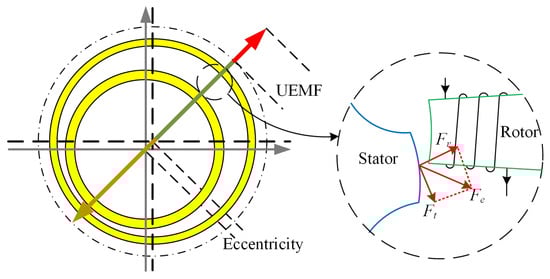
Figure 1.
UEMF generated in a SRM.
In this paper, a 5-kW exterior rotor switched reluctance motor (SRM) prototype with 8/6-four phases was used [42]. The magnetic co-energy W (i, θ) is determined according to the current i and the phase inductance L(θ, i), where is the rotor angle. The first three terms of L(θ, i) Fourier expansion are given by:
where L, L, and L are calculated as:
where L, L, and L are inductances at fully-aligned (θ = 30), unaligned (θ = 0), and intermediate positions, respectively. These parameters can be fitted with polynomials based on either the finite element analysis or the experiment. Considering the relationship between the flux and the inductance, the k-th phase flux linkage can be derived as:
where c = a/n and d = b/n. According to Faraday’s law, the phase voltage is:
where is the angular rotor velocity. The phase current can be written as:
For constant phase current i, relationships between the magnetic co-energy W (i, θ), torque T, and radial force F are defined as:
where l is the air gap between the rotor and the stator. The phase torque is found using:
where both e and f are intermediate functions. The former, e, can be calculated as = (1/2) , = 0, and = (1/2) ( − ). The latter, f, is given by = − , = 0, and = (1/2) (2 − − ).
Based on the phase torque T, the radial force of the k-th phase can be calculated as [11]:
where is the overlap between the rotor and the stator. The presence of non-zero would result in the UEMF. There are many possible causes for eccentricity, including poor manufacturing accuracy and dynamics coupling effects [43]. The eccentricity can be decomposed into x- and z-axes, and the resulting components are expressed as and . In this study, the dynamic eccentricity in the z direction due to the road excitation of the vehicle while driving is mainly investigated. the UEMF decomposition in the vertical direction is shown in Figure 2.
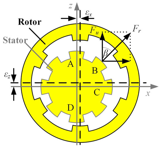
Figure 2.
The vertical UEMF induced by eccentricity.
Based on the UEMF definition and the mixed-eccentricity, the vertical UEMF F is [11]:
where is the phase structure angle () and the nominal air gap is 0.8 mm.
The strategy uses a current chopping controller to avoid the stator winding resistance stemming from consuming the electrical energy; the preset current limit is 23 A. Due to the configuration of the adopted SRM model, the given turn-on angle ranges between 0 and 12, while the turn-off angle range is between 22 and 30. In this paper, the main role of SRM is to provide driving torque. The driving torque mean value and standard deviation were used as indexes, and the results are shown in Figure 3a,b. Based on the results, angle and values are selected as 4 and 28, respectively. Using these control parameters, the single-phase UEMF of SRM in both vertical and longitudinal directions are characterized by different and values. The results are shown in Figure 3c.
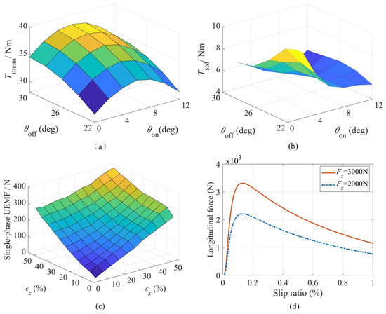
Figure 3.
The IWM characteristics: (a) versus turning angle; (b) versus turning angle; (c) single-phase UEMF of SRM; (d) the magic formula.
To simplify the calculation, it was assumed that the motor stator eccentricity direction of is vertical. The eccentricity can directly affect the UEMF, which is represented in form of the electromagnetic coupling of the system. The wheel rotation equilibrium equation is as follows:
where is the rotational inertia of the total wheel, is the effective rolling radius, M is the rolling resistance moment generated by the tire, F is the reaction force between the tire and the road obtained by the magic formula [35] (see Figure 3d), T is the motor drive torque, F is the vertical dynamic load, is rolling resistance coefficient, is the quarter total vehicle mass, and is vertical tire force discussed in Section 2.2.
2.2. The FCT Model
Next, the FCT model, which applies both the RRM and FRM, was integrated to capture the transient tire-road contact patch and tire belt deformation.
The road roughness z is commonly described via power spectral density in the vertical direction. The Harmonic superposition algorithm was used to generate time-domain road profiles [44,45]:
where is the K-th middle frequency and is the power spectral density at . Further, is an identifiably distributed phase with the range of (). The upper and lower time-domain frequency boundaries are denoted as f and f. Finally, according to the ISO-8608 [46], ISO-A, ISO-B, and ISO-C road displacement spectrum as shown in Figure 4. In this paper, the ISO-B was adopted as the actual road excitation.
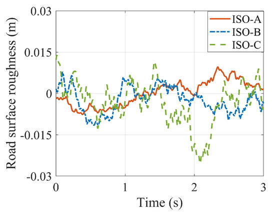
Figure 4.
The road displacement spectrums.
When a tire is loaded on the road, a large deformation having a limited contact length occurs near the contact patch, which could be equated to a contact point [47]. Moreover, the vertical residual stiffness of RRM was introduced to determine the overall vertical tire stiffness [36]. The residual stiffness k is equal to:
where z is the vertical tire displacement, is the angular tire velocity, is the vertical stiffness correlation coefficient of the tire.
The vertical contact point force F is directly related to the k. The tire deformation within the contact patch can be equated to the contact point deformation using a deformation stiffness of k, as shown in Figure 5. After neglecting the higher-order terms, a third-order polynomial was used to describe the vertical force due to the residual tire deflection [36]:
where are polynomial coefficients expressed as:
where q, q, and are vertical stiffness correlation coefficients of tire and k is its sidewall stiffness.
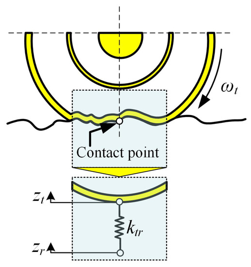
Figure 5.
The equivalent process for deformation.
The RRM only considers the contact point deformation; the tire force generated by the tire belt in the contact patch is not calculated—the FRM was used to calculate it. The model includes a finite number of independent radial springs and damping elements evenly distributed in the lower semicircle, as shown in Figure 6 [48]. The total number of the discrete radial elements is denoted as N [49].
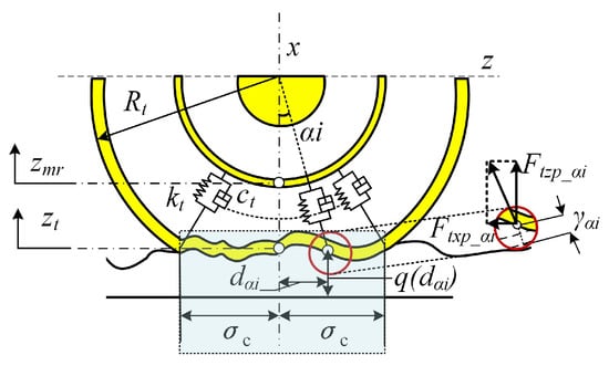
Figure 6.
The illustrative representation of the FRM.
In Figure 6, is equal to the half of the contact patch, is the vertical coordinate of the rotor center, z is the vertical contact point displacement, denotes the tire damping, and αi represents the angle between the arbitrarily chosen element and the vertical, ranging from 1 to N.
For the positive x-axis, the subscript i indicates the element sequence number ranging from −arcsin(/R) to +arcsin(/R). Further, , , and q(d)arethe radial deformation, driving distance, andthe element road elevation, respectively. As a result of tire deformation, the vertical component F of the radial spring and damping element forces are:
The deformation and deformation rate of a certain radial element can be approximately calculated using:
where x is the longitudinal displacement of the tire. The vertical tire force component F caused by tire deformation at the rotor center can be obtained by summing up the force components of each spring and damping element:
In general, the vertical tire force calculated through the FTC model under road roughness excitation is:
Finally, is further employed as an external excitation to the IVES (instead of the road roughness).
2.3. DVAS-ASS Integrated Model
The quarter models of three types of suspension structures were created in this section. Since the sprung mass distribution coefficients in most modern vehicles are designed to be close to 1. Furthermore, in the suspension structure of the IWMD EVs configured with ASS, the four wheels are independent of each other in vertical motion. Therefore, the quarter model is representative when studying the vertical motion of the vehicle [50]. The sprung and unsprung mass are included, as well as the suspension and tires.
Figure 7a shows a passive-suspension system in which the IWM stator and rotor are rigidly connected to the axle and hub, respectively. Therefore, the IWM becomes the unsprung vehicle mass; is the quarter of the vehicle sprung mass, m is the rotor mass, m is the sum of the stator, axle, and tire mass, k is the motor bearing stiffness, k is the suspension stiffness, c is the suspension damping, F is the UEMF, and represents displacement (where index “” stands for r, , , s, or ). In a passive-suspension system, the IWM is directly impacted due to rigid joints, which deteriorates its reliability and service life. On the other hand, the IWM equipped with the DVAS is a good solution to suppress the vibration problem, as shown in Figure 7b. Variable m represents the sum of the axle and tire masses, while k and c are the stiffness and damping of the absorber, respectively.
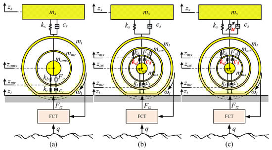
Figure 7.
Quarter vehicle models equipped with the IWM: (a) passive suspension, (b) DVAS, (c) ASS and DVAS.
The DVAS mechanism is, in theory, similar to that found in passive suspensions. To simultaneously improve the vibration performance of both the IWM and the sprung mass, a suspension combining the ASS and the DVAS was used as the object; its configuration is shown in Figure 7c, u is the active-controlled force of the ASS.
By combining the models shown above, the overall logical diagram of the proposed mechanical-electrical-magnetic coupling model of the IVES was obtained and is shown in Figure 8. For a given road profile (ISO-B was used in this paper), the vehicle speed determines the vertical road excitation z. The road excitation causes wheel vibration, which results in the eccentricity between the rotor and stator. The coupling effect between and the UEMF model produces F. For the driving model, z, z, and wheel speed in unison determine the and . Further, F and the slip ratio between vehicle and wheel determine the magnitude of F, while the current chopping controller adjusts the voltage (on/off) of the IWM. The control signal of the IWM is adjusted according to the difference between the vehicle and the set speed, which is the input to the vibration model and w, closing the loop.
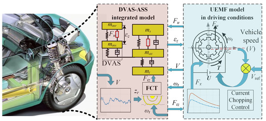
Figure 8.
The Multi-field coupling model of IVES.
3. The IVES Optimization Control
In this section, the UEMF effects on the suspension system were analyzed, and the outcomes were improved by developing a delay-dependent controller for the ASS.
3.1. The UEMF Influence on the Dynamic Performances of the Vehicle
Based on the above-mentioned mathematical models, a simulation platform for the vehicle multi-field coupling dynamics can be developed using MatLab/Simulink. Test vehicle specifications are listed in Table 1. The DVAS “tire” type [11] and air spring active suspension [51] were selected as actuators in this paper. The tire used in this paper is a passenger car summer tire designated as 205/55R16 [52].

Table 1.
Test vehicle specifications.
The dynamic coupling relationships were investigated assuming the ISO-B road at a speed of 40 m/s. The drive lasted for 3 s and the Fast Fourier Transform (FFT) was used to derive spectral features. For observation, 1–2 s data points were selected for further statistical analysis. The responses of sprung mass acceleration (SMA) and eccentricity (ECC) with and without the UEMF under the pavement excitation are shown in Figure 9.
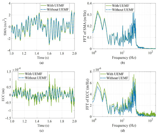
Figure 9.
Coupling effects between the SMA, the ECC, and the UEMF: (a) the SMA time response; (b) the SMA frequency response; (c) the ECC time response; (d) the ECC frequency response.
The time-response results have shown that the SMA and ECC are larger when considering the UEMF effects. The same trend can be deduced from the frequency response—the effect of UEMF on the ECC at high frequencies is particularly pronounced.
The eccentricity between the stator and rotor was further exacerbated by the UEMF generated by the multi-field coupling effect. Such eccentricity, in turn, furthers the UEMF, which is complementary to it. This vicious cycle exacerbates motor vibration, shortening the IWM service life and reducing vehicle comfort. Therefore, it is worthwhile to investigate the issue of how to restrict the multi-field coupling effects.
3.2. Active Suspension Control
An control scheme with strong robustness was used to design the active suspension controllers. The controllers were needed to ensure excellent control effect of the suspension system when given complicated electromagnetic force excitation and un-modeled dynamic perturbation. According to Equation (21), the following set of state variables was selected:
The dynamic equations of the ASS with the DVAS system can be written using the following state-space form:
where:
Generally, the suspension performance is evaluated based on key factors such as ride comfort, suspension working space, and road-holding ability. Additionally, as for the IWMD EVs, the IWM UEMF is an essential performance factor. Thus, four system responses are investigated: SMA: , rattle space (RS): − , tire deformation (TD): ( − ), and ECC: ( − ). Among these, the first three are used for evaluating the suspension performance, whereas the last one reflects the IWM vibration level.
Focusing on ride comfort improvement and the IWM working environment, the SMA and eccentricity should be minimized, while the other two factors are strict constraints that must be satisfied. Therefore, minimizing the disturbance transfer function norm (F and F) to the control output ( and ( − )) is our main goal. The constraints as follows:
where z and z are the maximum suspension and tire deflection, respectively. u is the maximum possible actuator output force.
Based on the above-presented conditions, the performance control output and constrained control output are defined next:
The state-space equations of the ASS and DVAS for the IWMD EVs can be described using:
where:
The ASS inevitably has operating time delays, with the majority being the response time delay of the actuator. Hence, time delay should not be neglected when designing the active suspension system.
Assuming that the time-varying delay (t) in a closed-loop controlled suspension system satisfies the condition:
where represents the upper bound of the delay time. Considering the delay time, the output feedback controller can be described as:
where K is the output controller gain. Next, the ASS that considers the time delay in the control system can be expressed via:
In this paper, the aim is to design a state feedback controller that will meet the following conditions:
Considering the time delay, the controller was designed through the following steps:
Given positive scalars , , and , for any time delay t satisfying , the system shown in Equation (26) with the controller from Equation (29) is asymptotically stable with w(t) = 0. In that case, it also satisfies the performance described in Equations (25) and (26) for , given that symmetric matrices P > 0, Q > 0, and R > 0 exist, and a general matrix K satisfying the following linear matrix equations (LMIs) is:
where:
For comparison, the controller without considering time delay is obtained as follows:
For a given scalar , if and a positive definite symmetric matrix X exists, making the following inequalities feasible under LMIs:
The state feedback gain K can be given by K = WX
Proof.
Lemma 1 [53]: For any matrix X > 0, matrices (or scalars) M and N with compatible dimensions, the following inequality holds:
Since , by adding it to Equation (30):
Selecting the Lyapunov function shown below to analyze the system stability we obtain:
where:
with P, Q, and R being symmetric positive definite matrices. The derivative of is shown next:
Using Lemma 1, that gets:
Similarly, derivatives of and are expressed as:
Further, the derivative is shown as follows:
Defining , thus
where:
The system performance can be described as:
By adding to Equation (43), it is possible to obtain:
where:
For any positive scalar , the following expression is true:
By replacing the item in with , we get . Moreover, it is true that , where:
If the matrix inequality , that .
From inequality Equation (45), it can be derived that . Integrating both sides of the inequality above from zero to any , the following is obtained:
Considering the existence of , the above inequality can be further rewritten:
Definition , where w is upper perturbation energy bound, can be introduced with a value equal to , Therefore, it can be introduced under and within a given perturbation suppression regime . In combination with , synthetically, the following inequalities hold:
This causes matrix inequality . Using the Schur complementary theorem [54], the equation is converted into:
For a case without a time delay controller, the proof can be found in [55].
The proof is completed. □
4. Simulation and Analyses
In this section, the influence of the ASS and DVAS on the IWMD EVs performance, as well as the effectiveness of the delay-dependent active suspension controller is illustrated.
4.1. Performance Comparison of Different Structures
Four system responses, the SMA, the RS, the TD, and the ECC were investigated in Section 3. For the maximum time-delay = 40 ms, Equations (31) and (32) are LMIs of variables P, Q, and R. Thus, the program can be solved via the solver-mincx within the LMI toolbox. Through LMI algorithms, the control gain matrix K of the ASS controller (considering the time delay) is obtained with the minimum guaranteed closed-loop performance index = 8.82. Such output implies that for any time-delay satisfying , the controller can stabilize the system with the performance.
Similarly, a conventional controller without considering the control time delay can be derived. The gain matrix K of the Controller with the minimum guaranteed closed-loop performance index = 6.28 is obtained as:
After the method proposed in this study to solve the multi-objective control problem of the ASS, its effectiveness is illustrated through four different cases:
- Case 1—equipped with the IWM and passive suspension;
- Case 2—equipped with the DVAS in IWM and passive suspension;
- Case 3—equipped with the DVAS in IWM and the ASS using the control gain matrix K;
- Case 4—equipped with the DVAS in IWM and the ASS using the control gain matrix K.
Figure 10 shows the controller forces applied on the ASS in cases 3 and 4. Both controller forces are less than umax. Further, the controller force in Case 4 is smaller than that in Case 3.
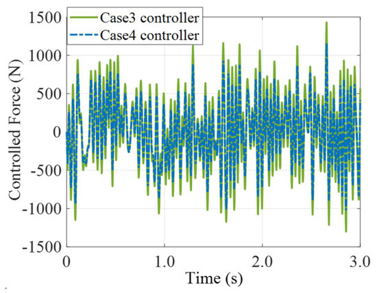
Figure 10.
Controller forces in Case 3 and Case 4.
The response comparisons of the two-output time and frequency domains of the SMA and ECC are depicted in Figure 11.
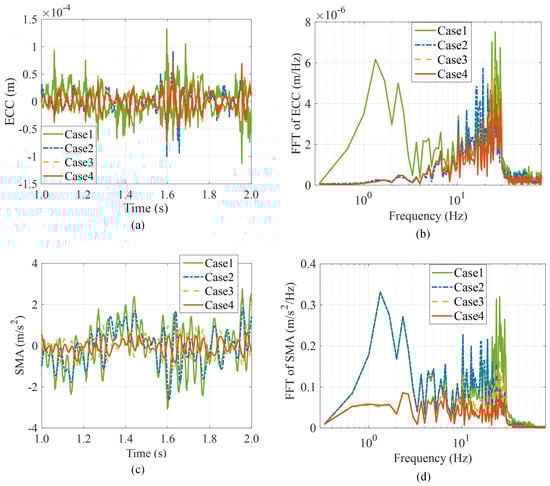
Figure 11.
Responses of four cases under the road excitation: (a) SMA time response; (b) SMA frequency response; (c) ECC time response; (d) ECC frequency response.
The detailed simulation results are available in Figure 11. The responses of the SMA in time and frequency domains are shown in Figure 11a,b, respectively. As shown in Figure 11a, the SMA is significantly smaller in cases 3 and 4 compared to cases 1 and 2, mostly due to the introduction of the ASS. Figure 11b shows that Case 2 can reduce the amplitude of high-frequency compared to Case 1; however, there is no optimization effect at the human-sensitive frequency of 4–8 Hz. Cases 3 and 4 can significantly reduce the amplitude in both high and low frequencies (especially compared to Case 1), especially in the 4–8 Hz range.
The ECC responses in time and frequency domains are shown in Figure 11c,d, respectively. As shown in Figure 11c, in contrast with the SMA optimization effect, all three cases had reduced amplitude in the wide frequency domain concerning Case 1. The proposed control methods of the active suspension are effective for the IWM vibration. The SMA is smaller in cases 3 and 4 compared to in Case 2 in the frequencies between 3 Hz and 12 Hz, indicating that the proposed control method for the ASS can further reduce the impulse force acting on the IWM.
Simulation results for all four cases are provided in Table 2.
Table 2.
Root Mean Square (RMS) optimization results.
As can be seen from Table 2, both the DVAS and the ASS can reduce the four-parameter indices, while having different roles in improving comfort and handling. The DVAS has an important role in reducing eccentricity, while the ASS has a decisive effect on spring acceleration. For the RS and TD, the optimization effect is not significant compared to the conventional suspension since they are not optimized in a targeted way. At the same time, the H-infinity algorithm, which considers the time delay, displayed a performance improvement compared to the algorithm not considering it.
Table 3 compares control methods in terms of simulation results considering the presence of time delay in the active suspension actuator. It also indicates that, with the increase in time delay, both Case 3 evaluation indexes deteriorated to different degrees; the SMA deterioration is obvious. In contrast, Case 4 adapted easier and the degree of deterioration was not significant—it was within acceptable limits.
Table 3.
The RMS optimization results for both cases.
4.2. Virtual Prototype Validation for the IVES
A virtual prototype (VP) enabled the proof testing before assembling the hardware, reducing both the manufacturing cost and time. The design possibilities of the IVES can be explored through the VP, and the study of tradeoffs between IVES component sizes becomes feasible. In this part, an VP, combining CATIA, ADAMS, and MatLab/Simulink environment was constructed to establish a high-fidelity multi-body model for the IVES.
The build process used to create the VP model is shown in Figure 12. Firstly, a complete vehicle model was parametrically modeled in CATIA, using the vehicle model parameters obtained from an actual IWMD EV. Then, the IVES model was imported into the ADAMS and the constraints of each component were established. The collision model of each component was established, the corresponding material was defined, and the loads and drives were added. Finally, the driving torque and controller force of the ASS was taken from the IWM system modules and ASS controller modules available in MATLAB/Simulink, respectively. For the UEMF, the vertical force F was applied to the IWM rotor and stator surfaces.
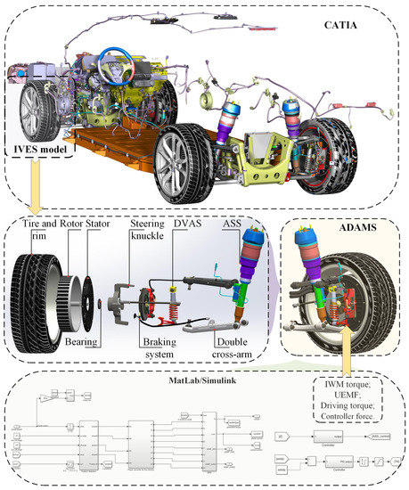
Figure 12.
The VP building process.
As shown in Figure 12, using a connector, the DVAS is linked to the steering knuckle at the upper end and the IWM stator at the lower end. Since the axle is kept in steering synchronization with the IWM, there is only relative vertical motion between the two. The lower ASS end is fixed to the lower cross arm of the double cross arm; the control force is output through the ASS sensor. The proposed IVES structure only requires original chassis changes to the steering knuckle, while the springs and damping in the DVAS are integrated into one component. In other words, the structure requires minimal modification cost and is easy to integrate. Moreover, the built tire model is non-linear and can generate tangential forces and moments in the plane of the contact patch, as well as transient effects.
The mathematical model (MM) was validated using the VP model under ISO-B at 40 km/h.The proposed model was validated by comparing the four system responses. The responses of the MM model and the VP model of IVES are compared in Figure 13. Error statistics of the response variables is obtained to compare the two models, which is listed in Table 4. The modeling error is defined as:
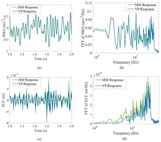
Figure 13.
Responses of the MM and the VP: (a) time response of the SMA; (b) frequency response of the SMA; (c) time response of the ECC; (d) frequency response of the ECC.
Table 4.
Modeling errors between the mathematical model and the VP model.
In the time domain, the VP model response is smaller than that of the MM for both the SMA and the ECC, with the feature being more obvious in SMA. Regarding the FFT comparison, the difference is noticeable at lower frequencies. When considering differences in the time and frequency domains, those might be caused by the tire rubber properties and the nonlinearity of the DVAS connector and the double cross arm.
Comparative results shown in Table 4 indicate that responses used in both models have an error lower than 10%. Since the error is within the permitted range [56], it was concluded that the proposed model is valid.
5. Conclusions
In this paper, an IVES was developed aiming to improve the vertical dynamics performance of the IWMD EVs in both sprung and unsprung conditions while also considering the UEMF effects. The mathematical model of the IVES was established, containing the DVAS-ASS integrated model and the novel FCT model. Moreover, the UEMF model during the driving maneuvers was also considered in the IVES model and was based on the theoretically analyzed UEMF effects. A delay-dependent controller was developed to improve the IVES performance by improving the ASS robustness to time delay. Finally, CATIA, ADAMS, and MATLAB/Simulink were used to create a virtual prototype environment needed to validate the accuracy and the practicability of the IVES.
Regarding the IVES performance, the numerical results obtained from the proposed mathematical model are consistent with the simulation results obtained from the virtual prototype. Compared to the passive suspension conditions, the RMS of sprung mass acceleration and the eccentricity are reduced via the IVES coordinated with the delay-dependent controller by up to 67.6% and 38.9%, respectively. The ride comfort is improved and the IWM vibration is suppressed, compensating for the adverse effects of UEMF on the vehicle vertical dynamics. In future work, the real time experimental validation of the IVES applied to the IWMD EVs will be conducted.
Author Contributions
Project administration, L.G. and J.W.; resources, L.G. and X.Z.; supervision, H.Y. and X.Z.; validation, L.G.; visualization, Z.Z.; data curation, Z.Z. and J.W.; writing—original draft, Z.Z. and X.Z.; writing—review and editing, Z.Z. and J.W. All authors have read and agreed to the published version of the manuscript.
Funding
This research was funded by the National Natural Science Foundation of China (Grant No. 52202457).
Institutional Review Board Statement
Not applicable.
Informed Consent Statement
The data involved in this paper do not involve ethical issues.
Data Availability Statement
The datasets used and analyzed during the current study are available from the corresponding author on reasonable request.
Conflicts of Interest
All authors certify that they have no affiliations with or involvement in any organization or entity with any financial interest or non-financial interest in the subject matter or materials discussed in this manuscript.
References
- Bilgin, B.; Liang, J.; Terzic, M.V.; Dong, J.; Rodriguez, R.; Trickett, E.; Emadi, A. Modeling and analysis of electric motors: State-of-the-art review. IEEE Trans. Transp. Electrif. 2019, 5, 602–617. [Google Scholar] [CrossRef]
- Wu, J.; Wang, Z.; Zhang, L. Unbiased-estimation-based and computation-efficient adaptive MPC for four-wheel-independently-actuated electric vehicles. Mech. Mach. Theory 2020, 154, 104100. [Google Scholar] [CrossRef]
- Luo, Y.; Tan, D. Research on the hub-motor driven wheel structure with a novel built-in mounting system. Automot. Eng. 2013, 35, 1105–1110. [Google Scholar]
- Kim, K.T.; Hwang, K.M.; Hwang, G.Y.; Kim, T.J.; Jeong, W.B.; Kim, C.U. Effect of rotor eccentricity on spindle vibration in magnetically symmetric and asymmetric BLDC motors. In Proceedings of the 2001 IEEE International Symposium on Industrial Electronics Proceedings (ISIE 2001), Pusan, Republic of Korea, 12–16 June 2001; Cat. No. 01TH8570. Volume 2, pp. 967–972. [Google Scholar]
- Ni, J.; Hu, J.; Xiang, C. A review for design and dynamics control of unmanned ground vehicle. Proc. Inst. Mech. Eng. Part D J. Automob. Eng. 2021, 235, 1084–1100. [Google Scholar] [CrossRef]
- Peng, H.; Wang, W.; An, Q.; Xiang, C.; Li, L. Path tracking and direct yaw moment coordinated control based on robust MPC with the finite time horizon for autonomous independent-drive vehicles. IEEE Trans. Veh. Technol. 2020, 69, 6053–6066. [Google Scholar] [CrossRef]
- Islam, R.; Husain, I. Analytical model for predicting noise and vibration in permanent-magnet synchronous motors. IEEE Trans. Ind. Appl. 2010, 46, 2346–2354. [Google Scholar] [CrossRef]
- Tan, D.; Lu, C. The influence of the magnetic force generated by the in-wheel motor on the vertical and lateral coupling dynamics of electric vehicles. IEEE Trans. Veh. Technol. 2015, 65, 4655–4668. [Google Scholar] [CrossRef]
- Liu, F.; Xiang, C.; Liu, H.; Han, L.; Wu, Y.; Wang, X.; Gao, P. Asymmetric effect of static radial eccentricity on the vibration characteristics of the rotor system of permanent magnet synchronous motors in electric vehicles. Nonlinear Dyn. 2019, 96, 2581–2600. [Google Scholar] [CrossRef]
- Kim, T.J.; Hwang, S.M.; Park, N.G. Analysis of vibration for permanent magnet motors considering mechanical and magnetic coupling effects. IEEE Trans. Magn. 2000, 36, 1346–1350. [Google Scholar]
- Qin, Y.; He, C.; Shao, X.; Du, H.; Xiang, C.; Dong, M. Vibration mitigation for in-wheel switched reluctance motor driven electric vehicle with dynamic vibration absorbing structures. J. Sound Vib. 2018, 419, 249–267. [Google Scholar] [CrossRef]
- Jin, L.; Yu, Y.; Fu, Y. Study on the ride comfort of vehicles driven by in-wheel motors. Adv. Mech. Eng. 2016, 8, 1687814016633622. [Google Scholar] [CrossRef]
- Xu, B.; Xiang, C.; Qin, Y.; Ding, P.; Dong, M. Semi-active vibration control for in-wheel switched reluctance motor driven electric vehicle with dynamic vibration absorbing structures: Concept and validation. IEEE Access 2018, 6, 60274–60285. [Google Scholar] [CrossRef]
- Qin, Y.; Wang, Z.; Yuan, K.; Zhang, Y. Comprehensive analysis and optimization of dynamic vibration-absorbing structures for electric vehicles driven by in-wheel motors. Automot. Innov. 2019, 2, 254–262. [Google Scholar] [CrossRef]
- Ma, Y.; Deng, Z.; Xie, D. Control of the active suspension for in-wheel motor. J. Adv. Mech. Des. Syst. Manuf. 2013, 7, 535–543. [Google Scholar] [CrossRef]
- Nagaya, G.; Wakao, Y.; Abe, A. Development of an in-wheel drive with advanced dynamic-damper mechanism. JSAE Rev. 2003, 24, 477–481. [Google Scholar] [CrossRef]
- Cseko, L.H.; Kvasnica, M.; Lantos, B. Explicit MPC-based RBF neural network controller design with discrete-time actual Kalman filter for semiactive suspension. IEEE Trans. Control. Syst. Technol. 2015, 23, 1736–1753. [Google Scholar] [CrossRef]
- Shieh, M.Y.; Chiou, J.S.; Liu, M.T. Design of immune-algorithm-based adaptive fuzzy controllers for active suspension systems. Adv. Mech. Eng. 2014, 6, 916257. [Google Scholar] [CrossRef]
- Sunwoo, M.; Cheok, K.C.; Huang, N. Model reference adaptive control for vehicle active suspension systems. IEEE Trans. Ind. Electron. 1991, 38, 217–222. [Google Scholar] [CrossRef]
- Chen, S.A.; Wang, J.C.; Yao, M.; Kim, Y.B. Improved optimal sliding mode control for a non-linear vehicle active suspension system. J. Sound Vib. 2017, 395, 1–25. [Google Scholar] [CrossRef]
- Badri, P.; Amini, A.; Sojoodi, M. Robust fixed-order dynamic output feedback controller design for nonlinear uncertain suspension system. Mech. Syst. Signal Process. 2016, 80, 137–151. [Google Scholar] [CrossRef]
- Marzbanrad, J.; Zahabi, N. H∞ active control of a vehicle suspension system exited by harmonic and random roads. Mech. Mech. Eng. 2017, 21. [Google Scholar]
- Sun, W.; Gao, H.; Yao, B. Adaptive robust vibration control of full-car active suspensions with electrohydraulic actuators. IEEE Trans. Control. Syst. Technol. 2013, 21, 2417–2422. [Google Scholar] [CrossRef]
- Choi, S.B.; Han, S.S. H∞ control of electrorheological suspension system subjected to parameter uncertainties. Mechatronics 2003, 13, 639–657. [Google Scholar] [CrossRef]
- Li, H.; Gao, H.; Liu, H. Robust quantised control for active suspension systems. LET Control. Theory Appl. 2011, 5, 1955–1969. [Google Scholar] [CrossRef]
- Shao, X.; Naghdy, F.; Du, H. Reliable fuzzy H∞ control for active suspension of in-wheel motor driven electric vehicles with dynamic damping. Mech. Syst. Signal Process. 2017, 87, 365–383. [Google Scholar] [CrossRef]
- Jing, H.; Wang, R.; Li, C.; Wang, J.; Chen, N. Fault-tolerant control of active suspensions in in-wheel motor driven electric vehicles. Int. J. Veh. Des. 2015, 68, 22–36. [Google Scholar] [CrossRef]
- Shoukry, Y.; El-Shafie, M.; Hammad, S. Networked embedded generalized predictive controller for an active suspension system. In Proceedings of the 2010 American Control Conference, Baltimore, MD, USA, 30 June–2 July 2010; pp. 4570–4575. [Google Scholar]
- Liu, M.; Zhang, Y.; Huang, J.; Zhang, C. Optimization control for dynamic vibration absorbers and active suspensions of in-wheel-motor-driven electric vehicles. Proc. Inst. Mech. Eng. Part D J. Automob. Eng. 2020, 234, 2377–2392. [Google Scholar] [CrossRef]
- Wang, R.; Jing, H.; Yan, F.; Karimi, H.R.; Chen, N. Optimization and finite-frequency H∞ control of active suspensions in in-wheel motor driven electric ground vehicles. J. Frankl. Inst. 2015, 352, 468–484. [Google Scholar] [CrossRef]
- Liu, M.; Gu, F.; Huang, J.; Wang, C.; Cao, M. Integration design and optimization control of a dynamic vibration absorber for electric wheels with in-wheel motor. Energies 2017, 10, 2069. [Google Scholar] [CrossRef]
- Li, Z.; Zheng, L.; Gao, W.; Zhan, Z. Electromechanical coupling mechanism and control strategy for in-wheel-motor-driven electric vehicles. IEEE Trans. Ind. Electron. 2018, 66, 4524–4533. [Google Scholar] [CrossRef]
- Jin, L.; Song, C.; Wang, Q. Evaluation of Influence of Motorized Wheels on Contact Force and Comfort for Electric Vehicle. J. Comput. 2011, 6, 497–505. [Google Scholar] [CrossRef]
- Deur, J.; Asgari, J.; Hrovat, D. A 3D brush-type dynamic tire friction model. Veh. Syst. Dyn. 2004, 42, 133–173. [Google Scholar] [CrossRef]
- Besselink, I.; Schmeitz, A.; Pacejka, H. An improved Magic Formula/Swift tyre model that can handle inflation pressure changes. Veh. Syst. Dyn. 2010, 48, 337–352. [Google Scholar] [CrossRef]
- Zegelaar, P.; Pacejka, H. Dynamic tyre responses to brake torque variations. Veh. Syst. Dyn. 1997, 27, 65–79. [Google Scholar] [CrossRef]
- Gipser, M. FTire: A physically based application-oriented tyre model for use with detailed MBS and finite-element suspension models. Veh. Syst. Dyn. 2005, 43, 76–91. [Google Scholar] [CrossRef]
- Mao, Y.; Zuo, S.; Wu, X.; Duan, X. High frequency vibration characteristics of electric wheel system under in-wheel motor torque ripple. J. Sound Vib. 2017, 400, 442–456. [Google Scholar] [CrossRef]
- Anwar, M.; Husain, I. Radial force calculation and acoustic noise prediction in switched reluctance machines. IEEE Trans. Ind. Appl. 2000, 36, 1589–1597. [Google Scholar] [CrossRef]
- Jokinen, T.; Hrabovcova, V.; Pyrhonen, J. Design of Rotating Electrical Machines; John Wiley & Sons: Hoboken, NJ, USA, 2013. [Google Scholar]
- Zhu, W.; Pekarek, S.; Fahimi, B.; Deken, B.J. Investigation of force generation in a permanent magnet synchronous machine. IEEE Trans. Energy Convers. 2007, 22, 557–565. [Google Scholar] [CrossRef]
- Xue, X.; Cheng, K.W.E.; Lin, J.; Zhang, Z.; Luk, K.; Ng, T.W.; Cheung, N.C. Optimal control method of motoring operation for SRM drives in electric vehicles. IEEE Trans. Veh. Technol. 2010, 59, 1191–1204. [Google Scholar] [CrossRef]
- Ebrahimi, B.M.; Faiz, J.; Roshtkhari, M.J. Static-, dynamic-, and mixed-eccentricity fault diagnoses in permanent-magnet synchronous motors. IEEE Trans. Ind. Electron. 2009, 56, 4727–4739. [Google Scholar] [CrossRef]
- Qin, Y.; Wang, Z.; Xiang, C.; Hashemi, E.; Khajepour, A.; Huang, Y. Speed independent road classification strategy based on vehicle response: Theory and experimental validation. Mech. Syst. Signal Process. 2019, 117, 653–666. [Google Scholar] [CrossRef]
- Qin, Y.; Wei, C.; Tang, X.; Zhang, N.; Dong, M.; Hu, C. A novel nonlinear road profile classification approach for controllable suspension system: Simulation and experimental validation. Mech. Syst. Signal Process. 2019, 125, 79–98. [Google Scholar] [CrossRef]
- ISO 8608:1995; Mechanical Vibration–Road Surface Profiles–Reporting of Measured Data. International Organization for Standardization: Geneva, Switzerland, 1995; Volume 8608.
- Canudas-de Wit, C.; Tsiotras, P.; Velenis, E.; Basset, M.; Gissinger, G. Dynamic friction models for road/tire longitudinal interaction. Veh. Syst. Dyn. 2003, 39, 189–226. [Google Scholar] [CrossRef]
- Ozerem, O.; Morrey, D. A brush-based thermo-physical tyre model and its effectiveness in handling simulation of a Formula SAE vehicle. Proc. Inst. Mech. Eng. Part D J. Automob. Eng. 2019, 233, 107–120. [Google Scholar] [CrossRef]
- Guo, Z.; Wu, W.; Yuan, S. Longitudinal-vertical dynamics of wheeled vehicle under off-road conditions. Veh. Syst. Dyn. 2022, 60, 470–490. [Google Scholar] [CrossRef]
- Karnopp, D. How significant are transfer function relations and invariant points for a quarter car suspension model? Veh. Syst. Dyn. 2009, 47, 457–464. [Google Scholar] [CrossRef]
- Tseng, H.E.; Hrovat, D. State of the art survey: Active and semi-active suspension control. Veh. Syst. Dyn. 2015, 53, 1034–1062. [Google Scholar] [CrossRef]
- Tuononen, A.; Hartikainen, L.; Petry, F.; Westermann, S. Parameterization of in-plane rigid ring tire model from instrumented vehicle measurements. In Proceedings of the 11th International Symposium on Advanced Vehicle Control (AVEC’12), Seoul, Republic of Korea, 9–12 September 2012; pp. 9–12. [Google Scholar]
- Apkarian, P.; Tuan, H.D.; Bernussou, J. Continuous-time analysis, eigenstructure assignment, and H/sub 2/synthesis with enhanced linear matrix inequalities (LMI) characterizations. IEEE Trans. Autom. Control. 2001, 46, 1941–1946. [Google Scholar] [CrossRef]
- Cottle, R.W. Manifestations of the Schur complement. Linear Algebra Its Appl. 1974, 8, 189–211. [Google Scholar] [CrossRef]
- Guo, L.X.; Zhang, L.P. Robust H∞ control of active vehicle suspension under non-stationary running. J. Sound Vib. 2012, 331, 5824–5837. [Google Scholar] [CrossRef]
- Guiggiani, M. The Science of Vehicle Dynamics; Springer: Dordrecht, The Netherlands, 2014; p. 15. [Google Scholar]


Disclaimer/Publisher’s Note: The statements, opinions and data contained in all publications are solely those of the individual author(s) and contributor(s) and not of MDPI and/or the editor(s). MDPI and/or the editor(s) disclaim responsibility for any injury to people or property resulting from any ideas, methods, instructions or products referred to in the content. |
© 2023 by the authors. Licensee MDPI, Basel, Switzerland. This article is an open access article distributed under the terms and conditions of the Creative Commons Attribution (CC BY) license (https://creativecommons.org/licenses/by/4.0/).