Task Scheduling Based on Adaptive Priority Experience Replay on Cloud Platforms

Abstract

Task scheduling algorithms based on reinforce learning (RL) have been important methods with which to improve the performance of cloud platforms; however, due to the dynamics and complexity of the cloud environment, the action space has a very high dimension. This not only makes agent training difficult but also affects scheduling performance. In order to guide an agent’s behavior and reduce the number of episodes by using historical records, a task scheduling algorithm based on adaptive priority experience replay (APER) is proposed. APER uses performance metrics as scheduling and sampling optimization objectives with which to improve network accuracy. Combined with prioritized experience replay (PER), an agent can decide how to use experiences. Moreover, this algorithm also considers whether a subtask is executed in a workflow to improve scheduling efficiency. Experimental results on Tpc-h, Alibaba cluster data, and scientific workflows show that a model with APER has significant benefits in terms of convergence and performance.

1. Introduction

Cloud computing is one of the hot spots in the field of information and communication technology. Its pay-as-you-go mode is favored by users. Task scheduling on cloud platforms refers to allocating computing resources to corresponding tasks by using appropriate scheduling rules. To improve service quality, the average response time of tasks should be reduced; however, with the continuous development of cloud computing the number of tasks is constantly changing and the dependence between tasks is increasingly complex, so designing a reasonable scheduling scheme is a problem that deserves further research.

Task scheduling algorithms on cloud platforms include traditional algorithms, heuristic algorithms, and reinforce learning (RL). Traditional algorithms [1,2] are easy to understand and implement, but difficult to be tuned and improved. They do not consider the dynamics and complexity of current cloud platform tasks, especially workflows, which are a kind of task with dependency. Scheduling a cloud workflow is an NP-hard problem [2], and a heuristic algorithm is the main method with which to solve it.

Heuristic algorithms can be divided into two categories according to their characteristics: Static ones [3,4,5,6] are generally simple strategies and are suitable for tasks that are known before scheduling. Dynamic algorithms [7,8,9] consider the dynamics of cloud platforms, but there are some problems, such as a large number of iterations and long computation times [9,10,11]. In addition, though static and dynamic algorithms can both deal with tasks with dependency [5,6,8,12,13,14], dependency also brings task validity issues [15].

Compared with heuristics, scheduling based on RL can learn offline and infer online, which overcome the shortcomings of heuristics. RL can directly learn scheduling policies from historical experience without relying on human experience [16,17,18,19,20]; however, RL for scheduling decisions usually uses all of the experiences in the buffer. These methods cannot distinguish the influence of different experiences on the overall model, such that the learning efficiency is low.

To address the low learning efficiency, we propose a cloud platform task scheduling algorithm based on the adaptive prioritized experience replay (APER) strategy. APER can adaptively decide which experience to be used can update a model better and faster, combining the dynamic adjustment strategy based on PER. In this paper, the performance metric is used as the scheduling and sampling optimization objective with which to improve the accuracy of a network. Moreover, a selection function is added to ensure that the action space only contains executable tasks. After the above, the model is validated on task scheduling datasets with different scenarios. Experiments show that the model with APER converges faster and the task completion time is shorter. The main contributions of this paper can be summarized as follows:

(1)

We propose an adaptive priority experience replay (APER) strategy, which can dynamically adjust the sampling strategy. This improves convergence speed and performance.

(2)

We adopt new optimization objectives and selection functions. The scheduling objective is unified with the sampling optimization objective. Additionally, the selection functions can avoid invalid scheduling actions.

(3)

We test APER on workflow scheduling datasets in different scenarios. Our results demonstrate that APER performs well on real-world datasets. The advantage becomes more significant using datasets with more diversity.

The remainder of this paper is structured as follows: Section 2 presents the related work. Section 3 introduces important components and the scheduling model. Section 4 presents the details of the proposed APER approach with implementation. Section 5 reports the experimental results, and Section 6 concludes this paper.

2. Related Work

2.1. Reinforce Learning

RL [21,22] learns policies by interacting with the environment. The environment will switch to a new state according to the agent’s action and return the reward of the action. The agent then performs the next actions according to a strategy based on the new state. In this process, an agent can directly learn which actions are performed in different states to obtain the maximum cumulative reward.

According to the task type, task scheduling algorithms can be divided into independent task scheduling and dependent task scheduling. There have been many RL algorithms based on independent task scheduling, such as DSS (DRL&LSTM) [23], DQN [24,25,26,27,28,29], AC [30], DeepJS [2], DeepRM [31], DRL&Transformer [32], PPO [33], A2C [34], double DQN [35], hierarchical DRL [36], RL&Game-theory [37], and so on. These RL algorithms achieve good results. Mitsis et al. [37] propose a task scheduling framework based on RL and game theory, exploiting tasks’ and then end nodes’ characteristics in order to perform task scheduling and execution while considering user risk-aware decision-making behavior to maximize user satisfaction and the benefit of service providers. Cheng et al. [28] propose a cost-aware and real-time cloud task scheduling model based on RL, showing a significant reduction in the execution cost as well as the average response time. Considering QoS, Yan et al. [29] propose a real-time task scheduling algorithm based on RL, which minimizes energy costs.

However, most independent task scheduling algorithms only consider the fact that tasks arrive immediately and order the tasks, without involving dependencies. With the development of cloud platforms, task scheduling with dependencies has gradually become a research hotspot, and these tasks are usually abstracted as DAGs. In recent years, there have been many studies on DAG scheduling strategies using RL, and some results have been achieved.

There have been many studies on static DAG scheduling. Souri et al. [38] considered the types of nodes, the social relationships and trust between nodes, and proposed a trust-based friend selection strategy for cooperative processing tasks. Their method was also a game between the best cooperative node and the shortest network distance, after which the node execution order was planned.

Only a few studies use RL, and they usually involve learning a fixed strategy. Long et al. [39] proposed an improved self-learning artificial bee colony (SLABC) algorithm based on RL to solve the problems of a slow convergence speed and reaching a local optimum in ABC. Paszke et al. [40] used RL to guide a genetic algorithm to optimize the execution cost of neural network computation graphs. Gao et al. [41] modeled the node scheduling process in DAG as a Markov decision process with PPO. In [42], DRL was employed to learn local search heuristics for solving DAG problems. This algorithm does not extend to larger or smaller DAGs. The scheduling strategy is static, and the environment is deterministic. Both of them are important limitations to practical constraints in dynamic environments.

Compared with static algorithms, there are more studies on dynamic DAG scheduling algorithms with RL. Bao et al. [43] proposed Harmony, a dynamic deep learning cluster scheduler that considers the relationships between tasks, using job-aware action space exploration with experience replay. Lee et al. [44] proposed a DAG scheduling algorithm based on RL, which automatically identifies critical temporal and graph structural features in order to assign each task in a single DAG. Hu et al. [45] proposed Spear, which considers task dependencies, utilizing Monte Carlo tree search (MCTS) and DRL to guide complex DAG scheduling. Some research [46,47] use RL network based on RNN to generate scheduling strategies which utilize the dependencies as the input information of this network. Zhu et al. [48] propose a workflow scheduling algorithm in order to solve task combination and resource selection, which allocates appropriate virtual machine resources for each task in the workflow, scheduling workflow by a genetic algorithm, and learning real-time scheduling policy by RL; however, it is difficult for these algorithms to utilize DAG information flexibly and fully.

In order to extract more graph information, researchers add graph neural networks (GNNs [49]) to deal DAGs, inspired by the powerful graph processing capabilities of GNNs. Zhang et al. [50] proposed automatically learning a scheduling strategy via an end-to-end DRL and GNN to embed the states encountered during solving, which does not depend on the size of a DAG. Sun et al. [51] proposed DeepWeave, which employs GNNs to process DAG information and RL to train, improving the scheduling ability in DAGs. Grinsztajn et al. [52] combine GNNs with the A2C algorithm in order to build an adaptive representation of the scheduling problem and learn scheduling strategies. Mao et al. [10] use scalable GNNs to extract DAG features and design a dynamic DAG scheduler based on RL by using batch training, which achieves remarkable results in single scene.

These algorithms optimize the task completion time of DAG scheduling, but some of them pay insufficient attention to whether a node is executable. For the purpose of a convenient description, this paper calls this “executability” [15]. This will affect task completion times and training effects. Furthermore, these algorithms do not pay attention to experience utilization efficiency. Some studies have shown that it is possible to improve experience utilization and performance via prioritized experience replay (PER) [53].

2.2. Prioritized Experience Replay

Neuroscience has established that, in rodents, experience is learned repeatedly during rest or sleep. Experience has found that reward-related experience sequences are used more frequently [54]. Inspired by this, many prioritized sampling strategies on buffers have emerged, which are beneficial to improving experience utilization efficiency and the performance of agents. Schaul et al. [55] proposed PER which judges the importance of experience through TD error. In training, agent prefers to use experience with high TD error. Although this strategy improves model performance and experience utilization efficiency, it loses the diversity of samples, which may lead to instability [56]. Wang et al. [53] believe that the newly collected experience is more important. They proposed the emphasizing recent experience (ERE) strategy, which is consistent with more accurate human recent memory and vaguer long-term memory. It achieves better results on MuJoCo. Kumar et al. [56,57] estimated Q value more accurately and judged experience’s importance, reducing the instability brought by a network itself. Kumar et al. [56] believe that an algorithm’s performance will be affected when the optimization objective of a sampling strategy is different from that of an agent. Liu et al. [57] verified this conclusion. To solve this problem, they proposed two new algorithms that consider large TD error experience based on maximizing the Q value. Additionally, they verified algorithms’ performance with standard off-policy RL.

These strategies sample experience by calculating its importance; however, always using part of experience leads to instability [58].

3. Method

For convenient description and experimentation, we make the following assumptions: First, it is assumed that all of the hardware resources in cloud platforms are the same and that the computing resources are only divided according to the number of CPUs, which are called executors. Second, executors are restricted from being preempted and shared until tasks on these executors are finished. Finally, this paper focuses on dynamic and randomly arriving DAG task scheduling. An independent task will be regarded as a DAG with only one node and without an edge. Table 1 shows the descriptions of symbols in DAG scheduling problems.

Table 1. Descriptions of symbols in DAG scheduling problems.

Symbol	Description	Symbol	Description
$N$	All nodes in a DAG	${\mathit{e}}_n^{G_m}$	The feature of a node
$N_n$	$n$$\text{-}\mathrm{th}\mathrm{node}\mathrm{in}N$$,1\le n\le N$	${\mathit{e}}^{G_m}$	The feature of a DAG
$E$	All edges in a DAG	${\mathit{e}}^G$	The feature of global
$E_{ij}$	$\mathrm{Edge}\mathrm{from}{N}_i$$\mathrm{to}{N}_j$, $N_i,N_j\in N$	$r_t$	$t$th step reward
$A\left(G\right)$	A $n\times n$$\mathrm{adjacency}\mathrm{matrix}\mathrm{to}\mathrm{represent}\mathrm{the}\mathrm{edge}\mathrm{in}N$	$\gamma$	Discount factor
$M$	The set of DAGs	$R_t$	$\mathrm{The}\mathrm{cumulative}\mathrm{reward}\mathrm{from}\mathrm{the}t$th step
$G_m$	$m$-th DAG, $1\le m\le M$	$p\left(e\right)$	The filter for executability
$N_n^{G_m}$	n-th node in the m-th DAG	$sr$	The sample rate
$AFT\left(·\right)$	The actual finish time (metric: ms)	$Ad{v}_t$	$\mathrm{The}\mathrm{advantage}\mathrm{of}\mathrm{the}t\mathrm{th}\mathrm{action}\mathrm{by}{R}_t$
$AST\left(·\right)$	The actual start execution time (metric: ms)	$f\left(·\right),g\left(·\right)$	Non-linear functions
$AUT\left(·\right)$	The completion time (metric: ms)	$\mathsf{\theta }$	The model parameters
$V$	The number of available executors	${\pi }_{\theta }$	$\mathrm{The}\mathrm{policy}\mathrm{with}\mathsf{\theta }$
$c_v$	The state of executors; available is 1, else 0	$En{t}_{{\pi }_{\theta }}\left(·\right)$	The policy entropy
$G_m^{cpu}$	$\mathrm{The}\mathrm{current}\mathrm{CPU}\mathrm{number}\mathrm{of}{G}_m$	$w_e$	The weight of the policy entropy
$Av{g}_{JCT}$	The average JCT of all DAGs (metric: ms)	${\mathrm{L}}_{{\pi }_{\theta }}\left(s_t,a_t\right)$	$\mathrm{The}\mathrm{loss}\mathrm{function}\mathrm{of}(s_t,a_t)$

3.1. Related Definitions

DAG. This paper abstracts interdependence tasks into DAGs [59]. The formal description is as follows:

$$G=(N,E)$$

(1)

Equation (1) satisfies the following:

(1)

The node set, $N=\left\{N_n|1\le n\le N\right\}$, represents different types of tasks in a DAG.

(2)

The edge set, $E=\left\{E_{ij}=\left(N_i,N_j\right)|N_i,N_j\in N\right\}$, represents a directed edge from node $N_i$ to node $N_j$, reflecting the dependencies between tasks and using an adjacency matrix, $A\left(G\right)={\left[\left(N_i,N_j\right)\right]}_{n\ast n}$, representation, $\left(N_i,N_j\right)=\left\{\begin{array}{c}1if(N_i,N_j)\in E\\ 0if\left(N_i,N_j\right)\notin E\end{array}\right.$.

(3)

For any sequence, $\{\left(N_{n_1},N_{n_2}\right),\left(N_{n_2},N_{n_3}\right),\left(N_{n_3},N_{n_4}\right),\dots ,\left(N_{n_{k-2}},N_{n_{k-1}}\right),\left(N_{n_{k-1}},N_{n_k}\right)\}$ satisfies $N_{n_1}\ne N_{n_k}$.

Figure 1 shows a DAG example. Node 1 is the predecessor of 2, and 2 is the successor of 1, so 1 is always executed before 2. Nodes 2 and 3 have no dependencies and can be parallelized, so they belong to the same stage. Dividing stages is beneficial for assigning multiple executors to a DAG in the same stage to improve the efficiency of DAG execution.

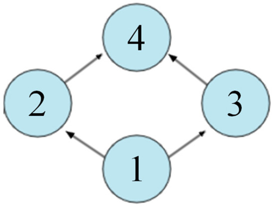
Figure 1. A DAG example.

In this paper, $M=\left\{G_m|1\le m\le M\right\}$ represents the set of randomly arriving DAGs. $G_m$ is the $m$-th DAG. $G_m^{cpu}$ is the current CPU number of $G_m$. $AFT\left(G_m\right)$ is the actual finish time of $G_m$. $AST\left(G_m\right)$ is the actual start execution time of $G_m$.

The completion time of $G_m$ is as follows:

$$AUT\left(G_m\right)=AFT\left(G_m\right)-AST\left(G_m\right)$$

(2)

The average job completion time (JCT) of all DAGs is defined as shown in Equation (3). The objective of this paper is to minimize $Av{g}_{JCT}$:

$$Av{g}_{JCT}=\frac{{\sum }_{G_m\in M}AUT\left(G_m\right)}{M}$$

(3)

For $N=\left\{N_n^{G_m}\right|1\le n\le N\}$, calculating the completion time of each node is performed as follows:

$$AUT\left(N_n^{G_m}\right)=AFT\left(N_n^{G_m}\right)-AST\left(N_n^{G_m}\right)$$

(4)

$AFT\left(N_n^{G_m}\right)$ is the actual finish time of $G_m$. $AST\left(N_n^{G_m}\right)$ is the actual start execution time of $G_m$. $AUT\left(G_m\right)$ and $AUT\left(N_n^{G_m}\right)$ include scheduling time and execution time. Node $N_n^{G_m}=(AUT\left(N_n^{G_m}\right),{task\_num}_n^{G_m})$, where ${task\_num}_n^{G_m}$ is the number of tasks on node $n$. The actual completion time of a DAG is the maximum value of all of the nodes’ actual completion times on a DAG:

$$AFT\left(G_m\right)=Max\left(AFT\left(N_n^{G_m}\right)\right),1\le n\le N$$

(5)

$Makespan=Max\left(AFT\left(G_m\right)\right)$ represents the total time spent on scheduling, $m$, using a certain strategy. It is the maximum of all of the nodes’ actual completion times.

During the scheduling process, it is necessary to ensure that the sum number of executors allocated to all DAGs does not exceed the maximum number of CPUs, $V$, in the cluster, which satisfies the resource constraints of the cluster:

$$\sum _{m=1}^M{G}_m^{cpu}\le V$$

(6)

3.2. Important Components

This paper uses RL to implement DAG task scheduling. Some important components are described as follows:

Agent. The main body that makes scheduling decisions, which outputs action by observing the current cloud platform state. After an action is executed the environment generates a reward for action and transfers to a new state.

State space. Observes environment information by an agent after executing action. The state space size depends on the number of available executors and the number of nodes to be scheduled. In this paper, whenever a scheduling event is triggered the environment updates available executor information and the task information to be scheduled. The number of available executors is represented by a vector, $\mathit{c}=\left\{c_v|1\le v\le V\right\}$. The task information to be scheduled is represented as executable nodes in each DAG. These nodes use a vector, $[node\_id,job\_id,druation\_time,task\_num,stage\_num]$, as the input state, where $node\_id$ and $job\_id$ represent the node ID and DAG ID to which a node belongs, $druation\_time$ represents the completion time of a node, $AUT\left(N_n^{G_m}\right)$, $task\_num$ is the task number for a node, $n$, in $G_m$ (${task\_num}_n^{G_m}$), and $stage\_num$ is the node stage.

Action space. An agent selects an executable node in each scheduling process, while also specifying the maximum number of executors for a DAG where the node is located. They are defined as action vectors, $[\mathit{n}\mathit{o}\mathit{d}\mathit{e},\mathit{p}\mathit{a}\mathit{r}\mathit{a}\mathit{l}]$. The action space size is limited by the number of available executors and the number of nodes to be scheduled. If there are fewer executors and more nodes, the agent will wait until the DAG execution ends and the executors are released. If there are fewer nodes and more executors, the agent will allocate more executors to the selected node to reduce the execution time.

Reward. RL uses a reward to gradually improve the scheduling policy. Every time an action is performed, an agent receives a reward, $r$, generated by the environment. Since agents cannot know the impact of current behavior on the future in a short period, there may be a situation where the current behavior reward is low but the overall result is better. Therefore, this work takes the cumulative reward, $R$, as the optimization objective. Equation (7) shows how to obtain $R_t$ by using the $r$ of the $t$-th to $(t+k)$-th steps represented by [$r_t,r_{t+1},\dots ,r_{t+k}$], where $\gamma$ is the discount factor denoting the impact of future actions on the current action, and is set to 0.9 in this paper:

$$R_t=r_t+\gamma r_{t+1}+{\gamma }^2{r}_{t+2}+\dots =\sum _{k=0}^{\mathrm{\infty }}{\gamma }^k{r}_{t+k}$$

(7)

In the field of task scheduling the objective is JCT, and Equations (2)–(5) reflect the impact of node scheduling time on JCT. This being the case, the node scheduling time is used as $r$. Assuming that two adjacent scheduling actions are generated at $t_k$ and $t_{k+1}$, the $r_t$ is set to $-\left(t_{k+1}-t_k\right)$, which reflects JCT in the event-triggered scheduler. Combined with Equation (7), define $R_t$ as shown in Equation (8). An agent achieves the optimization objective by maximizing $R_t$:

$$R_t=-{\sum }_{k=0}^k\left(t_{k+1}-t_k\right){\gamma }^k$$

(8)

An agent’s performance will be affected by the difference between the scheduling optimization objective and the sampling optimization objective. This paper takes $R_t$ as the optimization objective of the sampling strategy to reduce the effect.

Buffer. Used to store experience from each scheduling, including state, action, reward, etc. It helps to break down temporal correlations between experiences, reuse experiences, and reduce learning costs [60].

3.3. Model Structure

Figure 2 shows the model’s structure. The cloud platform is regarded as the environment. The DAG and cluster resources are represented as the state. A GNN aggregates the features from the state. A policy network selects the action via the features. After executing a scheduling action, the environment updates the state and reward. The buffer stores the state, action, and reward to train offline. This part is described in Section 4.1.

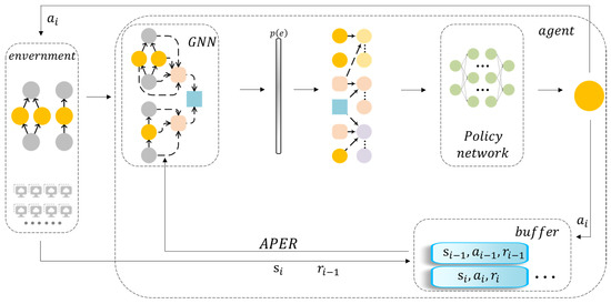
Figure 2. Model framework.

When the buffer reaches the upper limit of capacity, or all DAGs are finished, the model will be updated. Experiences are selected according to the sample rate using APER after calculating the reward. These experiences are used to compute new scheduling actions and sample rates. This model will then be updated by using policy gradient methods. This part is described in Section 4.2.

4. Implementation

4.1. Task Scheduling

The state space will be updated when a scheduling event is triggered. Since the sequence and processing time of each task are unknown, it is impossible to update the state space frequently by using the strategy in [61]. Whenever a node is set to be changed the state space is updated and a scheduling action is triggered. Specifically, scheduling events occur when (i) DAGs finish executing, and the executor is released; (ii) a stage is completed and its substages need to be executed; and (iii) a new DAG arrives. In this paper, a DAG randomly arrives to ensure that an agent does not acquire prior knowledge before DAG arrivals, but instead completely relies on the scheduling strategy to make decisions.

Extracting DAG features needs to consider their structural information; however, different DAGs have different sizes, which brings difficulties to feature extraction. The authors of [6,13] use the adjacency matrix of a DAG to extract features by splitting a DAG. This method loses a DAG’s partial dependency information. This paper uses a GNN [10,20,49] to implement a scale feature extraction network [62] that can directly embed dependency information into node features. In Figure 3, the GNN uses the parameter information of each node and its predecessor nodes to extract node features. Equation (9) shows the method for computing node features:

$${\mathit{e}}_n^{G_m}=g_1\left({\sum }_{n^{\prime }\in \phi \left(n\right)}{f}_1\left({\mathit{e}}_{n^{\prime }}^{G_m}\right)\right)+{\mathit{N}}_n^{G_m}$$

(9)

where ${\mathit{e}}_n^{G_m}$ is the feature of node n. ${\mathit{N}}_n^{G_m}$ is the original information of n. $\phi \left(n\right)$ is the predecessor node set of n. $f_1\left(·\right)$ and $g_1\left(·\right)$ are different non-linear functions. All nodes’ features in each DAG are used to extract DAG features in Equation (10), and global features are synthesized through global DAG features in Equation (11):

$${\mathit{e}}^{G_m}=g_2\left({\sum }_{n\in G_m}{f}_2\left({\mathit{e}}_n^{G_m}\right)\right)$$

(10)

$${\mathit{e}}^G=g_3\left({\sum }_{G_m\in M}{f}_3\left({\mathit{e}}^{G_m}\right)\right)$$

(11)

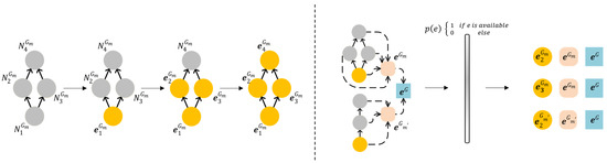
Figure 3. Extracting DAG features.

${\mathit{e}}^{G_m}$ is the feature of $G_m$ and ${\mathit{e}}^G$ is the global feature. $f_2\left(·\right)$, $g_2\left(·\right)$, $f_3\left(·\right)$, and $g_3\left(·\right)$ are non-linear functions, such as $f_1\left(·\right)$ and $g_1\left(·\right)$.

However, task dependencies may cause agents to select invalid nodes [10,15,20], such as nodes that have already been executed or whose predecessor nodes have not yet been completed. Although this problem can be solved by rescheduling, it may lead to task accumulation, which will increase platform burden. To solve this problem, this paper adds a filter, $p\left(e\right)$ (in Equation (12)), after extracting features. The node may be selected only when ${\mathit{e}}_n^{G_m}\times p\left(e\right)\ne 0$ (in Equation (13)). This method only sends the node features that meet scheduling conditions into the policy network, which not only ensures task validity but also reduces state space size:

$$p\left(e\right)=\left\{\begin{array}{cc}1& if e is available\\ 0& else\end{array}\right.$$

(12)

$${\mathit{e}}_n^{G_m},{\mathit{e}}^{G_m},{\mathit{e}}^G\leftarrow \left({\mathit{e}}_n^{G_m},{\mathit{e}}^{G_m},{\mathit{e}}^G\right)\times p\left(e\right)$$

(13)

At this time, the state space is represented as three parts: a DAG set, $M=\left\{G_m\right|1\le m\le M\}$; the available node set, $N=\left\{N_n\right|1\le n\le N\}$, of each DAG; and parameters, $N_n^{G_m}=(druation\_time,task\_num,exe\_num)$, within each node, where $exe\_num$ is the executor number of $G_m$.

Extracted features are passed to the policy network. The policy network consists of two parts: The first part uses node features and DAG features as inputs with which to calculate the scheduling probability of each node. Agents will select the highest probability node to execute a scheduling action. The second part inputs DAG features and global features, which are used to calculate the probability of the parallelism level for each DAG. The number of output layers is V. Agents assign the maximum number of executors to the target node by using the degree of parallelism with the maximum probability. They are $[\mathit{n}\mathit{o}\mathit{d}\mathit{e},\mathit{p}\mathit{a}\mathit{r}\mathit{a}\mathit{l}]$. Scheduling decisions in real scenarios need to estimate $AUT\left(N_n^{G_m}\right)$ as accurately as possible based on historical data but use the complete time provided by a dataset during training.

After executing a scheduled action, the environment produces a reward and the next state. Agents retain $AFT\left(N_n^{G_m}\right)$ to calculate $AFT\left(G_m\right)$. The state, action, and reward are stored, while the next batch of nodes is scheduled and executed. $Av{g}_{JCT}$ will be calculated after all of the nodes in a DAG are completed, as shown in Equation (3).

4.2. Adaptive Priority Experience Replay

After all DAGs are executed or the buffer capacity reaches the upper limit, the model will be optimized. This paper uses JCT as the performance metric with which to calculate the agent scheduling objective and sample optimization objective. The sample rate, $sr$, is determined by the policy network. The efficiency of experience utilization is improved by gradually expanding from a small amount of good experience to the whole experience, thereby improving convergence speed and model performance [58]. In the optimization process, the GNNs and filters are the same as those in Section 4.1.; only the policy network adds a fully connected network in order to calculate the sample rate.

First, this paper sets $sr\in \{0.1,0.2,0.3,0.4,0.5,0.6,0.7\}$ to reduce the action space. The highest probability level is chosen as the $sr$ at each episode. The $sr$ is utilized to select experience. At the beginning of training, the $sr$ will be initialized randomly. The new action and $sr$ are then calculated by the policy network. Since each experience will calculate an $sr$, before the end of each episode the model will select the highest frequency $sr$ as the real $sr$ of the next episode. In Equation (14), $s{r}_i$ is the sample rate of different levels:

$$sr=\underset{s{r}_i}{\mathrm{argmax}}\left(\frac{count\left(s{r}_i\right)}{\sum count\left(s{r}_i\right)}\right)$$

(14)

The advantage of the current agent is calculated at time t by using Equation (15), after which a high $Adv$ experience is defined as the good experience and the other is the poor one. The neural network adaptively adjusts the importance of the two types of experience. It guides the model to use a small amount of good experience first, after which it gradually expands to use all experience. The advantage of this method is that when the model uses a small amount of good experience it can speed up the model convergence; when using a large amount of experience it can avoid the model from falling into a local optimum. Because all experience is still used in the end, the bias in sampling is reduced. $baseline\left(R_t\right)$ is derived from the average $R_t$ of all trained agents [63]:

$$Ad{v}_t=\sum _t{R}_t-baseline\left(R_t\right)$$

(15)

In Equation (16), experience $t$ will be selected if $t$ is the top $sr$ of the buffer. Good experience is beneficial for accelerating convergence, but bad experience should not be forgotten [64]. While using good experience, this paper randomly selects some instances of bad experience from the remaining experience (in Algorithm 1). As the training progresses, the model expands the selected experience scope from a small amount of good experience to a large amount of experience; it will also adaptively adjust the sample rate in the process until all experience is used:

$${Adv}_t=\left\{\genfrac{}{}{0pt}{}{{Adv}_t}{null}\genfrac{}{}{0pt}{}{if Ad{v}_t is the top sr and the end s{r}^2}{else}\right.$$

(16)

Finally, the model parameters, $\mathsf{\theta }$, will be updated using ${Adv}_t$ in Equation (17) and Equation (18), where ${\pi }_{\theta }$ represents the current policy; $\mathsf{\alpha }=0.01$ is the learning rate; $En{t}_{{\pi }_{\theta }}\left(a_t\right)$ is the policy entropy of using $a_t$ for policy ${\pi }_{\theta }$; the higher the probability of action, $a_t$, the higher the accuracy of the decision and the smaller $En{t}_{{\pi }_{\theta }}\left(a_t\right)$; and $w_e$ represents the weight of policy entropy, decreased from 1 to 0.01. We want the dominance term, $\mathrm{l}\mathrm{o}\mathrm{g}{\pi }_{\theta }\left(s_t,a_t\right)Ad{v}_t$, to be larger, and the policy entropy term, $w_e\times En{t}_{{\pi }_{\theta }}\left(a_t\right)$, to be smaller:

$${\mathrm{L}}_{{\pi }_{\theta }}\left(s_t,a_t\right)=\mathrm{l}\mathrm{o}\mathrm{g}{\pi }_{\theta }\left(s_t,a_t\right)Ad{v}_t-w_e\times En{t}_{{\pi }_{\theta }}\left(a_t\right)$$

(17)

$$\mathsf{\theta }\leftarrow \mathsf{\theta }+\mathsf{\alpha }{\sum }_t{\nabla }_{\theta }{\mathrm{L}}_{{\pi }_{\theta }}(s_t,a_t)$$

(18)

There are two problems with this experience-utilizing strategy: The first is how to determine the amount of good experience and bad experience. The second is that the model will tend to use a higher $sr$. For the first question, as training progresses the model should already be able to use good experience to find a better solution. To avoid becoming stuck in local optima, it requires more randomization and more experience for exploration (in Algorithm 2). If the model performance is good, the $sr$ will be increased to use more bad experiences to enhance exploration ability. Conversely, reduce $sr$ and hope model finds a better solution as soon as possible by making full use of good experiences. The second problem will cause the amount of experience to rise rapidly, in which case it will soon use all experience. The $sr$ is updated only when the result is true by judging whether the performance has improved before updating the model.

Algorithm 1: Scheduler Decision Process

Input: State $S_t$ and Reward $R_t$; Output: Action $A_t$; Initialize the model parameter; For $i$ in $epoch$:   Initialize workflow data and environment parameter;   While True do     Select $a_t^i\in A_t$ for each $s_t^i\in S_t$ according to ${\pi }_{\theta }(S_t,A_t)$;     Execute actions, then observe $R_t$ and get the new state $S_{t+1}^i$;     Store $(S_t,A_t,R_t,S_{t+1}^i)$ in replay buffer $\mathcal{D}$;     If workflow is None:   End While     End if   Calculating $sr$ as Equation (14) and $Ad{v}_t$ as Equation (15);   Selecting experiences $t$ form $\mathcal{D}$ as Equation (16);   For $(S_t,A_t,R_t,S_{t+1}^i)$ in selected samples:     Select $a_t^i\in A_t$ for each $s_t^i\in S_t$ according to ${\pi }_{\theta }(S_t,A_t)$;   End for   $\mathsf{\theta }\leftarrow \mathsf{\theta }+\mathsf{\alpha }{\sum }_t{\nabla }_{\theta }{\mathrm{L}}_{{\pi }_{\theta }}(s_t,a_t)$, update $sr$; End for

Algorithm 2: The Sampling Process

Input: replay buffer $\mathcal{D}$ and $sr$; Output: selected samples; Get $sr$ and replay buffer $\mathcal{D}$; Sorted the replay buffer $\mathcal{D}$ by $Ad{v}_t$; Better sample num = $sample\_nums\times sr$ (top $Ad{v}_t$ samples); Poor sample num = $better\_sample\_nums\times sr$ (random selecting); Selected samples = Better sample + Poor sample;

This paper formulates the level for the $sr$, which helps to reduce the action space. The $sr$ determines the effect of APER. The model can accelerate convergence with good experience. On the other hand, memorizing bad experience can avoid poor actions. Increasing experience is beneficial in terms of improving adaptability when facing unexpected situations.

Different from most of the existing algorithms that assign schedules to all nodes, the proposed method only uses executable nodes to plan and schedule actions. This being the case, the computational complexity of the policy network is $O(k_2{d}^{2}m\frac{n}{stage}+k_2{d}^{2}mv)$, where $k_2$ is the number of network layers, $d$ is the number of hidden features, $m$ is the number of DAGs, $n$ is the number of nodes in a DAG, $stage$ is the number of stages in a DAG, and $v$ is the number of executors. Because of the requirement to have all of the nodes’ features, the complexity of the GNN is $O\left(k_1{d}^{2}mn+k_{1}dme\right)$, where $k_1$ is the number of network layers, $e$ is the number of edges in a DAG. In addition, the complexity of observing state and effectiveness is $O(mn+v)$. Therefore, the computational complexity of the proposed model is $O\left(k_1{d}^{2}mn+k_{1}dme+k_2{d}^{2}m\frac{n}{stage}+k_2{d}^{2}mv+mn+v\right)$.

This proposed method can reduce the computational complexity of the neural network caused by the large action space but cannot shorten the length of the action trajectory. This being the case, this paper uses APER to improve the training speed because of long motion trajectories. When learning, the computational complexity of the proposed model is $O\left(sr(k_1{d}^{2}mn+k_{1}dme+k_2{d}^{2}m\frac{n}{stage}+k_2{d}^{2}mv+mn+v)\right)$.

4.3. An Illustrative Example

Initially, the agent only chooses action randomly. The policy may be poor and cannot schedule in time, causing tasks to pile up; however, through the reward function the agent only needs to improve the reward to achieve the optimization objective. Referring to the human process of learning important and difficult knowledge, when an action trajectory is generated the agent will learn a policy from high-reward experience. Of course, the residual experience also needs to be learned randomly. In training, the agent gradually increases the amount of experience, which is a method for increasing the experience complexity until all experiences are used. This is a method from “easy experiences” to “complexity experiences“. It is worth noting that this paper also uses rewards as a basis for determining the amount of used experience to reduce the error from different targets. This is a trial-and-error process for the agent, which will learn a policy through interaction with the cloud platform to minimize JCT.

We use two DAGs, as shown in Figure 4, to illustrate the scheduling and optimizing processes of an agent, where nodes $N_1^{G_1}$ and $N_5^{G_2}$ have been executed. Assume that there are only two DAGs in the environment, the model randomly initializes the network parameters on the first episode, and $sr=0.2$.

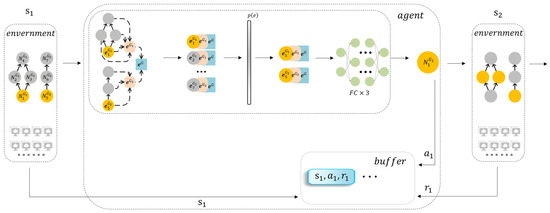
Figure 4. Scheduling process.

Firstly, the agent will observe the environment state, $s_1$, including DAGs and cluster resources, extracting features, $N_n^{G_m}=({\mathit{e}}_n^{G_m},{\mathit{e}}^{G_m},{\mathit{e}}^G)$, as shown in Equations (9)–(11). These features of $N_n^{G_m}$ are filtered in Equation (12) to ensure that only $N_1^{G_1},N_5^{G_2}$ are waiting to be selected. Then, the features of $N_1^{G_1},N_5^{G_2}$ are sent into the policy network to calculate the node probability, $p\left(N_n^{G_m}\right)$. Meanwhile, noise is introduced to increase the randomness. The model will provide a preference to choose $\underset{N_n^{G_m}}{\mathrm{argmax}}\left(p\left(N_n^{G_m}\right)\right)$, assuming that $N_1^{G_1}$ is selected as $\mathit{n}\mathit{o}\mathit{d}\mathit{e}$. Similarly, $\mathit{p}\mathit{a}\mathit{r}\mathit{a}\mathit{l}$ is calculated in the same way. This being the case, $a_1=[\mathit{n}\mathit{o}\mathit{d}\mathit{e},\mathit{p}\mathit{a}\mathit{r}\mathit{a}\mathit{l}]$ is ensured. After $N_1^{G_1}$ is executed, the state, $s_1$, action, $a_1$, and reward, $r_1$, are stored in the buffer. The $r_1$ is obtained by $druation\_time$. The state transfers from $s_1$ to $s_2$ and the action space transfers from $(N_1^{G_1},N_5^{G_2})$ to ${(N}_2^{G_1},N_3^{G_1},N_5^{G_2})$. The agent repeats the above process and selects action $a_t$ until all DAGs have been executed.

Assume that the action trace in the buffer is $(a_1=N_1^{G_1},a_2=N_5^{G_2},a_3=N_2^{G_1},a_4=N_3^{G_1},a_5=N_4^{G_1},a_6=N_6^{G_2},a_7=N_7^{G_2})$. The model will then be optimized with APER by this trace in Figure 5. The agent calculates $R_t$ as shown in Equation (14) and the advantage, $Ad{v}_t$, as shown in Equation (15) for $a_t$. The experience with high $Ad{v}_t$ will be selected according to the sorted $Ad{v}_t$, choosing three experiences, as in Equation (16), and assuming to use $a_1,a_5,a_6$. The agent recalculates the action probability, $p^{\prime }\left(\mathrm{t}\right)$, for the three experiences and then calculates the expected reward, $E\left(r\right)={\sum }_t{p}^{\prime }\left(\mathrm{t}\right)\times Ad{v}_{\mathrm{t}}$. At this time, the $sr$ probability is calculated in addition to the $\mathit{n}\mathit{o}\mathit{d}\mathit{e}$ probability and $\mathit{p}\mathit{a}\mathit{r}\mathit{a}\mathit{l}$ probability. The $sr$ with the highest frequency is affirmed as the sample rate of the next episode, as in Equation (13). Finally, the model is updated by Equation (17) and Equation (18) only if $E\left(r\right)$ is greater than $sum(R_t$) of the corresponding $a_t$. At this point, the first episode is completed.

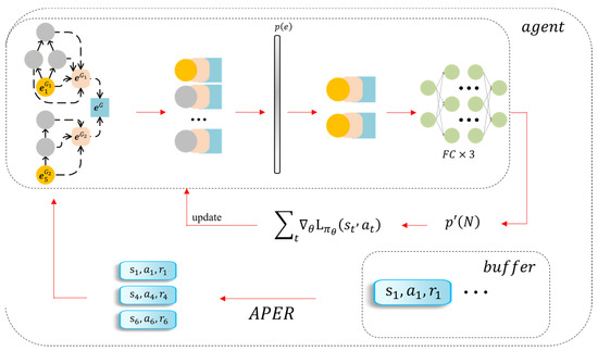
Figure 5. Training process.

In the first episode the agent randomly chooses nodes and the number of experiences. During the rest of the training the agent will utilize trial and error, and learning how to choose actions will increase the rewards in the process. The APER algorithm accelerates learning by prioritizing high $Ad{v}_t$ experience and guarantees performance by gradually adding experience until all traces are learned. This is a simulation of the human learning process.

5. Experiments

5.1. Experiment Settings

Dataset. In this paper, three types of datasets, Tpc h [65], Alibaba cluster data [66] (alidata), and scientific workflows [67], are used for conducting random arrival task scheduling tests. Table 2 shows part of the dataset information. In addition, this paper randomly selects some tasks in order to form a mixed dataset to further enhance the diversity of scheduling scenarios. Experiments show that the scheme in this paper can bring better performance improvements in multiple scenarios.

Table 2. Datasets in this paper.

Dataset	Amount		Sample Amount	Average Arrival Time
Tpc-h	Twenty-two queries are generated under 7 data scales of 2 G, 5 G, 10 G, 20 G, 50 G, 80 G, and 100 G		100	25 s
alidata	Two million from real cluster running data		1000	25 s
Scientific workflows	Scientific Workflow	Number of Nodes	20	50 s
	CyberShake	30, 50, 100, 1000
	Epigenomics	24, 47, 100, 997
	Inspiral	30, 50, 100, 1000
	Montage	25, 50, 100, 1000
	Sipht	29, 58, 97, 968
	Floodplain	7
	HEFT	10
Mixed	1000. 32% from Tpc-h, 64% from alidata, and 4% from scientific workflow		1000	50 s

The model is trained offline by a simulator [10] that can access profiling information from a real Spark cluster, such as JCT and DAG structure. This paper simulates the Poisson process of job arrival, assuming average arrival times of 25 s and 50 s, randomly sampling tasks, and repeating 10 times when using these datasets for testing. This paper treats the scientific workflows as a dataset with 22 DAGs. Decima is used as the comparison algorithm in this paper. It uses a GNN and RL for scheduling decisions and performs well in single scene; however, it has invalid scheduling action and does not have PER.

5.2. Use Different Datasets

Figure 6 shows the JCT of the proposed model and Decima randomly tested on the alidata (a), scientific workflows (b), and Tpc-h (c) 10 times. The ordinate represents JCT, where it being lower indicates better performance. Both of the models are trained using Tpc-h. The model with APER has a steady and huge improvement in alidata. Additionally, the performance is better in most cases when using scientific workflows; however, the performance is worse on Tpc-h in most cases.

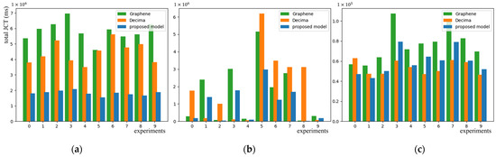
Figure 6. JCT on alidata (a), scientific workflows (b), and Tpc-h (c) using the proposed model, Decima, and Graphene.

The reason why the proposed model works well on alidata is due to it being from a real cluster scheduling trace. Its tasks have stronger diversity and a larger number. Diversity helps the model capture task features more comprehensively. The large number benefits more trial and error of the model and enhances generalization. In contrast, Tpc-h only has 154 pieces of data, and the number of DAG nodes generally ranges from 2 to 18. It is from 2 to 100 in alidata. When good results are achieved on alidata, the model has been “overfitted” on Tpc-h. This paper argues that this is the reason why APER performs worse on Tpc-h.

There are large fluctuations for the two algorithms in scientific workflows. This is because they have fewer pieces of data but larger differences between DAGs. For example, in the same batch of DAGs some DAGs have a small number of stages and high parallelism; some DAGs have major runtimes concentrated in a few stages; and some DAGs have an extremely large number of nodes. However, the performance of the proposed model is still better. Figure 7 and Figure 8 show the variance of all nodes’ JCT and the variance sum of all DAGs’ JCT in Tpc-h and scientific workflows. The variance is calculated using the running time. The differences within the two datasets are shown.

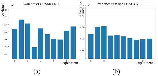
Figure 7. The variance in JCT in Tpc-h.

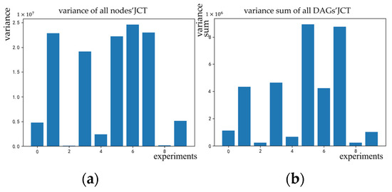
Figure 8. The variance in JCT in scientific workflows.

In the zeroth, second, fourth, and eighth experiments the variance in the two graphs is low, denoting that the execution times of all of the nodes are relatively close. At this time, the four scheduling strategies can achieve better performance. The variances in the third and seventh experiments are relatively large, denoting that the difference in the task execution times between nodes in a single DAG is high. In addition, the execution times of all of the DAG nodes are also different. Compared with Decima, this paper model is more suitable for highly random scheduling processes. In the sixth experiment the overall variance is extremely high, but the sum of the variances of the DAG is low, showing that the difference in the execution times of nodes within a single DAG is low but the difference between each DAG is extremely large. For example, the number of sampled scientific workflow nodes is around 1000 or below 50. The model is difficult to adapt to drastic changes with fewer DAGs, but it performs better in mixed data, as shown in Figure 9. Compared with Decima, this model still has certain advantages in many scenarios.

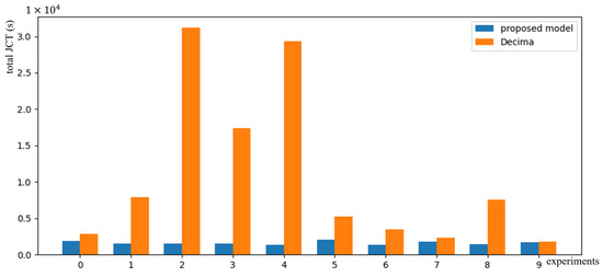
Figure 9. Result on the mixed dataset of 1000 DAGs.

Considering the characteristics of three datasets, the mixed dataset consists of 32% Tpc-h, 64% alidata, and 4% scientific workflows, which is then tested 10 times. The Figure 9 shows the performance comparison plots of the proposed model and Decima on the mixed dataset tested 10 times. It is observed that the proposed model generally outperforms the contrastive models. Table 3 shows the JCT of 10 experiments, showing that this model’s JCT is better than Decima on the mixed dataset, with an average advantage of around 37%, with higher $R$ and shorter task completion times. The fluctuation in the third, fourth, and fifth tests is because the sampled DAG variance is too high.

Table 3. JCT(s) on the mixed dataset.

	1	2	3	4	5	6	7	8	9	10	Total	Average
The proposed model	1864.8	1560.6	1505.3	1556.0	1377.1	2014.3	1313.9	1768.3	1430.8	1724.6	16,115.7	1611.6
Decima	2854.5	7879.6	31,178.6	17,337.5	29,293.5	5221.1	3498.1	2281.9	7574.0	1748.7	108,867.4	10,886.7
Relative advantage This model/Decima	65.33%	19.81%	4.83%	8.97%	4.70%	38.58%	37.56%	77.49%	18.89%	98.62%	14.80%	37.48%

5.3. Comparison of Different Algorithms

In this paper’s experiments, some common algorithms and state-of-the-art algorithms are used for comparison:

(1)

Decima with idle slots [20]. Based on Decima, the JCT can be reduced by delaying the running of some tasks for a period by intentionally inserting idle time slots for relatively large tasks.

(2)

GARLSched [68]. A reinforcement learning scheduling algorithm combined with generative adversarial networks. It uses an optimal policy in the expert database to guide agents to learn in large-scale dynamic scheduling problems while using a discriminator network based on task embedding to improve and stabilize the training process. This is an independent task scheduling algorithm.

(3)

Graphene [69]. A classic task heuristic scheduler based on DAGs and heterogeneous resources. It improves cluster performance by discovering potential parallelism in DAGs.

Table 4 shows the average JCT and relative performance of the proposed model and the comparison model when using Alibaba cluster data. These figures are calculated through comparison with Decima. “/” indicates that the comparison algorithm did not perform, and the original algorithms are also no test results. The average JCT is calculated by Equation (4).

Table 4. Average JCT of different algorithms on Tpc-h and alidata.

Algorithm	Proposed Model	Decima	Decima with Idle Slots	GARLSched	Graphene
Average JCT on Tpc-h	58.93	53.57	/	/	76.61
Average JCT on alidata	182.04	444.01	381.85	261.69	586.09

When using APER, the average JCT of each DAG on alidata is only 41% of Decima, which is better than other comparison algorithms. This paper argues that the reason for the better results of Decima is that Tpc-h is used to train and test simultaneously. This is corroborated by the JCT of Decima over the proposed model on Tpc-h, which is consistent with the Figure 6. Because alidata are from real cluster traces, it can be considered that this model is more suitable for real scheduling scenarios.

5.4. Ablation Experiment

APER can not only enhance the robustness when a large amount of experience is used, making it suitable for more application scenarios, but it can also help models converge if using a small amount of good experience. Figure 10 shows convergence curves, in which a is when using APER and b is without using APER. The loss is calculated according to Equation (10), and it will increase until convergence. Although both graphs converge at around 1000 episodes, this is because $w_e$ does not drop to a fixed value until the 1000th episode and the impact of $En{t}_{{\pi }_{\theta }}\left(a_t\right)$ is huge in the early stage. Starting from the 400th episode, the model is stable to use for all experiments. This is also why the convergence curve has smaller and smaller fluctuations before the 400th episode but steadily rises after that. This paper believes that steady convergence instead of violent fluctuation is one of the reasons why the model can achieve better performance in the early stage, because the model can perform scheduling decisions under a relatively stable policy.

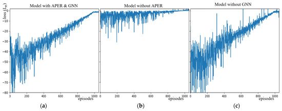
Figure 10. Convergence curves. (a) APER and GNN; (b) without APER; and (c) without GNN.

The paper also tests the role of a GNN. Figure 10c shows the convergence curve of the model without a GNN. The loss curve is similar to Figure 10a, which shows the effectiveness of APER; however, it converges more slowly. It is shown that loss fluctuates greatly without a GNN. This is because a GNN is used to extract dependencies between nodes in a DAG. It aggregates the information of each node and its successors, which is equivalent to pre-calculating the time from this node to the end of a DAG for each node. This way of predicting the completion time of each DAG measures the value of each schedulable node from a global perspective and makes the model more inclined to take scheduling actions that can reduce the total task completion time. The model without GNN can calculate scheduling actions only based on the information of schedulable nodes and cannot consider the global perspective. The model will prefer to select nodes with shorter execution times rather than nodes with shorter expected DAG completion times. This may lead to a longer JCT, thus making the loss more volatile. Finally, this paper selected the stabilized proposed model and the model without a GNN for ten instances of testing on the mixed dataset. This is shown in Figure 11, where orange is the proposed model and blue is the model without a GNN. As mentioned above, the model without a GNN performs worse.

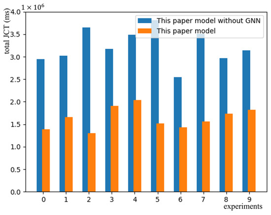
Figure 11. Impact of a GNN on JCT.

6. Discussion and Conclusions

Task scheduling in cloud environments has been a research hotspot. This paper designs a cloud platform task scheduling model based on APER, which is used to improve a platform’s adaptability to complex, dynamic, and multiscenario scheduling tasks. The model can directly optimize a scheduling strategy by interacting with a cloud platform, as well as by gradually expanding from specific experience to general experience, to ensure that the model can achieve better results in complex environments. The experimental results show that the proposed model not only has a more robust performance in random scheduling environments in various scenarios but also accelerates convergence to a certain extent. This demonstrates the effectiveness of the scheduling framework and APER.

The proposed algorithm still has some shortcomings and optimization directions: (1) Pre-emptive scheduling. In real cloud platforms it is often necessary to consider urgent tasks. It is possible to consider task priority while calculating scheduling actions or using MARL. (2) Add performance metrics. The performance metrics of the proposed model are relatively simple, and others, such as the loading time of hardware resources, throughput, waiting time, etc., can be used at the same time.

References

- Grandl, R.; Ananthanarayanan, G.; Kandula, S.; Rao, S.; Akella, A. Multi-Resource Packing for Cluster Schedulers. SIGCOMM Comput. Commun. Rev. 2014, 44, 455–466. [Google Scholar] [CrossRef]
- Li, F.; Hu, B. DeepJS: Job Scheduling Based on Deep Reinforcement Learning in Cloud Data Center. In Proceedings of the 4th International Conference on Big Data and Computing, NewYork, NY, USA, 10–12 May 2019; pp. 48–53. [Google Scholar] [CrossRef]
- Sahu, D.P.; Singh, K.; Prakash, S. Maximizing Availability and Minimizing Markesan for Task Scheduling in Grid Computing Using NSGA II. In Proceedings of the Second International Conference on Computer and Communication Technologies, New Delhi, India, 24–26 July 2015; pp. 219–224. [Google Scholar] [CrossRef]
- Keshanchi, B.; Souri, A.; Navimipour, N.J. An improved genetic algorithm for task scheduling in the cloud environments using the priority queues: Formal verification, simulation, and statistical testing. J. Syst. Softw. 2017, 124, 1–21. [Google Scholar] [CrossRef]
- Chen, L.; Liu, S.H.; Li, B.C.; Li, B. Scheduling Jobs across Geo-Distributed Datacenters with Max-Min Fairness. IEEE Trans. Netw. Sci. Eng. 2019, 6, 488–500. [Google Scholar] [CrossRef]
- Al-Zoubi, H. Efficient Task Scheduling for Applications on Clouds. In Proceedings of the 2019 6th IEEE International Conference on Cyber Security and Cloud Computing (CSCloud)/2019 5th IEEE International Conference on Edge Computing and Scalable Cloud (EdgeCom), Paris, France, 21–23 June 2019; pp. 10–13. [Google Scholar] [CrossRef]
- Kumar, A.M.S.; Parthiban, K.; Shankar, S.S. An efficient task scheduling in a cloud computing environment using hybrid Genetic Algorithm—Particle Swarm Optimization (GA-PSO) algorithm. In Proceedings of the 2019 International Conference on Intelligent Sustainable Systems, Tokyo, Japan, 21–22 February 2019; pp. 29–34. [Google Scholar] [CrossRef]
- Faragardi, H.R.; Sedghpour, M.R.S.; Fazliahmadi, S.; Fahringer, T.; Rasouli, N. GRP-HEFT: A Budget-Constrained Resource Provisioning Scheme for Workflow Scheduling in IaaS Clouds. IEEE Trans. Parallel Distrib. Syst. 2020, 31, 1239–1254. [Google Scholar] [CrossRef]
- Kumar, K.R.P.; Kousalya, K. Amelioration of task scheduling in cloud computing using crow search algorithm. Neural Comput. Appl. 2020, 32, 5901–5907. [Google Scholar] [CrossRef]
- Mao, H.; Schwarzkopf, M.; Venkatakrishnan, S.B.; Meng, Z.; Alizadeh, M. Learning scheduling algorithms for data processing clusters. In Proceedings of the ACM Special Interest Group on Data Communication, Beijing, China, 19–23 August 2019; pp. 270–288. [Google Scholar] [CrossRef]
- Zade, M.H.; Mansouri, N.; Javidi, M.M. A two-stage scheduler based on New Caledonian Crow Learning Algorithm and reinforcement learning strategy for cloud environment. J. Netw. Comput. Appl. 2022, 202, 103–385. [Google Scholar] [CrossRef]
- Huang, B.; Xia, W.; Zhang, Y.; Zhang, J.; Zou, Q.; Yan, F.; Shen, L. A task assignment algorithm based on particle swarm optimization and simulated annealing in Ad-hoc mobile cloud. In Proceedings of the 9th International Conference on Wireless Communications and Signal Processing (WCSP), Nanjing, China, 11–13 October 2017; pp. 1–6. [Google Scholar] [CrossRef]
- Wu, F.; Wu, Q.; Tan, Y.; Li, R.; Wang, W. PCP-B2: Partial critical path budget balanced scheduling algorithms for scientific workflow applications. Future Gener. Comput. Syst. 2016, 60, 22–34. [Google Scholar] [CrossRef]
- Zhou, X.M.; Zhang, G.X.; Sun, J.; Zhou, J.L.; Wei, T.Q.; Hu, S.Y. Minimizing cost and makespan for workflow scheduling in cloud using fuzzy dominance sort based HEFT. Future Gener. Comput. Syst. 2019, 93, 278–289. [Google Scholar] [CrossRef]
- Xing, L.; Zhang, M.; Li, H.; Gong, M.; Yang, J.; Wang, K. Local search driven periodic scheduling for workflows with random task runtime in clouds. Comput. Ind. Eng. 2022, 168, 14. [Google Scholar] [CrossRef]
- Peng, Z.P.; Cui, D.L.; Zuo, J.L.; Li, Q.R.; Xu, B.; Lin, W.W. Random task scheduling scheme based on reinforcement learning in cloud computing. Clust. Comput. J. Netw. Softw. Tools Appl. 2015, 18, 1595–1607. [Google Scholar] [CrossRef]
- Ran, L.; Shi, X.; Shang, M. SLAs-Aware Online Task Scheduling Based on Deep Reinforcement Learning Method in Cloud Environment. In Proceedings of the IEEE 21st International Conference on High Performance Computing and Communications; IEEE 17th International Conference on Smart City; IEEE 5th International Conference on Data Science and Systems (HPCC/SmartCity/DSS), Zhangjiajie, China, 10–12 August 2019; pp. 1518–1525. [Google Scholar] [CrossRef]
- Qin, Y.; Wang, H.; Yi, S.; Li, X.; Zhai, L. An Energy-Aware Scheduling Algorithm for Budget-Constrained Scientific Workflows Based on Multi-Objective Reinforcement Learning. J. Supercomput. 2020, 76, 455–480. [Google Scholar] [CrossRef]
- Wang, J.J.; Wang, L. A Cooperative Memetic Algorithm With Learning-Based Agent for Energy-Aware Distributed Hybrid Flow-Shop Scheduling. IEEE Trans. Evol. Comput. 2022, 26, 461–475. [Google Scholar] [CrossRef]
- Duan Yubin, W.J. Improving Learning-Based DAG Scheduling by Inserting Deliberate Idle Slots. IEEE Netw. Mag. Glob. Internetw. 2021, 35, 133–139. [Google Scholar] [CrossRef]
- Sutton, R.S.; Barto, A.G. Reinforcement Learning: An Introduction; MIT Press: Cambridge, MA, USA, 1998; p. 342. [Google Scholar] [CrossRef]
- Yang, T.; Tang, H.; Bai, C.; Liu, J.; Hao, J.; Meng, Z.; Liu, P. Exploration in Deep Reinforcement Learning: A Comprehensive Survey. Inf. Fusion 2021, 85, 1–22. [Google Scholar] [CrossRef]
- Rjoub, G.; Bentahar, J.; Wahab, O.A.; Bataineh, A. Deep Smart Scheduling: A Deep Learning Approach for Automated Big Data Scheduling Over the Cloud. In Proceedings of the 2019 7th International Conference on Future Internet of Things and Cloud (FiCloud), Istanbul, Turkey, 26–28 August 2019; pp. 189–196. [Google Scholar] [CrossRef]
- Wei, Y.; Pan, L.; Liu, S.; Wu, L.; Meng, X. DRL-Scheduling: An Intelligent QoS-Aware Job Scheduling Framework for Applications in Clouds. IEEE Access 2018, 6, 55112–55125. [Google Scholar] [CrossRef]
- Yi, D.; Zhou, X.; Wen, Y.; Tan, R. Toward Efficient Compute-Intensive Job Allocation for Green Data Centers: A Deep Reinforcement Learning Approach. In Proceedings of the 2019 IEEE 39th International Conference on Distributed Computing Systems (ICDCS), Dallas, TX, USA, 7–10 July 2019; pp. 634–644. [Google Scholar] [CrossRef]
- Wang, L.; Huang, P.; Wang, K.; Zhang, G.; Zhang, L.; Aslam, N.; Yang, K. RL-Based User Association and Resource Allocation for Multi-UAV enabled MEC. In Proceedings of the 2019 15th International Wireless Communications & Mobile Computing Conference (IWCMC), Tangier, Morocco, 24–28 June 2019; pp. 741–746. [Google Scholar] [CrossRef]
- Chen, X.; Zhang, H.; Wu, C.; Mao, S.; Ji, Y.; Bennis, M. Performance Optimization in Mobile-Edge Computing via Deep Reinforcement Learning. In Proceedings of the 2018 IEEE 88th Vehicular Technology Conference (VTC-Fall), Chicago, IL, USA, 27–30 August 2018; pp. 1–6. [Google Scholar] [CrossRef]
- Cheng, F.; Huang, Y.; Tanpure, B.; Sawalani, P.; Cheng, L.; Liu, C. Cost-aware job scheduling for cloud instances using deep reinforcement learning. Clust. Comput. 2022, 25, 619–631. [Google Scholar] [CrossRef]
- Yan, J.; Huang, Y.; Gupta, A.; Liu, C.; Li, J.; Cheng, L. Energy-aware systems for real-time job scheduling in cloud data centers: A deep reinforcement learning approach. Comput. Electr. Eng. 2022, 99, 10. [Google Scholar] [CrossRef]
- Li, T.; Xu, Z.; Tang, J.; Wang, Y. Model-free control for distributed stream data processing using deep reinforcement learning. Proc. VLDB Endow. 2018, 11, 705–718. [Google Scholar] [CrossRef]
- Mao, H.; Alizadeh, M.; Menache, I.; Kandula, S. Resource Management with Deep Reinforcement Learning. In Proceedings of the 15th ACM Workshop on Hot Topics in Networks, Atlanta, GA, USA, 9–10 November 2016; pp. 50–56. [Google Scholar]
- Lee, H.; Lee, J.; Yeom, I.; Woo, H. Panda: Reinforcement Learning-Based Priority Assignment for Multi-Processor Real-Time Scheduling. IEEE Access 2020, 8, 185570–185583. [Google Scholar] [CrossRef]
- Di Zhang, D.D.; He, Y.; Bao, F.S.; Xie, B. RLScheduler: Learn to Schedule Batch Jobs Using Deep Reinforcement Learning. In Proceedings of the International Conference for High Performance Computing, Networking, Storage and Analysis, Atlanta, GA, USA, 9–19 November 2020; pp. 1–15. [Google Scholar] [CrossRef]
- Liang, S.; Yang, Z.; Jin, F.; Chen, Y. Data centers job scheduling with deep reinforcement learning. In Proceedings of the Advances in Knowledge Discovery and Data Mining: 24th Pacific-Asia Conference, PAKDD 2020, Singapore, 11–14 May 2020; pp. 906–917. [Google Scholar] [CrossRef]
- Liu, Q.; Shi, L.; Sun, L.; Li, J.; Ding, M.; Shu, F. Path Planning for UAV-Mounted Mobile Edge Computing with Deep Reinforcement Learning. IEEE Trans. Veh. Technol. 2020, 69, 5723–5728. [Google Scholar] [CrossRef]
- Wang, L.; Weng, Q.; Wang, W.; Chen, C.; Li, B. Metis: Learning to Schedule Long-Running Applications in Shared Container Clusters at Scale. In Proceedings of the SC20: International Conference for High Performance Computing, Networking, Storage and Analysis, Atlanta, GA, USA, 9–19 November 2020; pp. 1–17. [Google Scholar] [CrossRef]
- Mitsis, G.; Tsiropoulou, E.E.; Papavassiliou, S. Price and Risk Awareness for Data Offloading Decision-Making in Edge Computing Systems. IEEE Syst. J. 2022, 16, 6546–6557. [Google Scholar] [CrossRef]
- Souri, A.; Zhao, Y.; Gao, M.; Mohammadian, A.; Shen, J.; Al-Masri, E. A Trust-Aware and Authentication-Based Collaborative Method for Resource Management of Cloud-Edge Computing in Social Internet of Things. IEEE Trans. Comput. Soc. Syst. 2023, 1–10. [Google Scholar] [CrossRef]
- Long, X.J.; Zhang, J.T.; Qi, X.; Xu, W.L.; Jin, T.G.; Zhou, K. A self-learning artificial bee colony algorithm based on reinforcement learning for a flexible job-shop scheduling problem. Concurr. Comput. Pract. Exp. 2022, 34, e6658. [Google Scholar] [CrossRef]
- Paliwal, A.S.; Gimeno, F.; Nair, V.; Li, Y.; Lubin, M.; Kohli, P.; Vinyals, O. Reinforced Genetic Algorithm Learning for Optimizing Computation Graphs. In Proceedings of the 2020 International Conference on Learning Representations, Addis Ababa, Ethiopia, 11 March 2020; pp. 1–24. [Google Scholar]
- Gao, Y.; Chen, L.; Li, B. Spotlight: Optimizing Device Placement for Training Deep Neural Networks. In Proceedings of the 35th International Conference on Machine Learning, Proceedings of Machine Learning Research, Stockholm, Sweden, 10–15 July 2018; pp. 1676–1684. [Google Scholar]
- Chen, X.; Tian, Y. Learning to perform local rewriting for combinatorial optimization. In Proceedings of the 33rd International Conference on Neural Information Processing Systems, Vancouver, BC, Canada, 8–14 December 2019; Curran Associates: New York, NY, USA; p. 564. [Google Scholar]
- Bao, Y.; Peng, Y.; Wu, C. Deep Learning-Based Job Placement in Distributed Machine Learning Clusters With Heterogeneous Workloads. IEEE/ACM Trans. Netw. 2022, 1–14. [Google Scholar] [CrossRef]
- Lee, H.; Cho, S.; Jang, Y.; Lee, J.; Woo, H. A Global DAG Task Scheduler Using Deep Reinforcement Learning and Graph Convolution Network. IEEE Access 2021, 9, 158548–158561. [Google Scholar] [CrossRef]
- Hu, Z.; Tu, J.; Li, B. Spear: Optimized Dependency-Aware Task Scheduling with Deep Reinforcement Learning. In Proceedings of the 2019 IEEE 39th International Conference on Distributed Computing Systems (ICDCS), Dallas, TX, USA, 7–10 July 2019; pp. 2037–2046. [Google Scholar] [CrossRef]
- Gao, Y.; Chen, L.; Li, B. Post: Device placement with cross-entropy minimization and proximal policy optimization. In Proceedings of the 32nd International Conference on Neural Information Processing Systems, Montréal, QC, Canada, 3–8 December 2018; pp. 9993–10002. [Google Scholar]
- Mirhoseini, A.; Pham, H.; Le, Q.V.; Steiner, B.; Larsen, R.; Zhou, Y.; Kumar, N.; Norouzi, M.; Bengio, S.; Dean, J. Device placement optimization with reinforcement learning. In Proceedings of the 34th International Conference on Machine Learning—Volume 70, Sydney, NSW, Australia, 6–11 August 2017; pp. 2430–2439. [Google Scholar]
- Zhu, J.; Li, Q.; Ying, S. SAAS parallel task scheduling based on cloud service flow load algorithm. Comput. Commun. 2022, 182, 170–183. [Google Scholar] [CrossRef]
- Kipf, T.; Welling, M. Semi-Supervised Classification with Graph Convolutional Networks. In Proceedings of the International Conference on Learning Representations, Toulon, France, 24–26 April 2017. [Google Scholar] [CrossRef]
- Zhang, C.; Song, W.; Cao, Z.; Zhang, J.; Tan, P.S.; Xu, C. Learning to Dispatch for Job Shop Scheduling via Deep Reinforcement Learning. Adv. Neural Inf. Process. Syst. 2020, 33, 1621–1632. [Google Scholar]
- Sun, P.; Guo, Z.; Wang, J.; Li, J.; Lan, J.; Hu, Y. DeepWeave: Accelerating job completion time with deep reinforcement learning-based coflow scheduling. In Proceedings of the Twenty-Ninth International Joint Conference on Artificial Intelligence, Yokohama, Japan, 11–17 July 2020; p. 458. [Google Scholar]
- Grinsztajn, N.; Beaumont, O.; Jeannot, E.; Preux, P.; Soc, I.C. READYS: A Reinforcement Learning Based Strategy for Heterogeneous Dynamic Scheduling. In Proceedings of the IEEE International Conference on Cluster Computing (Cluster), Electr Network, Portland, OR, USA, 7–10 September 2021; pp. 70–81. [Google Scholar] [CrossRef]
- Wang, C.; Wu, Y.; Vuong, Q.; Ross, K. Striving for Simplicity and Performance in Off-Policy DRL: Output Normalization and Non-Uniform Sampling. In Proceedings of the 37th International Conference on Machine Learning, Vienna, Austria, 13–18 July 2020; p. 11. [Google Scholar] [CrossRef]
- Atherton, L.A.; Dupret, D.; Mellor, J.R. Memory trace replay: The shaping of memory consolidation by neuromodulation. Trends Neurosci. 2015, 38, 560–570. [Google Scholar] [CrossRef]
- Schaul, T.; Quan, J.; Antonoglou, I.; Silver, D. Prioritized Experience Replay. In Proceedings of the 4th International Conference on Learning Representations, San Juan, Puerto Rico, 2–4 May 2016. [Google Scholar] [CrossRef]
- Kumar, A.; Gupta, A.; Levine, S. DisCor: Corrective Feedback in Reinforcement Learning via Distribution Correction. In Proceedings of the Conference and Workshop on Neural Information Processing Systems, Virtual, 6–12 December 2020. [Google Scholar] [CrossRef]
- Liu, X.-H.; Xue, Z.; Pang, J.-C.; Jiang, S.; Xu, F.; Yu, Y. Regret Minimization Experience Replay in Off-Policy Reinforcement Learning. In Proceedings of the Advances in Neural Information Processing Systems 34: Annual Conference on Neural Information Processing Systems 2021, Virtual, 6–14 December 2021; pp. 17604–17615. [Google Scholar] [CrossRef]
- Bengio, Y.; Louradour, J.; Collobert, R.; Weston, J. Curriculum learning. Int. Conf. Mach. Learn. 2009, 139, 41–48. [Google Scholar] [CrossRef]
- Bondy, J.A.; Murty, U.S.R. Graph Theory with Applications. Soc. Ind. Appl. Math. 1976, 21, 429. [Google Scholar] [CrossRef]
- Lin, L.J. Self-Improving Reactive Agents Based on Reinforcement Learning, Planning and Teaching. Mach. Learn. 1992, 8, 293–321. [Google Scholar] [CrossRef]
- Chen, H.; Zhu, X.; Liu, G.; Pedrycz, W. Uncertainty-Aware Online Scheduling for Real-Time Workflows in Cloud Service Environment. IEEE Trans. Serv. Comput. 2021, 14, 1167–1178. [Google Scholar] [CrossRef]
- Gari, Y.; Monge, D.A.; Mateos, C. A Q-learning approach for the autoscaling of scientific workflows in the Cloud. Future Gener. Comput. Syst. Int. J. Escience 2022, 127, 168–180. [Google Scholar] [CrossRef]
- Hasselt, H.V.; Guez, A.; Silver, D. Deep Reinforcement Learning with Double Q-Learning. In Proceedings of the Thirtieth AAAI Conference on Artificial Intelligence, Phoenix, AZ, USA, 12–17 February 2016; pp. 2094–2100. [Google Scholar] [CrossRef]
- Wu, L.J.; Tian, F.; Xia, Y.; Fan, Y.; Qin, T.; Lai, J.H.; Liu, T.Y. Learning to Teach with Dynamic Loss Functions. In Proceedings of the 32nd International Conference on Neural Information Processing Systems, Red Hook, NY, USA, 3–8 December 2018; pp. 6467–6478. [Google Scholar] [CrossRef]
- TPC-H. The TPC-H Benchmarks. Available online: https://www.tpc.org/tpch/ (accessed on 10 April 2022).
- Guo, J.; Chang, Z.; Wang, S.; Ding, H.; Feng, Y.; Mao, L.; Bao, Y. Who limits the resource efficiency of my datacenter: An analysis of Alibaba datacenter traces. In Proceedings of the 2019 IEEE/ACM 27th International Symposium on Quality of Service (IWQoS), Phoenix, AZ, USA; 2019; pp. 1–10. [Google Scholar] [CrossRef]
- Bharathi, S.; Chervenak, A.; Deelman, E.; Mehta, G.; Su, M.H.; Vahi, K. Characterization of scientific workflows. In Proceedings of the Third Workshop on Workflows in Support of Large-Scale Science, Austin, TX, USA, 17 November 2008; pp. 1–10. [Google Scholar] [CrossRef]
- Li, J.B.; Zhang, X.J.; Wei, J.; Ji, Z.Y.; Wei, Z. GARLSched: Generative adversarial deep reinforcement learning task scheduling optimization for large-scale high performance computing systems. Future Gener. Comput. Syst. Int. J. Escience 2022, 135, 259–269. [Google Scholar] [CrossRef]
- Grandl, R.; Kandula, S.; Rao, S.; Akella, A.; Kulkarni, J. Graphene: Packing and Dependency-Aware Scheduling for Data-Parallel Clusters. In Proceedings of the 12th USENIX conference on Operating Systems Design and Implementation, Savannah, GA, USA; 2016; pp. 81–97. [Google Scholar] [CrossRef]
Disclaimer/Publisher’s Note: The statements, opinions and data contained in all publications are solely those of the individual author(s) and contributor(s) and not of MDPI and/or the editor(s). MDPI and/or the editor(s) disclaim responsibility for any injury to people or property resulting from any ideas, methods, instructions or products referred to in the content. |
© 2023 by the authors. Licensee MDPI, Basel, Switzerland. This article is an open access article distributed under the terms and conditions of the Creative Commons Attribution (CC BY) license (https://creativecommons.org/licenses/by/4.0/).