Abstract
During the last decade, field oriented control has often been implemented with space vector modulation due to its inherent advantages over other modulation techniques. On the other hand, direct flux control is a method that estimates the rotor electrical position of synchronous machines (e.g., permanent magnet synchronous motors) using only voltage measurements. In simple terms, direct flux control replaces position sensors by measuring the voltage difference between the star point of the synchronous machine and an artificial star point at particular instants during the switching pattern. Indeed, previous work dealt with direct flux control resorting exclusively to sinusoidal pulse width modulation and mostly in open-loop speed control schemes. This paper aims to present a space vector modulation-based direct flux control measurement sequence that can be used directly with field oriented control to perform sensorless speed control of synchronous machines. In contrast with previous publications, the direct flux control measurement sequence proposed in this paper not only extracts the direct flux control flux linkage signals with the same offset level but also obtains the phase currents needed for field oriented control without current ripple. In simple terms, the proposed direct flux control measurement sequence based on space vector modulation can be used with field oriented control to perform sensorless closed-loop speed control of synchronous machines. The sensorless speed control with the space vector modulation-based direct flux control sequence is validated for high speeds (80% of the nominal speed) and low speeds (6% of the nominal speed) using a high-fidelity four-pole synchronous machine’s simulation model implemented in ANSYS Simplorer and Maxwell.
1. Introduction
Among the different types of electrical motors, synchronous motors (e.g., permanent magnet synchronous motors (PMSMs)) are chosen most of the time for high-performance variable speed drive systems [1,2,3]. The reason for this are the superior characteristics of synchronous motors over their DC and induction counterparts such as higher efficiency, higher power density, and higher reliability [3,4]. In addition, synchronous motors exhibit a higher torque to inertia ratio than DC and induction motors that ultimately leads to small ramp-up times and to very high dynamics [5]. However, in order to exploit at their maximum all the capabilities of synchronous motors, field oriented control algorithms are needed to command these types of motors [6,7]. As in synchronous motors, torque production is related with the control of the magnitude and orientation of the current vector with respect to the rotor flux; the rotor position which is aligned with the rotor magnetic flux is needed. In fact, the current vector created by the three-phase windings should remain at an optimal electrical angle with respect to the rotor magnetic flux at all speeds [8]. Only under these conditions will the best torque/current ratio or the maximum torque per unit of current be achieved [9]. Obviously, the synchronous motor’s rotor position needed to perform field oriented control can be obtained though physical position sensors such as absolute encoders or resolvers [5,10]. However, these additional sensors demand extra costs and extra cables, and make the synchronous motor’s shaft length larger [11]. The latter two unfortunately reduce the reliability and the power density of the entire drive system. In addition, the cable from position sensor to control unit can be affected by EMI noise due to PWM switching which could deteriorate the field oriented control performance [12]. For this reason, in recent years, a lot of work has been carried in the so-called sensorless control methods. These use the electrical machines directly as sensors to obtain the rotor position [13].
Generally speaking, the sensorless control methods can be divided into two groups: methods for middle- to high-speed operation (i.e., speeds starting at 20% of the nominal speed) and methods for standstill or very low speeds [2,11]. On the one hand, methods for middle- to high-speed operation are normally based in mathematical models of the synchronous motor. Thus, they need the machine’s physical parameters [14]. Examples of methods that belong to this group are open-loop observers, closed-loop observers [15], and adaptative observers [16,17]. On the other hand, the methods for standstill and low-speed operation exploit the machine’s inductance variation, and they do not require the parameters of the machine. These methods exploit the fact that the synchronous motor’s stator self-inductances vary as a function of the rotor position due to the magnetic saliency of the AC machine [2]. Actually, the saliency-based methods are considered still under development [12], and the most important exponents of this group are the high-frequency injection methods [18,19,20]. However, other methods that exploit the saliency of the AC machine exist, and they have been not so extensively studied as the high-frequency injection methods. The latter is the case of the INFORM method [21,22] and the Direct Flux Control (DFC) method [23,24]. Although both methods send pulsating voltage signals to the machine in order to obtain the rotor position, the difference lies in the output signal used for the rotor position estimation. In detail, the INFORM method measures current signals to estimate the rotor position, whereas the DFC method uses voltage signals to perform the same estimation [25]. The first advantage of the DFC method over the INFORM method is that it is easier to process voltage signals than current signals with the aim to estimate the rotor position. The second advantage of the DFC method is that it can estimate the rotor position also at high speeds where the INFORM method and other high frequency injection methods exhibit limitations [26]. Naturally, DFC also exhibits some disdvantages as it requires additional voltage sensors, additional resistances for the artificial star point, and extra cabling to capture the voltage measurements.
The DFC method was developed originally by Strothmann and patented in [27]. Subsequently, Mantala et al. analyzed the DFC method in detail in [28,29,30]. In summary, DFC is a sensorless method that estimates the synchronous motor’s rotor position from the so-called DFC flux linkage signals (u,v,w). The DFC flux linkage signals embody the rotor flux position and they can be obtained from voltage measurements between the star point fo the machine () and an artificial star point (). The latter is made of pure resistive elements which are connected in parallel to the machine (see Figure 1). Furthermore, the voltage measurement between the star points, namely the voltage , must be evaluated at precise intervals within the switching pulse pattern in order to extract the DFC flux linkage signals correctly. On this basis, the first measurement sequence to extract the DFC flux linkage signals was proposed by Strothmann in [27]. Based on this original measurement sequence (see Figure 2), DFC was used in an open-loop speed control structure in [31], and in a speed closed-loop structure with field oriented control in [30,32]. Unfortunately, the problem of the original measurement sequence is that the DFC flux linkage signals are extracted with a different offset level in each phase. Different offsets in each DFC flux linkage signal are more difficult to compensate and, for that matter, the rotor position estimation is affected negatively [33]. On account of this, Mantala derived mathematically a second DFC measurement sequence in [30] based on Sinusoidal Pulse Width Modulation (SPWM). This second measurement sequence solves the offset asymmetry in the extracted DFC flux linkage signals inherent to the original measurement sequence. Afterwards, Grasso et al. in [34,35] tested successfully the second DFC measurement sequence in an experimental setup validating Mantala’s mathematical derivations. On this basis, the second DFC measurement sequence was then implemented within an open-loop speed control structure in [36].
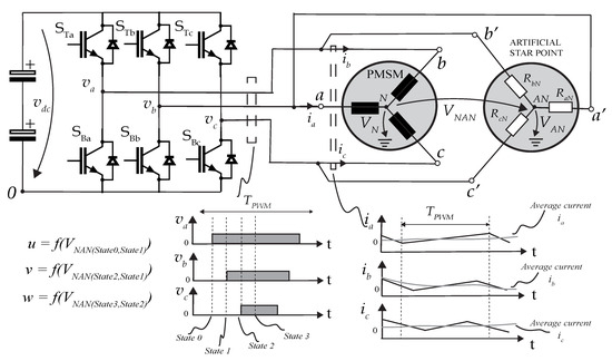
Figure 1.
DFC Flux linkage signals’ measurement scheme.
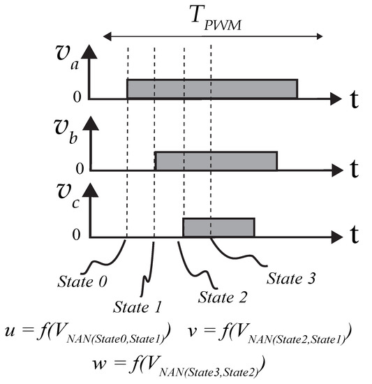
Figure 2.
Original DFC measurement sequence: Inverter’s states for DFC flux linkage measurement.
Furthermore, a DFC measurement sequence meant to be used in conjunction with Space Vector Modulation (SVM) was presented by the authors of this paper in [37]. In addition, the SVM-based DFC measurement sequence was utilized in a speed closed-loop structure with field oriented control in the same reference. To the best of the authors’ knowledge, the SVM-based DFC measurement sequence was used for the first time in a speed closed-loop structure with field oriented control in our previous conference paper. Indeed, this paper comes to expand the work presented in [37] providing three novel aspects. First, a detailed mathematical derivation of the modified DFC measurement sequence that is used it conjunction with SVM is presented. Second, the field oriented control structure that uses the SVM-based DFC measurement sequence is explained in great detail. Last but not least, additional results of the sensorless field oriented control with the SVM-based DFC measurement sequence for low and high speeds that were not previously disclosed are shown. To this end, this paper is organized in six sections. First, Section 2 discusses the derivation of the SVM-based DFC measurement sequence that is compatible with field oriented control. Afterwards, Section 3 covers the speed control structure with field oriented control that uses the proposed DFC measurement sequence. Then, Section 4 describes in detail the high-fidelity simulation model used to validate the sensorless speed control loop with field oriented control and DFC. The high-fidelity model consists of a finite element model (FEM) of a synchronous machine created in ANSYS Maxwell that is coupled with a power electronics circuit implemented in the software ANSYS Simplorer. Subsequently, Section 5 shows and discusses the results obtained for the sensorless speed control with field oriented control and the SVM-based DFC for low and high speeds. Finally, Section 6 presents the main conclusions and outlook.
2. SVM-Based DFC Measurement Sequence
The DFC flux linkage signals are obtained measuring the voltage at particular states during the switching pattern produced by the inverter. Therefore, an external pure resistive circuit connected in star needs to be connected in parallel to the synchronous motor’s machine terminals (see Figure 1). As it is important to avoid the current flow through the additional resistive circuit, the values of the additional resistances (,,) should be much higher than the phase impedances of the synchronous motor. Actually, resistance values between 200 k and 470 k are recommended for the construction of the artificial star point [28]. Furthermore, although field oriented control can be used with any kind of modulation technique, in recent times, SVM is the preferred modulation technique for field oriented control [38]. This is because SVM allows for a bigger amplitude for the voltage space vector that is fed to the motor for the same DC-Link voltage level and the same inverter topology than other techniques such as Sinusoidal Pulse Width Modulation (SPWM) [5]. A second reason is that many SVM algorithms exist whose inputs can receive directly the reference voltage space vector in , coordinates. The latter means that transformations from Cartesian coordinates to polar coordinates can be avoided. Hence, processing time and usage of microcontroller resources are reduced for the synchronous motor’s control [39]. On account of this, in this section, we present an enhanced DFC measurement sequence that is based on SVM.
2.1. Voltage Equation at the Machine’s Star Point
The voltages at the star point of the machine () and at the artificial star point () are the foundation for the DFC method. In fact, Mantala in [30] derived the equation of the machine star point as a function of the voltages supplied to the terminals of the synchronous motor. In detail, and with reference to Figure 3, the stator flux linkage for each phase can be written as [40]:
where ,, are the synchronous motor stator self-inductances, ,, are the synchronous motor stator mutual-inductances, and ,, are the flux linkages caused by the rotor magnetic flux in each of the stator’s windings. Again and with reference to Figure 3, the voltage at each of the synchronous motor terminals taking into account the voltage at the star point of the machine () can be written as [23]:
where ,, are the synchronous motor phase resistances. Furthermore, (2) can be expressed for each phase as:
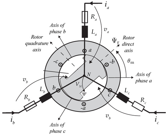
Figure 3.
Synchronous motor circuit scheme and star point voltage.
It is possible to expand the latter three equations and sum them together to obtain the voltage (see Appendix A). This leads to:
Finally, consider that and the assumption that the time interval between the evaluation of two consecutive signals is small enough such that there is not a big change in the derivatives of the stator self-inductances, and phase currents during the interval implies that the last three terms in (6) can be neglected, leading to [30]:
The last assumption is true if, for example, the time interval between two consecutive evaluations is made ten times smaller than the modulation period. Moreover, the voltage clearly embodies the rotor position because the stator self-inductances in the synchronous motor vary as a function of the rotor electrical angle as follows [40]:
where P stands for the number of pole pairs in the machine, stands for the inductance due to the constant component in the air–gap permeance, is due to the phase leakage inductance, and is due to a component in the air–gap permeance, which varies cosinusoidally at twice the rotor electrical angle.
2.2. Standard Voltage Vectors and Voltage between the Star Points
In order to use the DFC method with SVM, it is necessary to study the behavior of the voltage for each of the standard vectors () that can be applied to the synchronous motor. Putting it simply, it is necessary to analyze the behavior of the voltage when each of the voltage space vectors is supplied by the inverter to the synchronous motor terminals. Accordingly, if we consider the two-level inverter depicted in Figure 1, only valid logical states distributed in six sectors () for the three phase windings are possible. The eight logical states lead to eight standard voltage vectors. In particular, there are two voltage vectors where all the windings are connected to the same DC-Link rail (i.e., zero vectors) and the other six vectors that are known as the active vectors [38,40]. Only for illustration purposes is the spatial disposition of the standard vectors used this work in the reference frame shown in Figure 4. Furthermore, resorting to (7) and with reference to Figure 4, the voltage for each of the standard voltage vectors is calculated, and the results can be seen in Table 1. Moreover, the DFC flux linkage signals are calculated from the voltage measured at two different inverter states—more precisely, at two different states that correspond to two different standard voltage vectors. These two standard vectors are applied one after the other with a very small time in between (e.g., tenth of a modulation period) such that the current rate of change between the voltage vectors transition can be neglected. In other words, if the standard vectors are applied one after the other, the phase current can be considered constant for the transition.
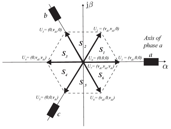
Figure 4.
Standard vectors’ spatial disposition in the reference frame.

Table 1.
Voltage between the star points at different standard space vectors.
For example, the flux linkage signal u can be calculated subtracting the voltage measured when the vector is applied to the machine from the measured when the standard vector was applied. That is:
Under the assumption that the transition interval between the standard vectors is very small, it follows that , , and . Thus, Equation (11) becomes:
From (12), it can be seen that the flux linkage u only depends on the DC-Link voltage and the stator self-inductances that vary with the rotor electrical angle as stated in (8)–(10). Furthermore, in (12), the term is regarded as the offset of the extracted flux linkage u. Due to the fact that the DC-Link voltage is not exactly constant, especially when the DC-Link is supplied through a passive diode–rectifier [41], the offset can vary over the time. For this reason, it is advisable to extract all the signals with the same offset in the measurement sequence. This is with the idea in mind to minimize the DC-Link variation impact over the DFC flux linkage signals [30]. However, there are many possibilities to combine the standard vectors to extract the DFC flux linkage signals (i.e., u,v,w), only a few combinations will extract the three DFC flux linkage signals with the same offset. In effect, the easiest way to extract the DFC flux linkage signals with the same offset is using always a zero vector together with , and as consecutive applied vectors: Specifically:
2.3. Space Vector Modulation with DFC Measurement Sequence
Given that with SVM any space vector can be created by averaging voltage vectors over time in one modulation period, the order of which each voltage vector could appear is not unique. Certainly, the latter is translated into degrees of freedom in the modulation [39]. One particular sequence, the so-called alternated direct inverse SVM sequence [41], is very convenient because it reduces the number of transistors’ commutations within a modulation period and thus reduces the switching losses [42]. The key point in this sequence is that it starts the modulation period with the zero vector and ends the same modulation period with the same zero vector (i.e., the sequence is center aligned). In addition, this sequence brings the big advantage that the time-average value of the phase currents can be measured at the middle of the modulation period without any additional low-pass filters [43]. Obviously, the time-average value of the phase currents is needed for the inner current controllers within a field oriented control scheme. Furthermore, in order to combine the DFC measurement sequence stated by (13)–(15) with the alternated direct inverse SVM pulse pattern, the following algorithm is proposed. First, the reference space vector to be synthesized is given in - coordinates as input to the algorithm. Second, the alternate direct inverse SVM pulse pattern is constructed in the conventional way calculating the turn-on and turn-off times of each phase taking as a base the reference voltage space vector. In this work, the latter was carried out according to the SVM implementation guidelines provided by Quang and Dittrich in [42]. Third, based on the turn-on and turn-off times calculated previously, the total time that each phase’s winding is connected to a positive rail of the DC-Link, namely the phase pulse duration, is computed. Fourth, the DFC measurement sequence is constructed according to (13)–(15) producing three pulse patterns, each with a period equal to one modulation period. On each of these three pulse patterns, the phase pulse duration is held constant as was determined for the first pulse pattern. The idea behind this is to maintain the voltage-time area for each phase winding constant in every modulation period. However, in each of these three pulse patterns, the phase voltages are shifted in such a way to comply with (13)–(15) with the aim to extract the DFC flux linkage signals with the same offset. In order to clarify the pulse patterns’ generation algorithm, let us present a simple example. Consider that a reference voltage space vector that lays on sector 1 (i.e., in Figure 4) is given by its and components. It follows that the right-vector time (), left-vector time (), and zero-vector time () can be calculated as follows [42]:
Based on these results, the alternated direct inverse SVM pulse pattern can be constructed calculating the turn-on and turn-off times for each phase as:
Then, the phase pulse duration needed to construct the DFC pulse patterns can be obtained:
After all these calculations, the four pulses are generated as is shown in Figure 5. Clearly, the first of the pulse patterns is the alternated direct inverse SVM pulse pattern that is used to sample the phase currents.
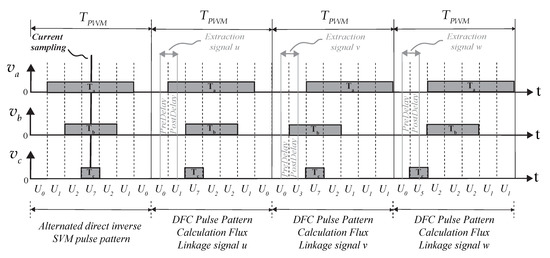
Figure 5.
Inverter states for flux linkage measurement within the enhanced measurement sequence (SVM combinated with DFC).
Next, the first DFC pulse to extract the flux linkage signal u is generated according to (13) maintaining the pulse durations calculated by (25) through (27). Similarly, the next two DFC pulses are generated based on (14) and (15) to extract the DFC flux linkage signals v and w, respectively. Of course, the pulse duration for each phase is kept constant in the last two pulses as well. Notice that conventional SVM uses only the standard vectors , , and to synthesize a voltage vector in sector 1. However, the SVM-based DFC measurement sequence unfortunately introduces the standard vectors and in the last two modulation periods. Granted that the use of standard vectors that are not part of the sector will cause the resultant space vector to deviate from the reference. However, this deviation will be small, and it is accepted for the sake of keeping the pulse pattern generation algorithm as simple as possible.
3. Sensorless Speed Closed Loop Control with Field Oriented Control and SVM-Based DFC Measurement Sequence
It is widely known that the most effective way to perform speed control over a synchronous motor is resorting to the rotating reference frame or dq frame [5,39,40]. This implies that the exact electrical rotor position is needed to transform all the variables to dq coordinates using the Clarke–Park transformation [41]. On this basis, Equations (28)–(31) show the relations between the synchronous motor’s variables in the dq coordinates [40]:
where is the phase winding resistance, and are the direct and quadrature inductances, and and are the direct and quadrature currents. Furthermore, is the electrical angular speed, is the rotor flux established by the permanent magnets in the rotor, and is the mechanical angular speed. Finally, is the electromagnetic torque produced by the synchronous motor, and is the load torque. Of course, from (30), it can be inferred that the electromagnetic torque can be changed rapidly by manipulating if is zero. From (31), the angular acceleration can be changed by manipulating appropriately the electromagnetic torque . All in all, the synchronous motor’s speed control reduces to the control of the and currents. Certainly, the electrical rotor position needed to carry out the control in the rotating reference frame can be supplied by DFC.
3.1. Rotor Position Estimation Using DFC
3.2. DFC-Based Rotor Speed Estimation
The rotor speed needed by the speed control loop can be calculated from two consecutive electrical rotor positions outputted by DFC. However, in order to improve the speed calculation accuracy, we have employed an average moving filter (MAF) with 16 samples to smooth the DFC estimated position. From the smoothed position signals, the rotor speed can be computed as:
3.3. Sensorless Speed Closed Loop Control with Field Oriented Control Structure
Speed control of synchronous motors with field oriented control is inherently a cascaded control loop, where the outer speed controller sets the reference to the inner current control loop on the q-axis. In fact, this control structure is illustrated in Figure 6. Obviously, the particularity of Figure 6 is that the position sensorless speed control is realized using the SVM-based DFC measurement sequence. Notice that the time-average phase currents can be obtained only within a time frame of four switching periods. This represents a disadvantage in comparison with conventional field oriented control based in standard SVM, which obtains the time-average phase currents at every switching period. Thus, the current controllers for sensorless field oriented control based on DFC need to be designed with a bandwidth four times smaller than for conventional field oriented control. Furthermore, in the control structure, the speed is calculated according to (33). Nonetheless, the calculated speed is filtered once again by a low pass filter (LPF) in the closed loop to improve the speed reference tracking. With this in mind, the speed controller, current controllers, and axis decoupling feed-forward controllers in this work are designed according to [39]. Moreover, in case of voltage saturation in the demanded voltages by the current controllers, the voltages and are truncated limiting the modulation ratio splitting the limitation between both voltages components as follows [42]:
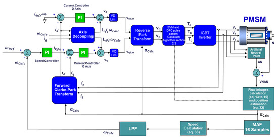
Figure 6.
Sensorless speed control with SVM-based DFC measurement sequence.
4. Finite Element Model of the Synchronous Machine
The proposed SVM-based DFC measurement sequence that extracts the DFC flux linkages’ signals with the same offset level is validated through computer simulation in this paper. As DFC exploits the fact that the stator’s self-inductances vary as a function of the rotor position, it is necessary to have a machine model that reproduces with high fidelity the electromagnetic phenomena that occur in the real machine. The latter is actually possible using a finite element model of the synchronous machine. In particular, we have modeled a real Wound Rotor Separated Excited Synchronous machine (WRSESM) using the finite element (FE) method in ANSYS Maxwell. Certainly, in the future, we will use the developed WRSESM model to study the behavior of DFC varying the rotor flux changing the field current. However, in this work, for all the field oriented control simulations that we have performed, we have kept the WRSESM’s field current constant at 0.4 A. Therefore, in reality, the WRSESM behaved effectively as a PMSM for all the field oriented control studies presented in this paper. Furthermore, the company WUEKRO GmbH supplied us with a real WRSESM (see Figure 7) whose nominal parameters can be seen in Table 2.
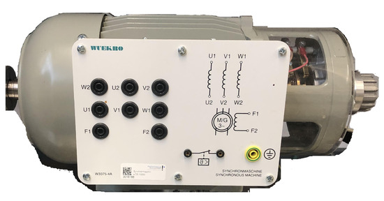
Figure 7.
WUEKRO Wound Rotor Separated Excited Synchronous Motor (WRSESM).
Table 2.
WUEKRO WRSESM—Nominal parameters.
Furthermore, and in addition to the real WRSESM, the constructional details of the machine were also provided. Specifically, the stator and rotor geometries, the magnetic materials used (M800-50A non-oriented electrical steel for the stator and steel ST37 for the rotor), and windings’ schemes were disclosed by the manufacturer. With all this information (which can be found in Appendix B), we have developed the FE model of the WRSESM. In fact, the developed FE model can be seen in Figure 8.
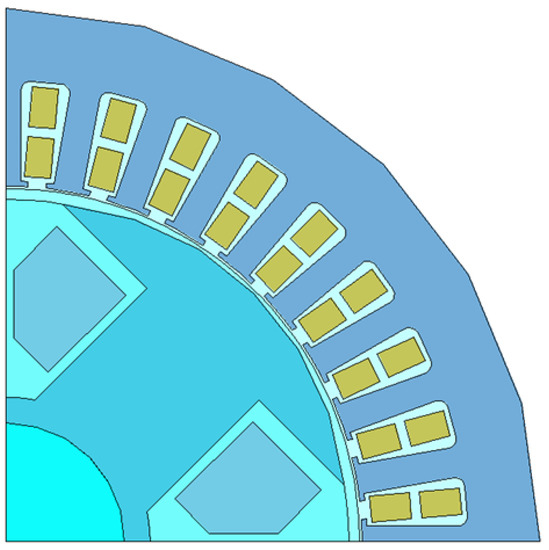
Figure 8.
Quarter finite element model of the WRSESM developed in ANSYS Maxwell.
4.1. WRSESM Model Reduction
It is granted that the WRSESM has four poles. However, in ANSYS Maxwell, we have created only one quarter of the WRSESM four pole’s symmetric structure. Actually, in the real machine, the magnetic poles in the stator and rotor alternate between north and south poles during the entire operation. Indeed, the same behavior can be reproduced in ANSYS Maxwell configuring negative master/slave boundary conditions in the one quarter FE model. This allows for reducing the model’s calculation complexity and the processing time without comprising the high simulation’s fidelity brought by the finite element method [44].
4.2. Model Validation
Furthermore, the FE model was validated against the real WRSESM through two different tests, namely the open-circuit test and the short-circuit test. The open-circuit and short-circuit tests were performed according to [40] driving the FE model and the real machine at 1500 RPM and varying the field current from 0 A to its nominal value of 0.6 A. Actually, Figure 9 and Figure 10 show the validation results for the open-circuit test and short-circuit test, respectively. From both figures, it is possible to see that the open-circuit voltages and the short-circuit currents of the FE model closely follow the values measured in the real WRSESM. In particular, the tests’ comparison shows a maximum relative error in the open-circuit test of 7%, and a maximum relative error in the open-circuit test of 5%. However, notice that the mentioned relative errors are valid for field winding currents larger than 0.2 A.
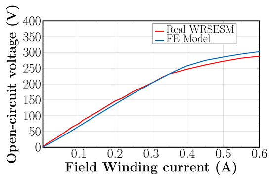
Figure 9.
Open-circuit characteristics of the FE model and real WRSESM.
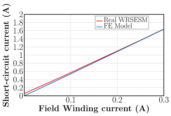
Figure 10.
Short-circuit characteristics of the FE model and real WRSESM.
5. Simulation Validation
The DFC-based sensorless speed control with field oriented control is validated through a co-simulation between ANSYS Maxwell and ANSYS Simplorer (see Figure 11)—specifically, through a transient coupling simulation between the FE model of the motor created in Maxwell and a power electronics circuit implemented in Simplorer. Actually, the FE model is interfaced through passive resistors to the two-level inverter. These resistors have to have the same value as the winding resistance in the real WRSESM. The latter is necessary because the co-simulation does not support direct connection of voltage or current sources to the FE model pins [44]. In addition, three resistors of 470 k are used to construct the artificial star point, and the other three resistors of 470 k are used to measure the voltages that are fed to the machine to build the voltage difference . Moreover, the control logic (see Figure 6) is implemented in C++ language in a Simplorer C-model block. This block includes the code for the speed controller, current controllers, and the SVM-based DFC pulse pattern generator. In addition, the speed calculation based on the DFC estimated position alongside the moving average filter and LPF filter needed to smooth the speed signal are also implemented in the C-model block. In any case, the co-simulation between ANSYS Simplorer and Maxwell is carried out by a data exchange between the Simplorer and Maxwell solvers in the simulation time step. On the one hand, ANSYS Simplorer sees in each simulation time step the FE motor windings in each phase as a Thevenin equivalent circuit with a specific voltage-source, a resistance and an inductance.
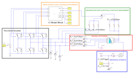
Figure 11.
Sensorless speed control with field oriented control and SVM-based DFC measurement sequence, Simplorer-Maxwell co-simulation model.
On the other hand, ANSYS Maxwell sees each phase of the Simplorer circuit as a Norton equivalent circuit with a specified source-current and an admittance. In the mechanical physical domain, the mechanical torque is set by Maxwell to Simplorer. Moreover, the co-simulation approach updates automatically the values for the windings self and mutual inductances after each time step depending on the rotor position. The inductances’ value automatic update is carried out by ANSYS Maxwell as follows: after each time step, the permeabilities in each of the FE model’s elements are frozen. Then, a current of 1 A is applied in each winding, one at a time, while currents on the other windings are zero. For the applied current, each winding flux linkage is calculated for the model’s given position, and, afterwards, the values for the self and mutual inductances are recalculated for the equivalent circuit seen by Simplorer. Furthermore, Table 3 shows the parameters for the power electronic circuit, SVM-based DFC pulse pattern generation, speed controller, and current controllers used for the simulation validation.
Table 3.
Sensorless speed control with DFC—Simulation parameters.
5.1. Comparison: SVM-Based DFC and SPWM-Based DFC
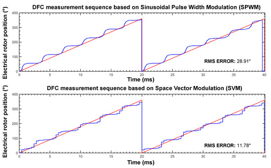
In order to compare the performance of the proposed SVM-based DFC sequence described in Section 2.3 with the original DFC measurement sequence proposed in [27], the model in Figure 11 was simulated using the parameters described in Table 3. For this comparison, we set a speed reference of 1500 RPM for the synchronous machine. On this basis, the rotor position estimated by both methods when the machine reaches its steady state speed of 1500 RPM can be seen in Figure 12. It turns out that the Root Mean Square (RMS) of the position estimation error values is taken as a statistical measure to compare both DFC measurement sequences. Furthermore, Figure 12 shows that, at a speed of 1500 RPM, the modified DFC-based space modulation sequence reaches an RMS error in the rotor position estimation of 11.78°, whereas the original measurement DFC based on SPWM exhibits an RMS error of 28.91° on the rotor position estimation. The DFC measurement sequence based on SVM, which extracts all the DFC flux linkage signals with the same offset and the one proposed in this article, outperforms the original DFC measurement sequence based on SPWM, which extracts the DFC flux linkage signals with a different offset. The latter has already been discussed in Section 2.2 and can be verified resorting to Equations (13)–(15) for the SVM-based DFC measurement sequence, and Equations (16)–(18) for the SPWM-based DFC measurement sequence.
5.2. Sensorless Field Oriented Control with SVM-Based DFC for High Speed Reference
Two additional simulations are carried out using the model depicted in Figure 11 using the DFC method to estimate the rotor position and to calculate the rotor’s speed. Of course, one of the advantages of the high-fidelity FE model connected to Simplorer is that we can evaluate the real position and the real speed of the synchronous machine during the simulation. This information can be compared with the DFC generated signals in order to evaluate the performance of the sensorless control field oriented control with DFC. Furthermore, in the second simulation, we have set the speed reference equal to 1200 RPM at t = 0 ms and a load torque step from = 0 Nm to = 0.1 Nm at t = 50 ms. In this regard, Figure 13 shows the simulation results of the speed control where the real speed of the machine is depicted together with the speed reference. For the same simulation, Figure 14 shows the speed calculated based on the proposed DFC method against the real speed of the machine. From Figure 13, it can be seen that the real speed of the machine matches the reference of 1200 RPM approximately at t = 130 ms. On the other hand, Figure 14 shows that the speed calculated based on the DFC estimated rotor position signal follows the real speed of the machine reasonably well. From the figure, it can be seen that the speed calculated according to the proposed DFC method deviates 10% from the real speed of the machine. Moreover, the DFC flux linkage signals calculated according to (13)–(15) during this second simulation can be seen in Figure 15.
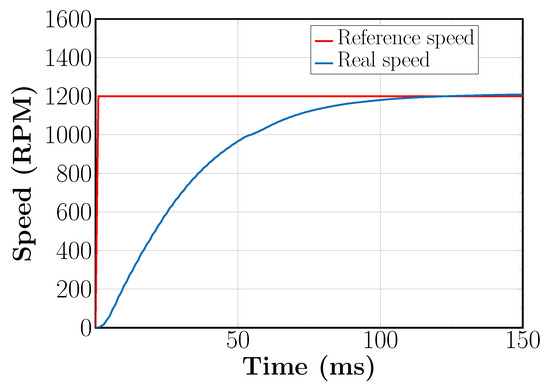
Figure 13.
Sensorless speed control for 1200 RPM, speed reference and real speed of the machine.
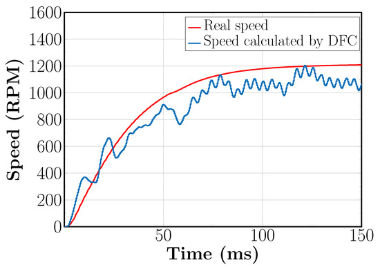
Figure 14.
Sensorless speed control for 1200 RPM, real speed of the machine and speed calculated by DFC.
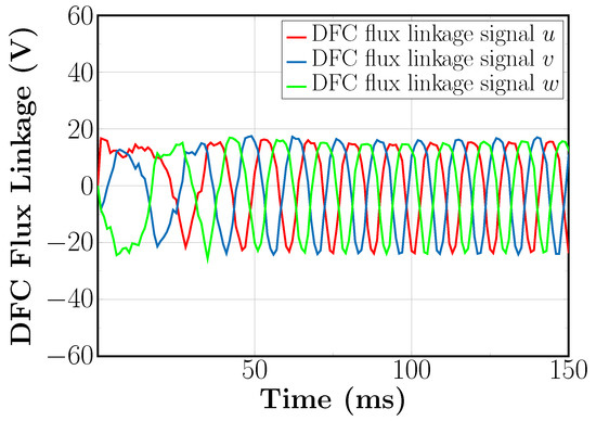
Figure 15.
Sensorless speed control for 1200 RPM, DFC flux linkage signals.
During the acceleration phase, between t = 0 ms and t = 50 ms, it can be seen that the DFC flux linkage signals have a very low frequency due to the fact that the rotor is accelerating from standstill. Furthermore, it can inferred that the three DFC flux linkage signals always add to zero at any instant of time. Based on those DFC flux linkage signals, the estimated rotor position has been computed according to (32), and it can be seen in Figure 16. In addition, in the figure, the real electrical angle of the rotor is depicted for evaluation purposes. From the figure, it can be seen that the estimated electrical position closely follows the real rotor electrical position, especially after t = 75 ms. Clearly, there are certain ripples or oscillations on the estimated rotor position that are inherent to the frequencies involved in the DFC flux linkage signals, with a prominent second and fourth harmonic components of the speed of the machine. The latter was explained in detail by Mantala in [30]. Next, Figure 17 shows the three-phase currents supplied by the inverter to the synchronous motor in the stationary frame. In fact, the frequency of the supplied currents increases as the machine’s rotor accelerates from standstill as is expected. It should be noticed that the shape of the supplied currents follows a sinusoidal shape, although the estimated rotor position deviates a little from the real rotor position. Moreover, the synchronous motor’s currents transformed to the rotating reference frame can be seen for the direct (d-axis) and for the quadrature axis (q-axis) in Figure 18 and Figure 19 respectively.
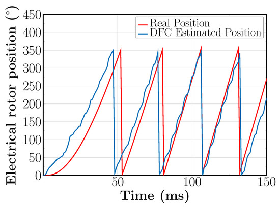
Figure 16.
Sensorless speed control for 1200 RPM, real electrical rotor position and DFC estimated rotor position.
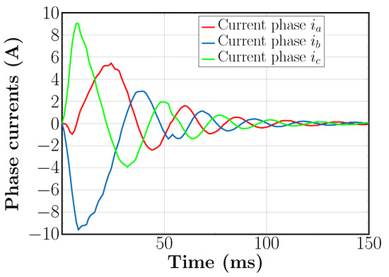
Figure 17.
Sensorless speed control for 1200 RPM, stator three-phase currents.
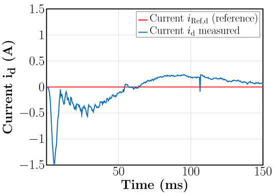
Figure 18.
Sensorless speed control for 1200 RPM, current on the d-axis.
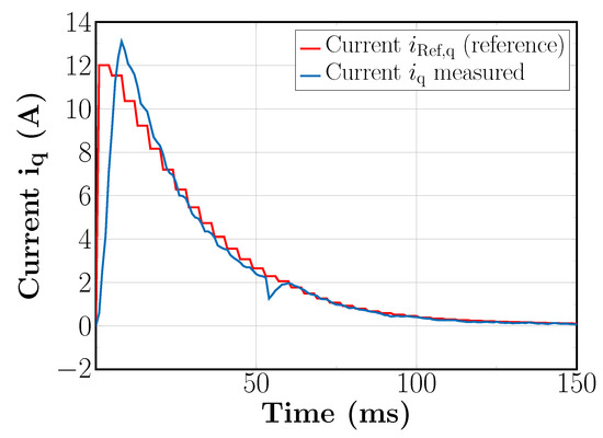
Figure 19.
Sensorless speed control for 1200 RPM, current on the q-axis.
Obviously, we can see in Figure 18 that the measured current deviates a little from its zero reference at the beginning of the simulation. The latter is due to the fact that, at the beginning of the simulation, the deviation between the rotor estimated position and the real rotor position is large. After t = 50 ms, the DFC outputted rotor position better approaches the real rotor position, and thus the d-axis currents remain closer to its zero reference as expected due to the action of the d-axis current controller. Finally, it is possible to see in Figure 19 that is proportional to the torque produced by the synchronous motor, which is depicted in Figure 20. Notice that, at t = 50 ms, there is a small deviation on the q-axis current and in the motor’s torque due to the effect of the load torque at the shaft of the synchronous machine. Altogether, it can be seen that the proposed sequence is effective to perform sensorless speed control with field oriented control at high speeds—for this last simulation, at a speed of 80% of the nominal speed of the synchronous machine.
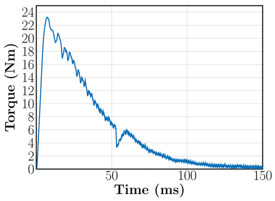
Figure 20.
Sensorless speed control for 1200 RPM, torque produced by the synchronous motor.
5.3. Sensorless Field Oriented Control with SVM-Based DFC for Low Speed Reference
The third simulation performed in this paper is carried out at a low speed. Specifically, we have set the reference for the second simulation as 100 RPM from t = 0 s to t = 200 ms. Moreover, for the simulation at low speed, the load torque was kept constant at = 0.1 Nm during the entire simulation time span. In effect, Figure 21 shows the reference speed for this third simulation and the real speed of the machine obtained from the FE model. In simple terms, Figure 21 is analogous to Figure 13 but for a reference speed of 100 RPM. On the same note, Figure 22 shows the real speed and the speed calculated based on DFC signals for the same simulation. Once again, Figure 22 is analogous to Figure 14 in the previous simulation. Although the speed calculated by DFC deviates in Figure 22 a little bit from the real speed of the machine, the average value of the DFC calculated speed matches the real speed of the machine. Putting it simply, on average, the sensorless speed control loop follows the reference of 100 RPM. The latter can be improved, adjusting the cutoff frequency of the low pass filter within the speed control loop.
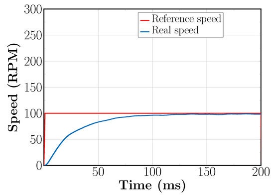
Figure 21.
Sensorless speed control for 100 RPM, speed reference and real speed of the machine.
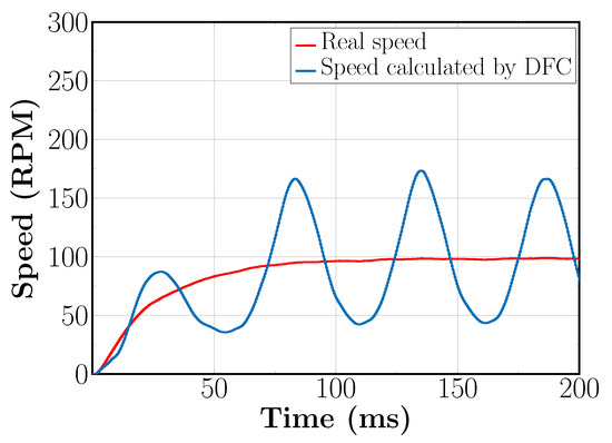
Figure 22.
Sensorless speed control for 100 RPM, real speed of the machine and speed calculated by DFC.
Furthermore, for the third simulation, Figure 23 shows the extracted DFC flux linkage signals for the experiment with a speed reference of 100 RPM. It can be seen that the amplitude of the DFC flux linkage signals reaches 20 V. In addition, as in the previous simulation, the DFC flux linkage signals sum to zero at any moment in time. From these DFC flux linkage signals, the rotor position can be estimated for the low speed simulation. In fact, the estimated rotor position for this third simulation can be seen in Figure 24. In the same figure, once again, the real position is also plotted to evaluate the performance of the DFC outputted rotor position. From the figure, it can be inferred that the DFC estimated rotor position follows the real rotor electrical position reasonably well.
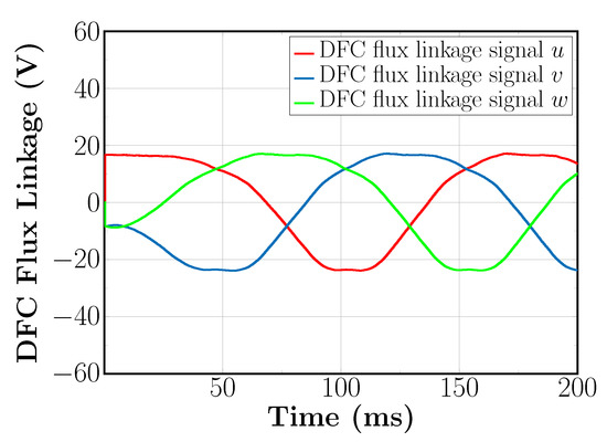
Figure 23.
Sensorless speed control for 100 RPM, DFC flux linkage signals.
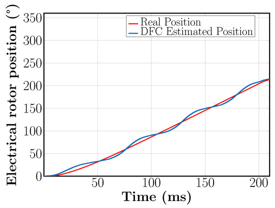
Figure 24.
Sensorless speed control for 100 RPM, real electrical rotor position and DFC estimated rotor position.
Finally, for this low speed simulation, Figure 25 is analogous to Figure 17 and shows the three-phase currents supplied to the synchronous motor in the stationary frame. Clearly, after the transients to accelerate the rotor, the currents falls to almost a value of zero due to the fact that the load torque is small (only 0.1 Nm). Conversely, Figure 26 and Figure 27 show the currents supplied to the synchronous motor in the rotating reference frame using the rotor position obtained through the DFC method to perform the transformation. Similar to the second simulation, Figure 26 shows the behavior of the current on the d-axis which is regulated to zero amperes. In this case, the are no large deviations from the zero reference because, at low speeds, the DFC outputted rotor position is always very close to the real rotor position. On the other hand, Figure 27 shows the current on the q-axis supplied to the motor. Obviously, this current is directly proportional to the electromagnetic torque that is generated by the synchronous motor. The latter can be verified by inspecting Figure 28 which shows the torque produced by the synchronous motor for this third simulation. Additionally, in Figure 28, we can see the positive torque to accelerate the rotor from standstill to 100 RPM, approximately from t = 0 s to t = 50 ms. On the whole, the simulation results presented in Figure 21, Figure 22, Figure 23, Figure 24, Figure 25, Figure 26, Figure 27 and Figure 28 show that the proposed SVM-based DFC measurement sequence is also effective to drive the synchronous motor at low speeds—specifically for this simulation at a speed of 6.6% of the synchronous motor’s nominal speed.
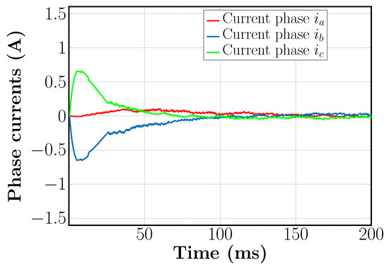
Figure 25.
Sensorless speed control for 100 RPM, stator currents in stationary frame.
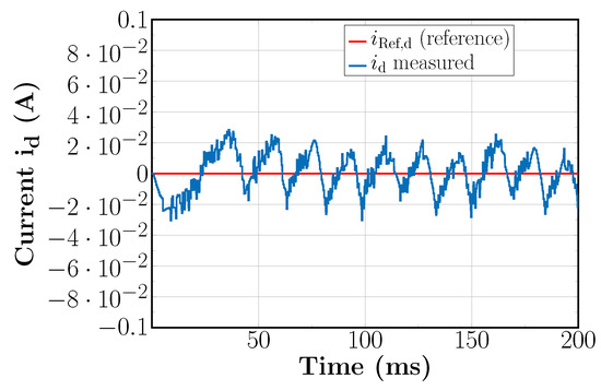
Figure 26.
Sensorless speed control for 100 RPM, current on the d-axis.
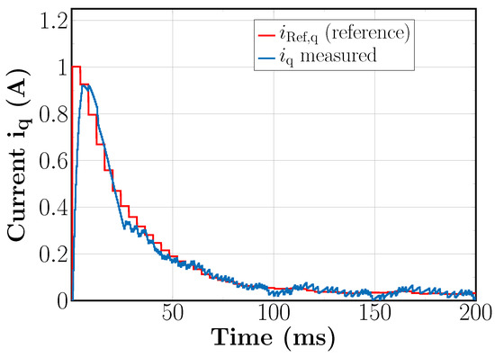
Figure 27.
Sensorless speed control for 100 RPM, current on the q-axis.
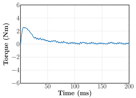
Figure 28.
Sensorless speed control for 100 RPM, synchronous motor’s generated torque.
6. Conclusions
This paper has walked through sensorless speed control with field oriented control for synchronous motors using a SVM-based Direct Flux Control measurement sequence. In particular, in this paper we have used the Direct Flux Control method to obtain the rotor electrical position needed to perform field oriented control. In addition, the rotor position obtained by DFC is also utilized to calculate the actual rotor speed and close the sensorless speed control loop. In contrast with previous work, in this paper we have combined the Direct flux method with space vector modulation within the field oriented control scheme. To this end, we have performed an analysis of the voltage for each of the eight standard voltage vectors that can be applied to a synchronous motor using a two-level inverter. Recall that the voltage is the key signal to calculate the DFC flux linkage signals. It is from those DFC flux linkage signals that the rotor position can be finally estimated. Moreover, after the analysis of the response to each of the standard vectors, we have proposed a SVM-based DFC measurement sequence. Actually, the SVM-based DFC measurement sequence consists of four modulation switching periods. In the first period, a conventional alternated direct inverse SVM pulse pattern is generated. From this first pulse pattern, the time-average phase currents (i.e., phase currents without ripple) can be measured and used as feedback signals in the inner current controllers. Next, three pulse patterns with a duration of one switching period each are generated holding the phase pulse duration constant as in the first switching period. However, the phase pulses are shifted in these last three switching periods in such a way that the three DFC flux linkage signals can be extracted with an offset of . Extracting all the DFC flux linkage signals with the same offset is very advantageous because the rotor position estimation accuracy is improved. Furthermore, this paper has shown the sensorless speed control structure for a synchronous motor that uses the SVM-based DFC measurement sequence. This sensorless speed control structure has been validated through computer simulation. The simulation is made possible by a coupling simulation between an FE model of the motor created in ANSYS Maxwell and a power electronics circuit created in ANSYS Simplorer. Furthermore, using the Simplorer-Maxwell co-simulation, the sensorless speed control structure based on SVM and DFC has been tested for two cases. First, a test was carried out with a reference speed of 1200 RPM (i.e., 80% of the machine nominal speed) which can be considered as a high speed setpoint for a four-pole machine. In the second case, we have set a reference speed equal to 100 RPM (i.e., 6.6% of the machine nominal speed), namely a low speed reference, to the machine. Altogether, the simulation results have shown that, in both cases, the proposed DFC algorithm was able to estimate the rotor electrical position reasonably well. Additionally, the proposed sensorless speed control scheme proposed was also able to command the synchronous motor rotor’s speed close to the speed reference at high and low speeds. Finally, and due to the large amount of time needed to perform simulations with the FE’s model, future work will address the performance of the proposed control scheme at other operating points (e.g., different load conditions and other reference speeds).
Author Contributions
Conceptualization, R.G.I.; methodology, R.G.I.; software, R.G.I.; validation, R.G.I.; formal analysis, R.G.I.; investigation, R.G.I.; resources, P.T.; data curation, R.G.I.; writing—original draft preparation, R.G.I.; writing—review and editing, R.G.I.; visualization, R.G.I.; supervision, P.T.; project administration, P.T. All authors have read and agreed to the published version of the manuscript.
Funding
This research received no external funding.
Data Availability Statement
Data available on request due to privacy restrictions.
Acknowledgments
The authors express their gratitude to Marvin Cruse for his suggestions during the development of this work.
Conflicts of Interest
The authors declare no conflict of interest.
Abbreviations
The following abbreviations are used in this manuscript:
| DFC | Direct Flux Control |
| SVM | Space Vector Modulation |
| SM | Synchronous Machines |
| PMSM | Permanent Magnet Synchronous Machines |
| PWM | Pulse Width Modulation |
| SPWM | Sinusoidal Pulse Width Modulation |
| EMI | Electromagnetic Interference |
| FEM | Finite Element Model |
| FE | Finite Element |
Appendix A. Machine’s Star Voltage Equation
This appendix shows the detailed derivation of the equation for the machine star voltage based on the phase voltage equations of the machine in the reference frame. It turns out that (3) to (5) can be further expanded as:
Under the condition that the sum of the phase current derivatives is zero, in other words:
From the last equation, the voltage at the star point of the machine can be obtained as:
Appendix B. Finite Element Model (FEM) Synchronous Machine Data
STATOR DATA
Number of Stator Slots: 36
Outer Diameter of Stator (mm): 135
Inner Diameter of Stator (mm): 90
Type of Stator Slot: 4
Dimension of Stator Slot
hs0 (mm): 0.62
hs1 (mm): 0
hs2 (mm): 11.5
bs0 (mm): 2.3
bs1 (mm): 4.16538
bs2 (mm): 6.17762
rs (mm): 1.2
Top Tooth Width (mm): 3.79681
Bottom Tooth Width (mm): 3.7917
Number of Sectors per Lamination: 1
Skew Width (slots): 0
Length of Stator Core (mm): 200
Stacking Factor of Stator Core: 0.96
Type of Steel: M800 50A
Press board thickness (mm): 0
Magnetic press board No
Number of Air Ducts: 0
Width of Air Ducts (mm): 0
STATOR-WINDING DATA
End Length Adjustment (mm): 5
End-Coil Clearance (mm): 3
Number of Parallel Branches: 1
Type of Coils: 20
Coil Pitch: 1
Number of Conductors per Slot: 70
Number of Wires per Conductor: 1
Wire Diameter (mm): 0.633
Wire Wrap Thickness (mm): 0
Wedge Thickness (mm): 1
Slot Liner Thickness (mm): 0.4
Layer Insulation (mm): 0.5
Net Slot Area (mm): 44.2774
Slot Fill Factor (%): 63.3466
Limited Slot Fill Factor (%): 75
Stator Winding Factor: 0.901912
ROTOR DATA
Minimum Air Gap (mm): 0.7
Inner Diameter (mm): 30
Length of Rotor (mm): 111
Stacking Factor of Iron Core: 1
Type of Steel: steel ST37
Polar Arc Offset (mm): 5
Ratio of Max. to Min. Air Gap: 2.46436
Mechanical Pole Embrace: 0.784201
Pole-Shoe Width (mm): 50
Pole-Shoe Height (mm): 9.1
Pole-Body Width (mm): 20
Pole-Body Height (mm): 20
Second Air Gap (mm): 0
Magnetic Shaft: Yes
FIELD-WINDING DATA
Number of Parallel Branches: 1
Winding Type: Round-Wire Coil
Wire Diameter (mm): 0.355
Number of Wires: 1
Number of Turns per Pole: 1250
Wire Wrap Thickness (mm): 0
Under-Pole-Shoe Insulation (mm): 0.5
Pole-Body-Side Insulation (mm): 0.3
Winding Control Width (mm): 14.5464
Winding Control Height (mm): 19
Clearance between Windings (mm): 0.5
Inside Corner Radius (mm): 6
End Core-Coil Clearance (mm): 0
MATERIAL CONSUMPTION
Armature Copper Density (kg/m): 8900
Field Copper Density (kg/m): 8900
Damper Bar Material Density (kg/m): 2700
Damper Ring Material Density (kg/m): 2700
Armature Core Steel Density (kg/m): 7800
Rotor Core Steel Density (kg/m): 7872
Armature Copper Weight (kg): 1.5855
Field Copper Weight (kg): 1.39334
Damper Bar Material Weight (kg): 0
Damper Ring Material Weight (kg): 0
Armature Core Steel Weight (kg): 8.25956
Rotor Core Steel Weight (kg): 1.85934
Total Net Weight (kg): 13.0977
Armature Core Steel Consumption (kg): 28.5203
Rotor Core Steel Consumption (kg): 7.3316
WINDING ARRANGEMENT
Average coil pitch is: 7
Angle per slot (elec. degrees): 20
Phase-A axis (elec. degrees): 90
First slot center (elec. degrees): 0
Maximum number of layers: 39
Maximum number of turns per layer: 50
TRANSIENT FEA INPUT DATA
For Armature Winding:
Number of Turns: 420
Parallel Branches: 1
Terminal Resistance (ohm): 14.6902
End Leakage Inductance (H): 0.000617567
For Pole Winding:
Number of Turns: 5000
Parallel Branches: 1
Terminal Resistance (ohm): 391.507
End Leakage Inductance (H): 0.429572
2D Equivalent Value:
Equivalent Model Depth (mm): 111
Equivalent Stator Stacking Factor: 1.72973
Equivalent Rotor Stacking Factor: 1
References
- Liu, Y.; Laghrouche, S.; Depernet, D.; Djerdir, A.; Cirrincione, M. Disturbance-Observer-Based Complementary Sliding-Mode Speed Control for PMSM Drives: A Super-Twisting Sliding-Mode Observer-Based Approach. IEEE J. Emerg. Sel. Top. Power Electron. 2021, 9, 5416–5428. [Google Scholar] [CrossRef]
- Wang, G.; Zhang, G.; Xu, D. Position Sensorless Control Techniques for Permanent Magnet Synchronous Machine Drives; Springer: Singapore, 2020; pp. 2–10. [Google Scholar]
- Tapani, J.; Hrabovcova, V.; Pyrhonen, J. Design of Rotating Electrical Machines; John Wiley & Sons: Hoboken, NJ, USA, 2013. [Google Scholar]
- Li, C.; Elbuluk, M. A sliding mode observer for sensorless control of permanent magnet synchronous motors. In Proceedings of the Conference Record of the 2001 IEEE Industry Applications Conference—36th IAS Annual Meeting (Cat. No. 01CH37248), Chicago, IL, USA, 30 September–4 October 2001; Volume 2, pp. 1273–1278. [Google Scholar]
- Weidauer, J.; Messer, R. Electrical Drives: Principles, Planning, Applications, Solutions; John Wiley & Sons: Hoboken, NJ, USA, 2014; pp. 152–153. [Google Scholar]
- Sandre-Hernandez, O.; Morales-Caporal, R.; Rangel-Magdaleno, J.; Peregrina-Barreto, H.; Hernandez-Perez, J.N. Parameter identification of PMSMs using experimental measurements and a PSO algorithm. IEEE Trans. Instrum. Meas. 2015, 64, 2146–2154. [Google Scholar] [CrossRef]
- Lara, J.; Xu, J.; Chandra, A. Effects of rotor position error in the performance of field-oriented-controlled PMSM drives for electric vehicle traction applications. IEEE Trans. Ind. Electron. 2016, 63, 4738–4751. [Google Scholar] [CrossRef]
- Podder, A.; Pandit, D. Study of Sensorless Field-Oriented Control of SPMSM Using Rotor Flux Observer & Disturbance Observer Based Discrete Sliding Mode Observer. In Proceedings of the 2021 IEEE 22nd Workshop on Control and Modelling of Power Electronics (COMPEL), Cartagena, Colombia, 2–5 November 2021; pp. 1–8. [Google Scholar]
- DPulle, W.; Darnell, P.; Veltman, A. Applied Control of Electrical Drives; Springer: Berlin/Heidelberg, Germany, 2015; pp. 18–31. [Google Scholar]
- Jung, S.; Nam, K. PMSM Control Based on Edge-Field Hall Sensor Signals Through ANF-PLL Processing. IEEE Trans. Ind. Electron. 2011, 58, 5121–5129. [Google Scholar] [CrossRef]
- Sul, S.-K. Control of Electric Machine Drive System; IEEE Press: Piscataway, NJ, USA, 2011. [Google Scholar]
- Sul, S.-K. Motor Drive and Sensorless Control; 3rd Asian PhD School on Advanced Power Electronics: Chengdu, China, 2021. [Google Scholar]
- Wolf, C.M.; Lorenz, R.D. Using the Motor Drive as a Sensor to Extract Spatially Dependent Information for Motion Control Applications. IEEE Trans. Ind. Appl. 2011, 47, 1344–1351. [Google Scholar] [CrossRef]
- Qu, L.; Qiao, W.; Qu, L. An Enhanced Linear Active Disturbance Rejection Rotor Position Sensorless Control for Permanent Magnet Synchronous Motors. IEEE Trans. Power Electron. 2020, 35, 6175–6184. [Google Scholar] [CrossRef]
- Rashed, M.; MacConnell, P.F.A.; Stronach, A.F.; Acarnley, P. Sensorless Indirect-Rotor-Field-Orientation Speed Control of a Permanent-Magnet Synchronous Motor With Stator-Resistance Estimation. IEEE Trans. Ind. Electron. 2007, 54, 1664–1675. [Google Scholar] [CrossRef]
- Chi, S.; Zhang, Z.; Xu, L. Sliding-Mode Sensorless Control of Direct-Drive PM Synchronous Motors for Washing Machine Applications. IEEE Trans. Ind. Appl. 2009, 45, 582–590. [Google Scholar] [CrossRef]
- Ye, S.; Yao, X. An Enhanced SMO-Based Permanent-Magnet Synchronous Machine Sensorless Drive Scheme With Current Measurement Error Compensation. IEEE J. Emerg. Sel. Top. Power Electron. 2021, 9, 4407–4419. [Google Scholar] [CrossRef]
- Raca, D.; Garcia, P.; Reigosa, D.D.; Briz, F.; Lorenz, R.D. Carrier signal selection for sensorless control of PM synchronous machines at zero and very low speeds. Proc. IEEE Ind. Appl. 2009, 46, 167–178. [Google Scholar] [CrossRef]
- Liu, J.M.; Zhu, Z.Q. Sensorless control strategy by square-waveform high-frequency pulsating signal injection into stationary reference frame. IEEE J. Emerg. Sel. Topics Power Electron. 2014, 2, 171–180. [Google Scholar] [CrossRef]
- Xu, P.L.; Zhu, Z.Q. Novel square-wave signal injection method using zero-sequence voltage for sensorless control of PMSM drives. IEEE Trans. Ind. Electron. 2016, 63, 7444–7454. [Google Scholar] [CrossRef]
- Schrödl, M.; Lambeck, M. Statistic properties of the INFORM-method in highly dynamics sensorless PM motor control applications down to standstill. Eur. Power Electron. Drives 2003, 13, 22–29. [Google Scholar] [CrossRef]
- Zentai, A.; Daboczi, T. Improving INFORM calculation method on permanent magnet synchronous machines. In Proceedings of the 2007 IEEE Instrumentation & Measurement Technology Conference (IMTC 2007), Warsaw, Poland, 1–3 May 2007; pp. 1–6. [Google Scholar]
- Thiemann, P.; Mantala, C.; Mueller, T.; Strothmann, R.; Zhou, E. Direct Flux Control (DFC): A New Sensorless Control Method for PMSM. In Proceedings of the 2011 46th International Universities’ Power Engineering Conference (UPEC), Soest, Germany, 5–8 September 2011; pp. 1–6. [Google Scholar]
- Müller, T.; See, C.; Ghani, A.; Bati, A.; Thiemann, P. Direct flux control–sensorless control method of PMSM for all speeds–basics and constraints. Electron. Lett. 2017, 53, 1110–1111. [Google Scholar] [CrossRef]
- Grasso, E.; Palmieri, M.; Mandriota, R.; Cupertino, F.; Nienhaus, M.; Kleen, S. Analysis and Application of the Direct Flux Control Sensorless Technique to Low-Power PMSMs. Energies 2020, 13, 1453. [Google Scholar] [CrossRef]
- Robeischl, E.; Schroedl, M. Optimized INFORM measurement sequence for sensorless PM synchronous motor drives with respect to minimum current distortion. IEEE Trans. Ind. Appl. 2004, 40, 591–598. [Google Scholar] [CrossRef]
- Strothmann, R. Device for Obtaining Information about the Rotor Position of Electric Machines. DE Patent WO 2007/073854, 5 July 2007. [Google Scholar]
- Thiemann, P.; Mantala, C.; Mueller, T.; Strothmann, R.; Zhou, E. Sensorless control for buried magnet PMSM based on direct flux control and fuzzy logic. In Proceedings of the 8th IEEE Symposium on Diagnostics for Electrical Machines, Power Electronics & Drives, Bologna, Italy, 5–8 September 2011; pp. 405–412. [Google Scholar]
- Müller, T.; See, C.; Ghani, A.; Thiemann, P. Simulation of PMSM in maxwell 3D/simplorer to optimize direct flux control. In Proceedings of the 2017 IEEE 26th International Symposium on Industrial Electronics (ISIE), Edinburgh, UK, 19–21 June 2017; pp. 368–373. [Google Scholar]
- Mantala, C. Sensorless Control of Brushless Permanent Magnet Motors. Ph.D. Thesis, University of Bolton, Bolton, UK, 2013. [Google Scholar]
- Thiemann, P.; Mantala, C.; Hördler, J.; Groppe, D.; Trautmann, A.; Strothmann, R.; Zhou, E. PMSM sensorless rotor position detection for all speeds by Direct Flux Control. In Proceedings of the 2011 IEEE International Symposium on Industrial Electronics, Gdansk, Poland, 27–30 June 2011; pp. 673–678. [Google Scholar]
- Thiemann, P.; Mantala, C.; Mueller, T.; Strothmann, R.; Zhou, E. PMSM sensorless control with Direct Flux Control for all speeds. In Proceedings of the 3rd IEEE International Symposium on Sensorless Control for Electrical Drives (SLED 2012), Catania, Italy, 21–22 September 2012; pp. 1–6. [Google Scholar]
- Iturra, R.G.; Thiemann, P. Sensorless Rotor Position detection of Synchronous Machine using Direct Flux Control—Comparative evaluation of rotor position estimation methods. In Proceedings of the 2021 XVIII International Scientific Technical Conference Alternating Current Electric Drives (ACED), Ekaterinburg, Russia, 24–27 May 2021; pp. 1–6. [Google Scholar]
- Merl, D.; Grasso, E.; Schwartz, R.; Nienhaus, M. A Direct Flux Observer Based on a Fast Resettable Integrator Circuitry for Sensorless Control of PMSMs. In Proceedings of the 16th International Conference on New Actuators (ACTUATOR 2018), Bremen, Germany, 25–27 June 2018; pp. 1–4. [Google Scholar]
- Grasso, E.; Mandriota, R.; König, N.; Nienhaus, M. Analysis and Exploitation of the Star-Point Voltage of Synchronous Machines for Sensorless Operation. Energies 2019, 12, 4729. [Google Scholar] [CrossRef]
- Schuhmacher, K.; Grasso, E.; Nienhaus, M. Improved rotor position determination for a sensorless star-connected PMSM drive using Direct Flux Control. J. Eng. 2019, 17, 3749–3753. [Google Scholar] [CrossRef]
- Iturra, R.G.; Thiemann, P. Sensorless Field Oriented Control of PMSM using Direct Flux Control with improved measurement sequence. In Proceedings of the 2021 XVIII International Scientific Technical Conference Alternating Current Electric Drives (ACED), Ekaterinburg, Russia, 24–27 May 2021; pp. 1–6. [Google Scholar]
- Holmes, D.; Lipo, T.A. Pulse Width Modulation for Power Converters: Principles and Practice; John Wiley & Sons: Hoboken, NJ, USA, 2003; Volume 18. [Google Scholar]
- Teaching Old Motors New Tricks. Available online: https://e2e.ti.com/blogs_/b/industrial_strength/posts/teaching-old-motors-new-tricks (accessed on 6 April 2016).
- Umans, S.; Fitzgerald, E.; Kingsley, C. Electric Machinery; McGraw-Hill Higher Education: New York, NY, USA, 2013. [Google Scholar]
- Mohan, N.; Undeland, T.M.; Williams, P. Power Electronics: Converters, Applications, and Design; John Wiley & Sons: Hoboken, NJ, USA, 2003. [Google Scholar]
- Quang, N.; Nguyen, P.; Dittrich, J. Vector Control of Three-Phase AC Machines; Springer: Berlin/Heidelberg, Germany, 2008; Volume 2. [Google Scholar]
- van der Broeck, C.; Petit, M.; De Doncker, R. Tutorial: Physics-based Modelling and Control of PWM Converters. In Proceedings of the 2020 IEEE Energy Conversion Congress and Exposition (ECCE), Detroit, MI, USA, 11–15 October 2020. [Google Scholar]
- Ansoft Corporation. User Guide—Maxwell 2D v15.0: Electronic Design and Automation Software; Ansoft: Pittsburgh, PA, USA, 2016; pp. 6–9. [Google Scholar]


Disclaimer/Publisher’s Note: The statements, opinions and data contained in all publications are solely those of the individual author(s) and contributor(s) and not of MDPI and/or the editor(s). MDPI and/or the editor(s) disclaim responsibility for any injury to people or property resulting from any ideas, methods, instructions or products referred to in the content. |
© 2023 by the authors. Licensee MDPI, Basel, Switzerland. This article is an open access article distributed under the terms and conditions of the Creative Commons Attribution (CC BY) license (https://creativecommons.org/licenses/by/4.0/).