Abstract
Through the more available acoustic information or the polarization information provided, vector sensor arrays outperform the scalar sensor arrays in accuracy of localization. However, the cost of a vector sensor array is higher than that of a scalar sensor array. To reduce the cost of a two-dimensional (2-D) vector sensor array, a hybrid T-shaped sensor array consisting of two orthogonal uniform linear arrays (ULAs) is proposed, where one ULA is composed of acoustic vector sensors and the other is composed of scalar sensors. By utilizing the cross-correlation tensor between the received signals from the two ULAs, two virtual uniform rectangular arrays (URAs) of acoustic vector sensors are obtained, and they can be combined into a larger URA. It is shown that a larger acoustic vector sensor URA with M2+1 degrees of freedom (DOFs) can be obtained from the specially designed T-shaped array with M acoustic vector sensors and 2M scalar sensors. Furthermore, by means of the proposed tensor model for the larger URA, the inter-sensor spacing can be allowed to exceed greatly a half-wavelength. Accordingly, the proposed method can achieve both a high DOF and a large array aperture. Simulation results show that the proposed method has a better performance in 2-D direction-of-arrival estimation than some existing methods under the same array cost.
1. Introduction
The two-dimensional (2-D) direction-of-arrival (DOA) estimation is known to be a fundamental problem in many fields such as wireless communications, radar, and sonar [1,2,3]. It is well known that the DOA estimation performance mainly depends on the degree of freedom (DOF) and array aperture [4,5]. Accordingly, achieving a higher DOF or/and a larger array aperture under the same array cost has received extensive attention.
To increase the achievable DOF with a limited number of sensors, the methods reported in the literature can be divided into two categories. One is to exploit new array configurations [6,7,8,9,10,11]. An effective method for doing that is to construct a virtual array, i.e., the difference coarray from the physical array covariance, with a higher degree of freedom (DOF) than that of the physical array. Two of the typical schemes reported in the literature are the nested array [6] and the coprime array [7]. In [8], a parallel coprime array structure and a novel algorithm for 2-D DOA estimation were proposed. By vectorizing the cross-covariance matrix of subarray data, the resulting virtual difference coarray enables re-solving more signals than the number of antennas. In [9], a generalized coprime planar array (GCPA) geometry for 2-D DOA estimation was proposed, where two rectangular uniform planar subarrays are used. GCPA geometry allows a more flexible array layout and extends the array aperture to achieve a great performance improvement. Zheng and Mu [10] proposed a method based on an augmented covariance matrix which is constructed using the output signals of two parallel difference coarrays. A method for two-dimensional (2-D) direction-of-arrival (DOA) estimation using two parallel nested arrays was proposed in [10], which utilized an increased array aperture and an enhanced DOF by forming an augmented covariance matrix based on the TPDC output signals. A novel sparse planar array consisting of multiple coprime and nested subarrays is designed and a corresponding 2-D DOA estimation method is developed in [11], and by vectorizing two covariance matrices, two virtual coprime planar subarrays made are available, which have many more virtual elements than the physical ones. Another approach is to develop new signal processing methods for conventional array configurations. The method in [12] utilizes the conjugate symmetry property of the ULA manifold matrix to increase the effective array aperture and virtual snapshots. To further increase the degree of freedom of the array, a tensor-based approach [13] divides each ULA in the L-shaped array into the optimum number of subarrays, and using the conjugate symmetry property of the ULA manifold matrix, a virtual URA with a much higher DOF is constructed. To make full use of the inherent spatial relevance among these coarray tensors, a coupled coarray tensor CPD approach is proposed to jointly decompose them for high-accuracy DOA estimation in a closed-form manner [14]. Although the maximum number of identifiable sources (i.e., DOF) for these methods can exceed the total actual number of the physical sensors, the arrays (e.g., coarray) used directly for DOA estimation in these methods require at least one array element spacing no larger than half a wavelength, which avoids the ambiguous angle estimation but limits the array aperture extension.
To extend the array aperture to be much higher than a half-wavelength with a limited number of sensors, vector sensors are widely used in sensing systems [15,16,17,18,19,20,21,22,23]. This is because a complete acoustic vector sensor (AVS) consists of four components, three orthogonal velocity sensors and another pressure sensor, co-located in space. An acoustic vector sensor can therefore measure all three particle-velocity field components plus the acoustic pressure induced by any acoustic incidence [24]. An AVS is capable of acquiring both acoustic pressure and three-dimensional particle velocities at any point in space using one omnidirectional sensor and three orthogonally co-located directional sensors, respectively. The 4D information obtained by a single AVS could help improve the signal processing performance [24]. Similarly, an electromagnetic vector sensor usually consists of three orthogonally oriented dipoles to measure the electric field, plus three orthogonally oriented loops to measure the magnetic field of the source. It can not only provide the DOA of the signal but also give polarization information [25]. Regarding the aforementioned vector arrays, [15,16] are two classic studies on the use of the ESPRIT algorithm for vector sensor URA, which also means that the two-dimensional aperture was extended. However, these algorithms require nontrivial pair-matching computations between two independent sets of direction estimates. To extend the array aperture, the sensor/element-spacing of methods in [17,18,19,20] can be intentionally extended to be much higher than a half-wavelength and hence would provide an enhanced spatial resolution. To increase the achievable DOF, the idea of associating electromagnetic vector sensors and acoustic vector sensors with nested arrays were proposed in [22,23]. However, they were confined to the usage of a linear array configuration. The array aperture in another direction was limited, and therefore, the performance of DOA estimation cannot be significantly improved. More importantly, the elements in these arrays are all individual complete vector sensors, i.e., four or six components. Under the condition of the same array aperture, the cost of this array is high. In order to reduce array costs while maintaining a large aperture in two directions, a coprime L-shaped array composed of a triangular SS-EMVS plus multiple components of SS-EMVS was proposed in [21]. As in [15,16], the method in [21] can extend the array aperture effectively in both directions, but its DOF is also less than the total number of physical sensors.
To simultaneously improve DOF and array aperture under the same array cost, a hybrid T-shaped sensor array for 2-D DOA estimation is proposed. This array configuration is composed of acoustic vector sensors and scalar sensors. From the second-order statistics of the received signal from the array, we can obtain two third-order data tensors. According to the structural characteristics of the T-shaped array, we reorder the slices of these tensors, and then we can obtain two new third-order tensors which correspond to two virtual uniform rectangular arrays (URAs) of acoustic vector sensors. Furthermore, we can directly combine them into another third-order tensor which corresponds to a larger URA. To maximize the DOF of the larger URA and simply calculate DOA, a fourth-order tensor model for the larger URA is derived. It is shown that a larger acoustic vector sensor URA with M2+1 DOFs can be obtained from the proposed array with M acoustic vector sensors and 2M scalar sensors. Furthermore, the virtual URA aperture can be further enlarged by extending the inter-sensor spacing to multiple half-wavelengths. Although cyclic ambiguity is introduced, it can be simply resolved by the proposed tensor model. Accordingly, the proposed method can provide not only a much higher DOF than the number of physical array elements, but also a large array aperture. Under the same array cost, the proposed method has a higher 2-D DOA estimation performance than the methods reported in the literature.
(·)*, (·)T, , denote conjugate, transpose, outer product, and Kronecker product, respectively.
2. Hybrid T-Shaped Sensor Array
As shown in Figure 1, in order to extend the same virtual array aperture in two directions, the proposed hybrid T-shaped sensor array consists of two orthogonal uniform linear arrays (ULAs) (denoted by X-ULA and Z-ULA, respectively) in the XZ plane, where the X-ULA has M acoustic vector sensors with spacing d, and the Z-ULA has 2M scalar sensors with spacing d. More precisely, the element positions in the X-ULA are given by {0.5d, 1.5d, …, 0.5d + (M − 1)d}, and the ones in the Z-ULA are given by {−0.5d − (M − 1)d, …, −1.5d, −0.5d, 0.5d, 1.5d, …, 0.5d + (M − 1)d}. The K narrow-band far-field uncorrelated signals with the power impinge on the array. The presence of kth source sk with elevation angle and azimuth angle is shown in Figure 1. Let and , where denotes the wavelength of the incident signal, and then the spatial steering vectors of X-ULA and Z-ULA can be represented as and , respectively.
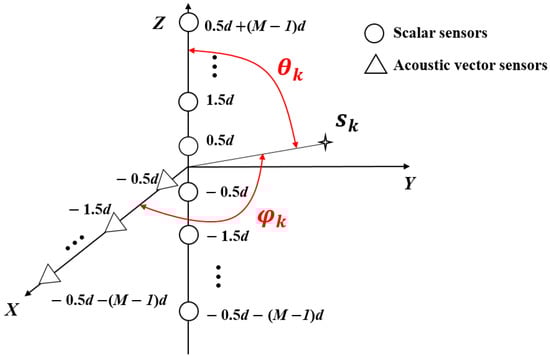
Figure 1.
Proposed hybrid T-shaped sensor array configuration.
The received signal vector of Z-ULA and matrix of X-ULA from K sources at the nth snapshot can be represented as
where and are temporally and spatially Gaussian white with zero-mean additive noise vector and matrix corresponding to the Z-ULA and X-ULA, respectively, and is the spatial response vector of the acoustic vector sensor located at the origin. An acoustic vector sensor consists of an omnidirectional pressure sensor and up to three orthogonal particle velocity sensors, which can be expressed as [26]
3. Tensor Model for Hybrid T-Shaped Sensor Array
3.1. Virtual URA with Acoustic Vector Sensors
We begin by constructing a virtual URA with acoustic vector sensors from the cross-correlation tensor [27] of and , i.e.,
where . Since the noise is assumed to be spatially independent, and X-ULA and Z-ULA have no common array elements, the cross-correlation tensor no longer contains the terms related to noise.
According to , we reverse the order of the lateral slices [27] of the tensor , and we obtain a new tensor
where . Moreover, since and are the same in data Equation (3), the can be directly written as . Obviously, can be considered as the received data tensor of a virtual URA with acoustic vector sensors, where and are the steering vectors for the kth source along the z and x axes, respectively, and is the spatial response vector of the acoustic vector sensor located at the origin of the kth source.
Therefore, tensor can correspond to a (virtual) URA of 2M2 acoustic vector sensors which lies in the left half of the XZ plane, as depicted in Figure 2.
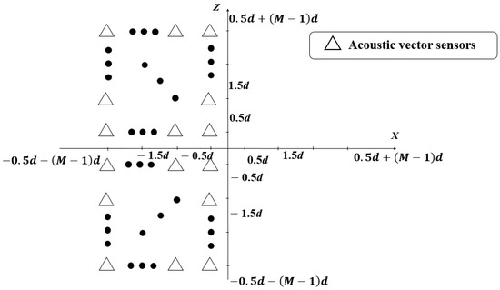
Figure 2.
Virtual URA with Acoustic Vector Sensors in the left half of the XZ plane.
To obtain another virtual URA, we calculate the conjugate tensor of firstly, i.e.,
According to , we reverse the order of the horizontal slices [21] of , and then we can obtain a new tensor
Similarly, can be considered as the received data tensor of another virtual URA of 2M2 acoustic vector sensors, which lies in the right half of the XZ plane, as shown in Figure 3.
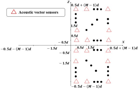
Figure 3.
Virtual URA with Acoustic Vector Sensors in the right half of the XZ plane.
Note that and have the same dimensions (i.e., and ), so we can combine them into a larger one. Let be the tensor of size , which is given by
and then the tensor can be described as
where and .
Similar to Equations (5) and (7), tensor corresponds to a larger virtual URA, which contains all the acoustic vector sensors in the XZ plane as depicted in Figure 4. In addition, the element spacing of this larger virtual URA is d, which depends on the inter-sensor spacing of the physical T-shaped array.
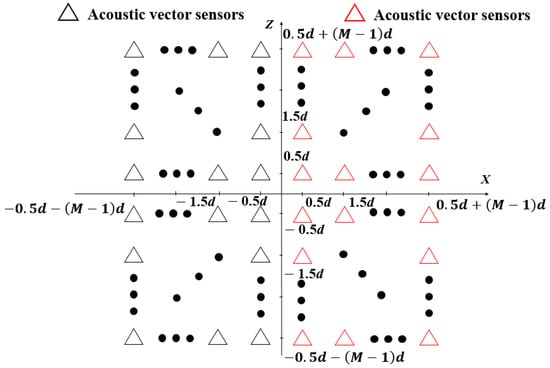
Figure 4.
Virtual URA with Acoustic Vector Sensors in XZ plane.
3.2. Maximization of DOF
Consider as a tensor of size ; then, behaves like the equivalent single-snapshot signals of the virtual URA. To increase the number of resolvable sources of the virtual URA, i.e., the DOF of the virtual URA, we increase the number of equivalent snapshots of by applying the spatial smoothing method [6]. It is worth noting that each sensor in our virtual URA is an acoustic vector sensor, while the one in [6] is a scalar sensor. Therefore, we utilize tensor algebra to achieve spatial smoothing.
Let us divide the virtual URA into overlapping identical subarrays of size . Note that and . Then, the received signal at the (nz, nx)th () subarray in the virtual URA can be given by
where and .
From Equation (11), we can see that has a Vandermonde structure. Therefore, let be the tensor of size , which is given by
and then can be expressed as
where and .
Via Definition 1 in [13], one can combine the second and fourth dimensions of to construct the dimension corresponding to equivalent snapshots, i.e.,
where .
To further increase the DOF, we combine the first and second dimensions of , i.e.,
where is the steering vector of our virtual URA.
From Equation (15), we can see that corresponds to a URA with acoustic vector sensors and contains equivalent snapshots.
From , the 2-D DOA estimation of the URA can be accomplished by the Vandermonde recovery of the factor matrix. Even so, the 2-D DOA estimation via a simpler method is recommended. Therefore, once the 2-D DOA estimation is achieved by the methods mentioned in the following text, the complex calculations of Vandermonde recovery can be avoided. Similar to [13,28], in order to easily calculate the DOA of the incident signals, we use the Vandermonde structure of to rearrange as a seventh-order tensor:
where and ; and .
We combine the dimensions of the seventh-order tensor as follows:
where and .
Finally, is the fourth-order canonical polyadic (CP) tensor model for our virtual URA.
Let represent Kruskal’s rank [27] of the matrix , and then our tensor model is sufficiently unique if [27]
where , , , and .
We assume that the DOA pairs are chosen by the condition given by [6], which guarantees , , , and . Then, applying the Lagrange multiplier method to Equation (18), we can find that when , the maximum number of identifiable sources for the proposed method is obtained, i.e.,
Remark 1.
For the proposed hybrid T-shaped sensor array composed of M acoustic vector sensors and 2M scalar sensors, we have established a fourth-order tensorto process its received signals, which corresponds to a URA with M2 acoustic vector sensors and contains (M + 1)2 equivalent snapshots. Thus, this virtual URA has M2 + 1 DOFs.
3.3. Two-Dimensional Angle Estimation via an Extended-Aperture Hybrid T-Shaped Sensor Array
According to the proposed tensor model , DOA information exists in different dimensions of the tensor. Utilizing the cp4_alsls MATLAB function [29] to carry out the CP tensor decomposition for , one can obtain the estimations of and , i.e., and .
According to , DOA estimates can be obtained from as follows:
where denotes returning the phase angle in the interval [−π,π] for each element of a complex array z. and are the cosine estimations of azimuth and elevation, respectively.
According to Equation (3), DOA estimates can also be obtained from as follows:
On the one hand, compared with and inherently extracted from information based on a single vector hydrophone which has no effective geometric aperture, and are extracted from information that encompasses the entire virtual array aperture and elements. Therefore, the estimates from have higher accuracy [15].
On the other hand, when the inter-sensor spacing of our array is set to be multiple half-wavelengths, there is a set of DOA estimates with cyclic ambiguity [30]. Assume a single source is impinging on the array from 2-D DOA . The phase differences between the received signals at two adjacent sensors in the x-direction and z-direction are respectively denoted as
where the mod operation is based on the principle that the phase of a signal rotates for every distance the signal travels. Hence the relationship between the phase difference and inter-element spacing is that
Since and , the above ranges for the two integers and are simplistically given according to their constraints and . For particular phase differences and , there exists one or a set of angles that satisfies Equation (25).
Specifically, when , both and can only take the value 0, which means that the azimuth angle and elevation angle have a one-to-one correspondence with cosine values within the range of 0 to . As increases, the numbers of possible and values increase. Thus, all possible values of and exist in two sets and in the azimuth and elevation angles of the kth signal that satisfy Equation (25).
Compared with and , and do not suffer any similar extended-aperture ambiguity regardless of the inter-sensor spacing [15]. It should be emphasized that based on the fourth-order model , we can simultaneously obtain these two sets of DOA estimates from different dimensions of the tensor. Thus, these two sets of estimates can be used for mutual disambiguation to yield a set of fine and unambiguous estimates without additional angle pairing, which is given by
where and are taken as the true estimates if obtains the minimum value. From the direction-cosine estimates derived above, the kth signal’s azimuth and elevation arrival angles may be estimated as
The overall procedure of the proposed algorithm is summarized in Algorithm 1.
Remark 2.
As in [15,16,21], the inter-sensor spacing in our array can also be allowed to exceed a half-wavelength greatly to extend the array aperture, while our method has a much higher DOF than others. As in [10,12,13], the proposed method can also provide a much higher DOF than the number of physical sensors, while only our array is able to enlarge the inter-sensor spacing to extend the array aperture. Accordingly, the proposed method can simultaneously offer high DOF and large array aperture.
| Algorithm 1. Summary of the proposed algorithm. |
| Input: and of the Equations (1) and (2) in Equations (4) and (6) , and build Maximize DOF for from Equations (11) to (17) and build Conduct CP decomposition on and obtain two sets of DOA estimation from and Resolve cyclic ambiguity to obtain accurate estimates. |
4. Numerical Simulation
To prove that our array can achieve better performance under the same array cost, we compare it with the vector sensor arrays of large array aperture [15,16,21]. In addition, since our array contains scalar sensors, some scalar arrays with high DOFs [10,12,13] are used as benchmarks. All the simulation results are obtained via 100 Monte Carlo trials. The root mean square error (RMSE) of parameter estimation is defined as
where and are the estimations of elevation angle and azimuth angle in the jth experiment for the kth signal and is the number of Monte Carlo trials.
4.1. Identifiability of the Proposed Method
We consider the hybrid T-shaped sensor array with 6 acoustic vector sensors and 12 scalar sensors. The snapshot number N, and signal-to-noise ratio (SNR) are set to be 500 and 10 dB, respectively. The sensor spacing of the proposed method . The 36 narrow-band waves impinge on the array, whose DOAs are chosen by 36 pairs as {(52 + m1(74 − 52)/7, 52 + m2(74 − 52)/7), m1 = 1, …,6, m2 = 1, …,6} according to the condition given by [6]. It can be seen from the estimated results shown in Figure 5 that the proposed method can effectively handle the 36 sources which are more than 18 array elements.
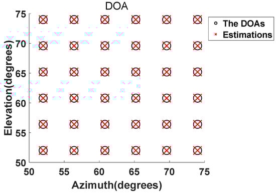
Figure 5.
Estimations of 36 sources.
4.2. RMSE vs. SNR
This example investigates the processing performance of the proposed method concerning SNR. In the proposed method, we utilize 6 acoustic vector sensors (containing 24 sensor components) and 12 scalar sensors. For the purpose of comparison, we consider scalar sensors as a component of vector sensors. Now, this proposed array contains 36 sensor components. Therefore, 36 vector sensor components are used in [15,16,21], under the same array cost. The SNR is varied from −5 dB to 20 dB. The azimuth and elevation angles of the two sources are set to (46°, 55°) and (48°, 62°), respectively. The snapshot number is set to 500. References [15,16,21] can allow 100× half-wavelength spacing, but the graph is constructed setting this to only 5×, i.e., d = 5 × (λ/2). The inter-sensor spacing of other methods is set to be (λ/2). From the results in Figure 6, we can see that [15,16,21] have better performance than [10,12,31] due to the array aperture advantage. Note that although the method in [13] utilizes the scalar sensor array needing at least one inter-sensor spacing not larger than half a wavelength, it can achieve a much higher DOF than [15,16,21]. Therefore [13] also shows better performance. The proposed method can simultaneously offer DOF as in [13] and large array aperture as in [15,16,21]. Accordingly, the proposed method has the smallest RMSE among all considered methods.
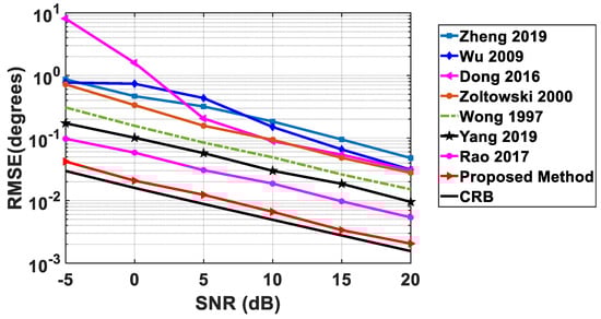
Figure 6.
RMSE versus SNR.
4.3. RMSE vs. N
In this example, we examine the performance of the proposed method against the number of snapshots N. N is varied from 100 to 800, and SNR is fixed at 10 dB, while the other parameters are the same as in the second example. From the results shown in Figure 7, we can see that for all cases, the proposed method yields the best estimation results.
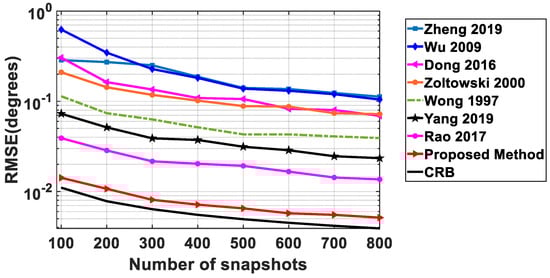
Figure 7.
RMSE versus N.
4.4. Runtime vs. the Number of Sensor Components
In this experiment, we compared the runtime required for each algorithm to run once in MATLAB 2022b on the same computer. The results are shown in Figure 8. For the purpose of comparison, we consider scalar sensors as a component of vector sensors. Other conditions are the same as Experiment 2, except that the total number of sensor components changes from 24 to 72. From Figure 6, it can be seen that the running time of the proposed method increases with an increase in the total number of sensor components. This is because the larger the number of sensor components is, the larger the size of is, resulting in more time being needed to achieve the tensor decomposition. However, it is important to note that the larger size of also means a higher DOF. Compared with other faster algorithms, although our algorithm may not be the most computationally efficient, it nonetheless belongs to the class of algorithms with relatively low computational complexity.
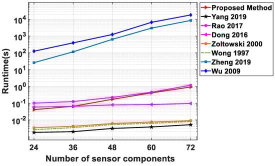
Figure 8.
Runtime versus the number of sensor components.
5. Conclusions
To reduce the cost of the 2-D vector sensor array, a new hybrid T-shaped sensor array composed of acoustic vector sensors and scalar sensors has been proposed. The tensor-based approach to this array processing with enhanced DOF and extended array aperture has been provided. Specifically, the proposed array contains M acoustic vector sensors and 2M scalar sensors, which are respectively placed along the x-axis and z-axis. Utilizing the cross-correlation tensor of the array received signals, a data tensor corresponding to a virtual URA with acoustic vector sensors is constructed. Applying the conjugate symmetry property of the ULA manifold matrix to the cross-correlation tensor, the data tensor of another virtual URA with acoustic vector sensors is also constructed. The analysis shows that these two virtual URAs can be combined into a larger virtual URA with 4M2 acoustic vector sensors. It is shown that a virtual URA with approximately M2 + 1 DOFs can be obtained. Since all the array elements in the virtual URA are acoustic vector sensors, the inter-sensor spacing can be extended with the help of the acoustic vector sensor characteristics. Thus, the proposed method has both a higher DOF and a larger array aperture. As demonstrated by simulation results, the proposed method can achieve superior 2-D DOA estimation performance to many existing methods under the same array cost. Additionally, 2-D DOA estimation is achieved by the CP decomposition, which means the multidimensional search can be avoided.
The hybrid concept proposed herein may be applied to other types of sensors, such as electromagnetic vector sensors, for highly accurate angle estimation with increased DOF and array aperture. Naturally, it can also be applied to other types of nonuniform arrays, such as nested arrays, coprime arrays, and minimum redundancy arrays.
Author Contributions
Conceptualization, W.R.; methodology, W.R.; software, Y.L.; validation, W.R.; formal analysis, W.R.; writing—original draft preparation, Y.L.; writing—review and editing, W.R.; supervision, W.R. and D.L.; All authors have read and agreed to the published version of the manuscript.
Funding
This work was supported in part by the National Natural Science Foundation of China under Grant 61961025 and in part by the Jiangxi Provincial Natural Science Foundation under Grant 20202BABL202001.
Data Availability Statement
Data sharing is not applicable.
Conflicts of Interest
The authors declare no conflict of interest.
References
- Krim, H.; Viberg, M. Two decades of array signal processing research: The parametric approach. IEEE Signal Process. Mag. 1996, 13, 67–94. [Google Scholar] [CrossRef]
- Zheng, Z.; Fu, M.; Wang, W.-Q.; Zhang, S.; Liao, Y. Localization of mixed near-field and far-field sources using symmetric double-nested arrays. IEEE Trans. Antennas Propag. 2019, 67, 7059–7070. [Google Scholar] [CrossRef]
- Wang, X.; Wan, L.; Huang, M.; Shen, C.; Han, Z.; Zhu, T. Low-complexity channel estimation for circular and noncircular signals in virtual MIMO vehicle communication systems. IEEE Trans. Veh. Technol. 2020, 69, 3916–3928. [Google Scholar] [CrossRef]
- He, W.; Yang, X.; Wang, Y. A high-resolution and low-complexity DOA estimation method with unfolded coprime linear arrays. Sensors 2019, 20, 218. [Google Scholar] [CrossRef] [PubMed]
- Aboumahmoud, I.; Muqaibel, A.H.; Alhassoun, M.; Alawsh, S.A. A Review of Sparse Sensor Arrays for Two-Dimensional Direction-of-Arrival Estimation. IEEE Access 2021, 9, 92999–93017. [Google Scholar] [CrossRef]
- Pal, P.; Vaidyanathan, P. Nested arrays in two dimensions, part II: Application in two dimensional array processing. IEEE Trans. Signal Process. 2012, 60, 4706–4718. [Google Scholar] [CrossRef]
- Vaidyanathan, P.P.; Pal, P. Sparse sensing with co-prime samplers and arrays. IEEE Trans. Signal Process. 2010, 59, 573–586. [Google Scholar] [CrossRef]
- Qin, S.; Zhang, Y.D.; Amin, M.G. Two-dimensional DOA estimation using parallel coprime subarrays. In Proceedings of the 2016 IEEE Sensor Array and Multichannel Signal Processing Workshop (SAM), Rio de Janeiro, Brazil, 10–13 July 2016; pp. 1–4. [Google Scholar]
- Zheng, W.; Zhang, X.; Zhai, H. Generalized coprime planar array geometry for 2-D DOA estimation. IEEE Commun. Lett. 2017, 21, 1075–1078. [Google Scholar] [CrossRef]
- Zheng, Z.; Mu, S. Two-dimensional DOA estimation using two parallel nested arrays. IEEE Commun. Lett. 2019, 24, 568–571. [Google Scholar] [CrossRef]
- Si, W.; Zeng, F.; Qu, Z.; Peng, Z. Two-dimensional DOA estimation via a novel sparse array consisting of coprime and nested subarrays. IEEE Commun. Lett. 2020, 24, 1266–1270. [Google Scholar] [CrossRef]
- Dong, Y.-Y.; Dong, C.-X.; Liu, W.; Chen, H.; Zhao, G.-q. 2-D DOA estimation for L-shaped array with array aperture and snapshots extension techniques. IEEE Signal Process. Lett. 2017, 24, 495–499. [Google Scholar] [CrossRef]
- Rao, W.; Li, D.; Zhang, J.Q. A tensor-based approach to L-shaped arrays processing with enhanced degrees of freedom. IEEE Signal Process. Lett. 2017, 25, 1–5. [Google Scholar] [CrossRef]
- Zheng, H.; Shi, Z.; Zhou, C.; Haardt, M.; Chen, J. Coupled Coarray Tensor CPD for DOA Estimation With Coprime L-Shaped Array. IEEE Signal Process. Lett. 2021, 28, 1545–1549. [Google Scholar] [CrossRef]
- Wong, K.T.; Zoltowski, M.D. Extended-aperture underwater acoustic multisource azimuth/elevation direction-finding using uniformly but sparsely spaced vector hydrophones. IEEE J. Ocean. Eng. 1997, 22, 659–672. [Google Scholar] [CrossRef]
- Zoltowski, M.D.; Wong, K.T. ESPRIT-based 2-D direction finding with a sparse uniform array of electromagnetic vector sensors. IEEE Trans. Signal Process. 2000, 48, 2195–2204. [Google Scholar] [CrossRef]
- Yang, M.; Ding, J.; Chen, B.; Yuan, X. A multiscale sparse array of spatially spread electromagnetic-vector-sensors for direction finding and polarization estimation. IEEE Access 2018, 6, 9807–9818. [Google Scholar] [CrossRef]
- He, J.; Zhang, Z.; Shu, T.; Yu, W. Sparse nested array with aperture extension for high accuracy angle estimation. Signal Process. 2020, 176, 107700. [Google Scholar] [CrossRef]
- Liu, S.; Zhao, J.; Zhang, Y.; Wu, D. 2D DOA Estimation Algorithm by Nested Acoustic Vector-Sensor Array. Circuits Syst. Signal Process. 2021, 41, 1115–1130. [Google Scholar] [CrossRef]
- He, J.; Li, L.; Shu, T. Sparse nested arrays with spatially spread square acoustic vector sensors for high-accuracy underdetermined direction finding. IEEE Trans. Aerosp. Electron. Syst. 2021, 57, 2324–2336. [Google Scholar] [CrossRef]
- Yang, M.; Ding, J.; Chen, B.; Yuan, X. Coprime L-shaped array connected by a triangular spatially-spread electromagnetic-vector-sensor for two-dimensional direction of arrival estimation. IET Radar Sonar Navig. 2019, 13, 1609–1615. [Google Scholar] [CrossRef]
- Fu, M.; Zheng, Z.; Wang, W.-Q.; So, H.C. Coarray interpolation for DOA estimation using coprime EMVS array. IEEE Signal Process. Lett. 2021, 28, 548–552. [Google Scholar] [CrossRef]
- Qu, X.; Lou, Y.; Zhao, Y.; Lu, Y.; Qiao, G. Augmented Tensor MUSIC for DOA Estimation Using Nested Acoustic Vector-Sensor Array. IEEE Signal Process. Lett. 2022, 29, 1624–1628. [Google Scholar] [CrossRef]
- Cao, J.; Liu, J.; Wang, J.; Lai, X. Acoustic vector sensor: Reviews and future perspectives. IET Signal Process. 2017, 11, 1–9. [Google Scholar] [CrossRef]
- Rahamim, D.; Tabrikian, J.; Shavit, R. Source localization using vector sensor array in a multipath environment. IEEE Trans. Signal Process. 2004, 52, 3096–3103. [Google Scholar] [CrossRef]
- Nehorai, A.; Paldi, E. Acoustic vector-sensor array processing. IEEE Trans. Signal Process. 1994, 42, 2481–2491. [Google Scholar] [CrossRef]
- Kolda, T.G.; Bader, B.W. Tensor decompositions and applications. SIAM Rev. 2009, 51, 455–500. [Google Scholar] [CrossRef]
- Sidiropoulos, N.D. Generalizing Caratheodory’s uniqueness of harmonic parameterization to N dimensions. IEEE Trans. Inf. Theory 2001, 47, 1687–1690. [Google Scholar] [CrossRef]
- Vervliet, N.; Debals, O.; De Lathauwer, L. Tensorlab 3.0—Numerical optimization strategies for large-scale constrained and coupled matrix/tensor factorization. In Proceedings of the 2016 50th Asilomar Conference on Signals, Systems and Computers, Pacific Grove, CA, USA, 6–9 November 2016; pp. 1733–1738. [Google Scholar]
- Wu, Q.; Sun, F.; Lan, P.; Ding, G.; Zhang, X. Two-dimensional direction-of-arrival estimation for co-prime planar arrays: A partial spectral search approach. IEEE Sens. J. 2016, 16, 5660–5670. [Google Scholar] [CrossRef]
- Kawitkar, R. Performance of different types of array structures based on multiple signal classification (MUSIC) algorithm. In Proceedings of the 2009 5th International Conference on MEMS NANO, and Smart Systems, Dubai, United Arab Emirates, 28–30 December 2009; pp. 159–161. [Google Scholar]


Disclaimer/Publisher’s Note: The statements, opinions and data contained in all publications are solely those of the individual author(s) and contributor(s) and not of MDPI and/or the editor(s). MDPI and/or the editor(s) disclaim responsibility for any injury to people or property resulting from any ideas, methods, instructions or products referred to in the content. |
© 2023 by the authors. Licensee MDPI, Basel, Switzerland. This article is an open access article distributed under the terms and conditions of the Creative Commons Attribution (CC BY) license (https://creativecommons.org/licenses/by/4.0/).