A Novel AB-CNN Model for Multi-Classification Sentiment Analysis of e-Commerce Comments

Abstract

Despite the success of dichotomous sentiment analysis, it does not encompass the various emotional colors of users in reality, which can be more plentiful than a mere positive or negative association. Moreover, the complexity and imbalanced nature of Chinese text presents a formidable obstacle to overcome. To address prior inadequacies, the three-classification method is employed and a novel AB-CNN model is proposed, incorporating an attention mechanism, BiLSTM, and a CNN. The proposed model was tested on a public e-commerce dataset and demonstrated a superior performance compared to existing classifiers. It utilizes a word vector model to extract features from sentences and vectorize them. The attention layer is used to calculate the weighted average attention of each text, and the relevant representation is obtained. BiLSTM is then employed to read the text information from both directions, further enhancing the emotional level. Finally, softmax is used to classify the emotional polarity.

1. Introduction

Sentiment analysis, also known as sentiment tendency analysis or opinion mining, is the process of extracting information from user opinions [1]. It involves obtaining people’s attitudes, emotions, and opinions through the analysis of text, audio, and images. Sentiment analysis is the process of analyzing, processing, and interpreting text with emotion. The Internet has seen an influx of texts with emotional sentiment, prompting researchers to move from the initial analysis of emotional words to more complex analysis of emotional sentences and articles. As a result, the fine-grained processing of text varies, and sentiment analysis can be divided into three levels: word-level, sentence-level, and chapter-level research [2]. Sentiment analysis can be divided into two categories: analysis of social platform reviews and analysis of e-commerce platform reviews. The former mainly focuses on social platform reviews, while the latter focuses on product reviews from e-commerce platforms. For instance, a positive review such as “This phone is cost-effective and runs smoothly” indicates that the consumer is satisfied with the product. A neutral review such as “The overall feel of the phone is so-so!” implies that the consumer still approves of the product. On the other hand, a negative review such as “This phone is rubbish, a real card!” implies that the consumer is not satisfied with the product. Sentiment analysis of e-commerce reviews helps consumers quickly understand the public opinion of a certain product, making it popular among consumers and e-commerce websites. Meanwhile, sentiment analysis of social platform reviews is mostly used for public opinion monitoring and information prediction.

This paper focuses on sentiment analysis of comments on e-commerce platforms, categorizing ratings into three classes: negative (one and two stars), neutral (three stars), and positive (four and five stars). We then load the e-commerce review dataset into a trained deep-learning model for research and analysis. Our method combines an attention mechanism, BiLSTM, and a CNN to create an AB-CNN-based model and perform classification prediction.

The following sections of this article will be discussed: Section 2: analysis of previous related studies; Section 3: overview of relevant theories; Section 4: presentation of the paper’s model and brief introduction; Section 5: experimentation and analysis of results; Section 6: conclusions and summary.

2. Related Work

Sentiment analysis of texts has been a popular research topic since the introduction of emotional dictionaries, through to traditional machine learning and now deep learning. Research in this field primarily centers on emotional dictionaries, machine learning, and deep learning.

2.1. The Emotional-Dictionary-Based Methods

Sentiment analysis based on sentiment dictionaries involves obtaining the emotional value of a sentence in a text, and then determining the text’s emotional tendency through weighted calculation. For example, Zargari H et al. [3] proposed an N-Gram sentiment dictionary method based on global intensifiers, which increases the coverage of emotion phrases in the dictionary. Yan et al. [4] constructed a comprehensive dictionary of emotional polarity through artificial annotation, including basic, negative, adverbial degree, and flip dictionaries, to enhance the accuracy of sentiment analysis. Wang et al. [5] proposed an enhanced NTU sentiment dictionary, which was constructed by collecting sentiment statistics of words in several sentiment annotation works, and provided rich semantic information. Its application in the polarity classification of words has achieved good results. Zhang et al. [6] trained Weibo texts based on adverbial, network, and negative dictionaries to obtain updated sentiment values. Based on the existing sentiment lexicon, Jia K et al. [7] improved the calculation method of the sentiment intensity of the sentiment words of different sentiment categories in the sentiment lexicon. By combining sentiment lexicon and semantic rules, the sentiment intensity of micro-blogs with different sentiment categories is calculated and sentiment classification is realized. Xu et al. [8] established an extended emotional lexicon comprising basic, scene, and polysomic emotional words, which further improved the emotional classification effect of texts. Phan T et al. [9] proposed a sentiment dictionary for Vietnamese, containing over 100,000 Vietnamese emotional words. Wei Wang et al. [10] proposed a U-shaped acoustic word sentiment lexicon feature model based on AWED. This method can be used to build an emotional information model from the acoustic vocabulary level of different emotional categories. The results show that the proposed method achieves significant improvements in unweighted average recall in all four sentiment classification tasks.

2.2. The Machine-Learning-Based Methods

Sentiment analysis using machine learning involves leveraging traditional machine learning algorithms to extract features from labeled or unlabeled datasets and then producing sentiment analysis results. For instance, Guanghan M [11] proposed a micro-blog emotion-mining method based on word2vec and a support vector machine (SVM). This method weighted the trained word vectors of word2vec and calculated different expected word frequencies, followed by sentiment analysis in SVM. Xue et al. [12] constructed a data sentiment classifier based on the Naive Bayes principle and analyzed the sentiment tendency of the tested text with the constructed sentiment classifier. Wawre et al. [13] compared SVM and Naive Bayes (NB) machine learning methods and found that NB had a higher classification accuracy than SVM for large datasets. Kamal et al. [14] proposed a rule-based and machine learning combination method to identify its emotional polarity, achieving good results. Rathor et al. [15] compared and analyzed SVM, NB, and ME machine learning algorithms using weighted letters, and the results show that all three algorithms achieved good classification effects. Zhang et al. [16] proposed an AE-SVM algorithm and achieved satisfactory results when applied to the employee sentiment analysis dataset of company evaluation. Mitroi, M. et al. [17] proposed novel topical document embedding (TOPICDOC2VEC) to detect the polarity of text. TOPICDOC2VEC is constructed as a connection between document embeddings (DOC2VEC) and topic embeddings (TOPIC2VEC), and experimental results show that TOPICDOC2VEC embeddings outperform DOC2VEC embeddings in detecting document polarity.

2.3. The Deep-Learning-Based Methods

Deep learning has achieved remarkable success in the field of image processing, leading to an increased interest in sentiment analysis based on this technology. Current deep learning models include CNNs, LSTM, BiLSTM, RNNs, and attention mechanisms. For instance, Teng et al. [18] proposed a topic classification model based on LSTM, which is capable of processing vector, array, and high-dimensional data. Yin et al. [19] used a BiGRU neural network layer for feature enhancement, achieving this through superposition and reuse, and faster convergence through continuous enhancement. This network outperformed other classification models. He et al. [20] extracted word-embedding and sequence features from the word vector based on vocabulary, fused the two features into SVM input, and finally determined the emotional polarity of the text. Zeng et al. [21] proposed the PosATT-LSTM model, which takes into account the significance of the connection between context words and context location. Zhou et al. [22] proposed a Chinese sentiment analysis method that combined word2vec and Stacked BiLSTM, resulting in improved performance. Su et al. [23] proposed an AEB-CNN model incorporating emoji attention and a CNN, which enhanced the accuracy of sentiment analysis. Truică, Ciprian-Octavian et al. [24] proposed a new document-topic-embedding model for document-level polarity detection in large texts by using general and specific contextual cues obtained from document embedding (DOC2VEC) and topic modeling and achieved promising results. Petrescu, Alexandru et al. [25] proposed a new ensemble architecture, EDSA-Ensemble (Event Detection Sentiment Analysis Ensemble), which uses event detection and sentiment analysis to improve polarity detection of current events from social media. The ensemble model has achieved good results in deep learning and machine learning.

3. Related Theory

3.1. Attention Mechanism

Treisman [26] proposed in 1980 that deep learning’s mechanism of attention borrows from the way human vision operates. Physiologically, when humans observe their environment, they quickly scan the panorama and, based on brain signals, quickly focus their attention on the target area, forming a focus of attention to obtain more details and suppress irrelevant information.

When using NLP for text tasks, the attention mechanism can be employed to prioritize the text content that requires attention, thus increasing the model’s running speed, reducing complexity, shortening training time, and improving prediction accuracy. In sentiment analysis, the attention layer on the CNN is used to focus on words or sentences related to emotions, discarding other text information that is not emotionally relevant.

Given an input text sequence $X$, a query vector $q$ is used to identify important information. The query process is conducted across $X$, with each word contributing its own attention, and words with emotional color contributing more.

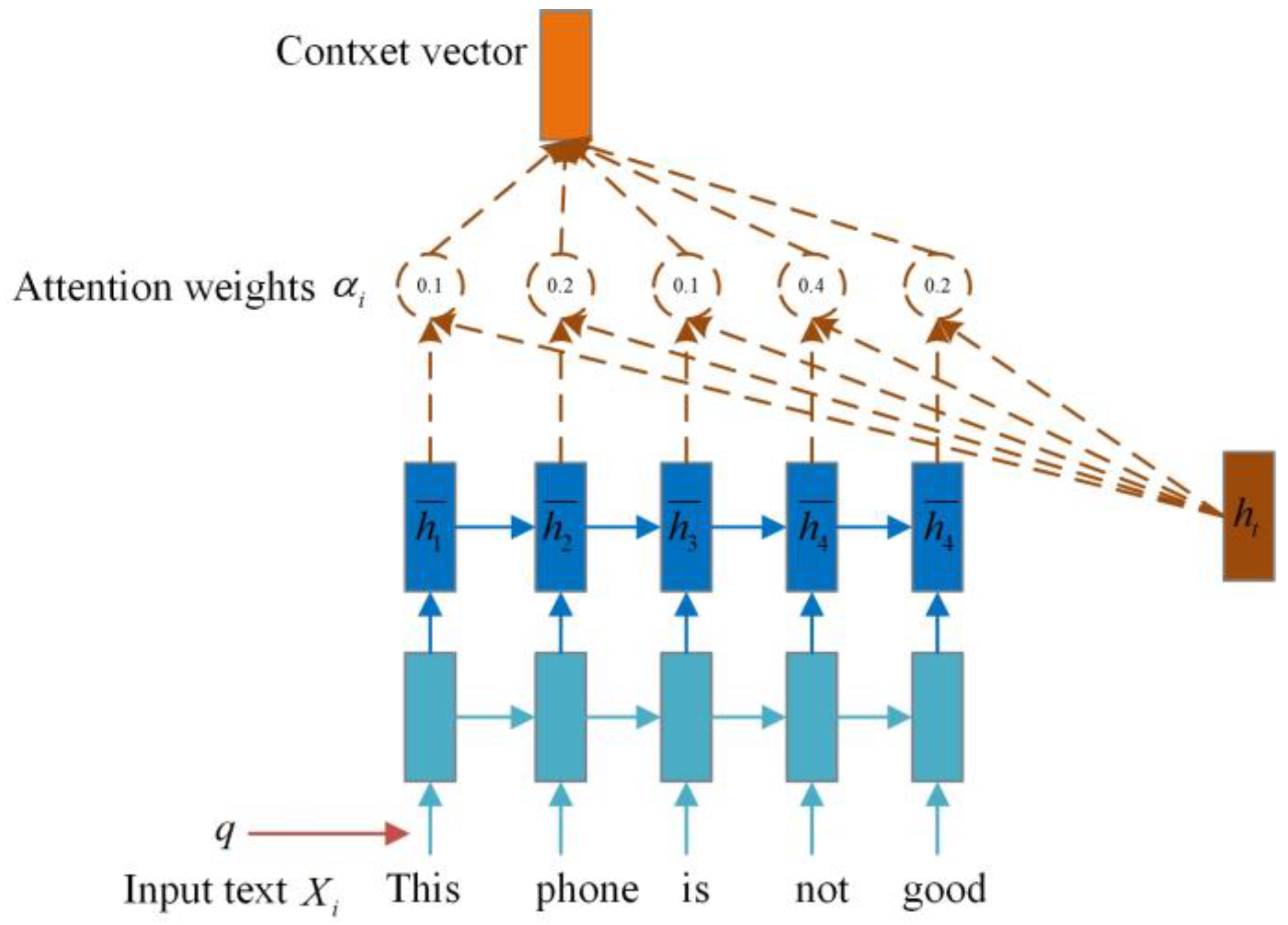
To reduce complexity, an attention variable $U\in \left[1,N\right]$ is defined to represent the index of the selected query information. Figure 1 illustrates the calculation process, which is the manifestation of the attention mechanism. This allows only emotion-related words or sentences to be selected from $X$ and inputted into the model for training, instead of all the text information content.

Figure 1. The computational process of the attention mechanism.

The attention mechanism consists of three steps: text input, calculation of the attention weight coefficient$\alpha$, and weighted average of input information.

• Text information input: $X=\left[X_1,X_2,\dots ,X_N\right]$ represents$N$ input text information content.
• The attention weight between the $i$th word and $q$ is calculated using the formula Equation (1):

  $${\alpha }_i=P\left(U=i|X,q\right)=softmax\left(s\left(X_i,q\right)\right)$$

  (1)

${\alpha }_i$ is the weight coefficient of attention, and $s\left(X_i,q\right)$ is the calculation function. The main calculation methods include the following formulae, Equations (2)–(5):

$$\mathrm{Additive} \mathrm{model}: s\left(X_i,q\right)=V^{T}tanh\left(W{X}_i+U_q\right)$$

(2)

$$\mathrm{Dot} \mathrm{product} \mathrm{model}: s\left(X_i,q\right)=x_i^{T}q$$

(3)

$$\mathrm{Scaled} \mathrm{dot} \mathrm{product} \mathrm{model}: s\left(X_i,q\right)=\frac{X_i^{T}q}{\sqrt{d}}$$

(4)

$$\mathrm{Bilinear} \mathrm{model}: s\left(X_i,q\right)=X_i^{T}Wq$$

(5)

Let$W$,$U$, and $V$ be variables in the network model, where $d$denotes the latitude of the input word vector.

3.

The weight coefficient of attention ${\alpha }_i$, encodes the input text information $X$. The attention degree of the $i$th information concerning the context query vector $q$ is calculated using Equation (6):

$$attention\left(q,X\right)={\displaystyle \sum }_{i=1}^N{\alpha }_i{X}_i$$

(6)

3.2. BiLSTM

Long Short-Term Memory (LSTM) [27] is a type of Recurrent Neural Network (RNN) that has been found to suffer from issues such as gradient disappearance, gradient explosion, and a limited ability to read a range of information. To address these issues, LSTM was introduced, featuring the “memory time sequence” capability, allowing it to quickly learn the relationship between input text data and context.

Based on a basic RNN, LSTM enhances two aspects:

• New internal state:

LSTM introduces an internal state $c_t\in R^D$ and outputs information to the hidden layer’s external state $h_t\in R^D$. This internal state is calculated using Equations (7) and (8):

$$c_t=f_t⨀c_{t-1}+i_t⨀{\tilde{c}}_t$$

(7)

$$h_t=o_t⨀tanh\left(c_t\right)$$

(8)

The $f_t$,$i_t$,$o_t$ forms the path for the information to pass through, with the vector product of elements ⨀ and the memory unit of the moment ${\tilde{c}}_t\in R^D$ obtained using a nonlinear function candidate status. Equation (9) is as follows:

$${\tilde{c}}_t=tanh\left(W_c{x}_t+U_c{h}_{t-1}+b_c\right)$$

(9)

2.

Gating mechanism:

The LSTM network controls the flow of information through the implementation of three gating mechanisms: the forget gate $f_t$, the input gate $i_t$, and the output gate $o_t$. The values of these gates range from 0 to 1, indicating the proportion of text information that is allowed to pass through. Equations (10)–(12) are as follows:

$$f_t=\sigma \left(W_f{x}_t+U_f{h}_{t-1}+b_f\right)$$

(10)

$$i_t=\sigma \left(W_i{x}_t+U_i{h}_{t-1}+b_i\right)$$

(11)

$$o_t=\sigma \left(W_o{x}_t+U_o{h}_{t-1}+b_o\right)$$

(12)

Let $\sigma \left(·\right)$ denote the logistic function, $x_t$ the current input, and $h_{t-1}$ the external state of the preceding moment.

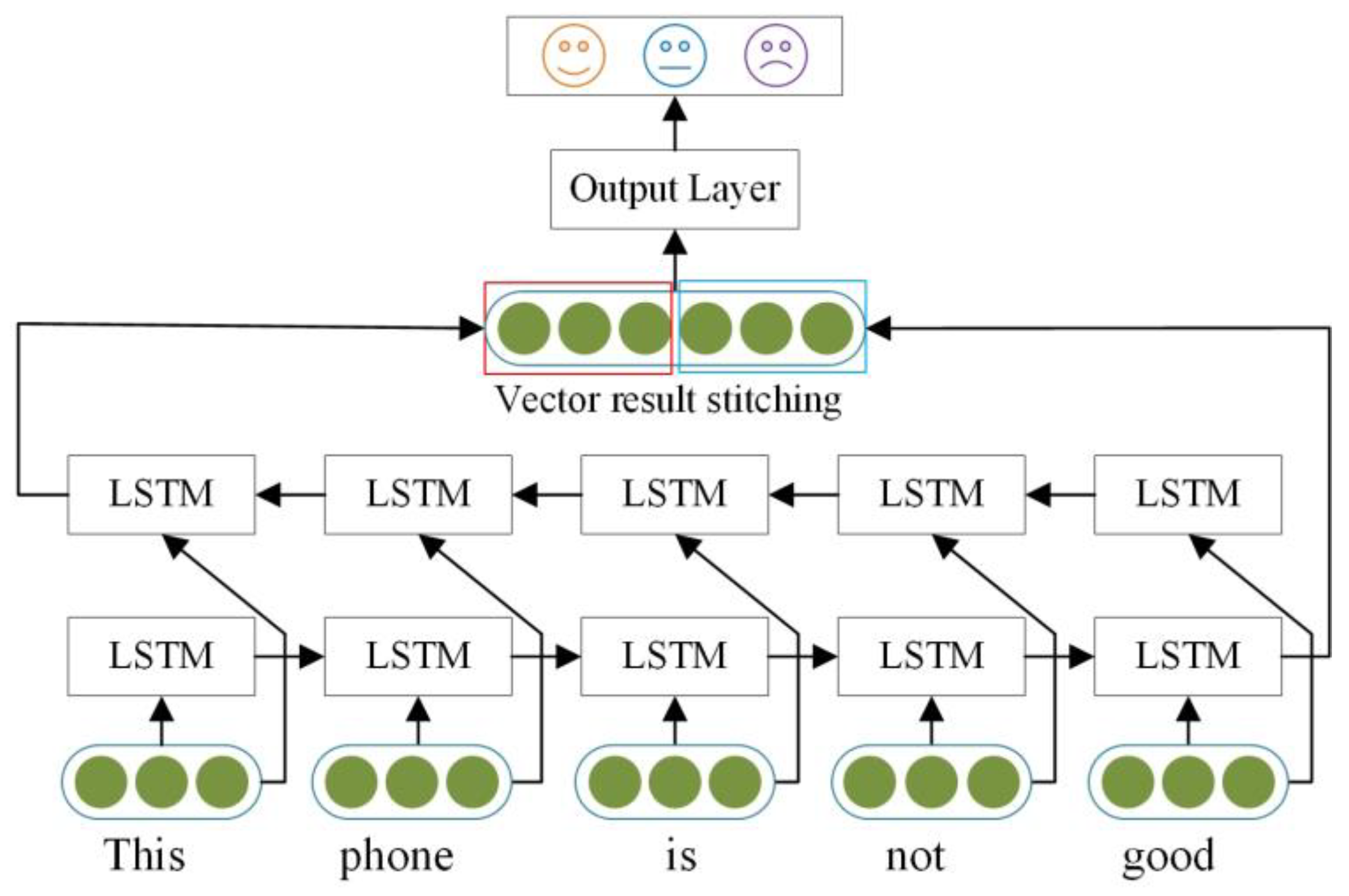
BiLSTM [28] divides an input sequence into two independent LSTMs, which process the sequence in both the forward and reverse directions to extract features. The final expression of the word is created by merging the output vectors of two LSTMs.

The structural characteristics of the BiLSTM model are illustrated in Figure 2. Its design concept involves the incorporation of both past and future information into the feature data obtained at the $t$ moment. The output of the forward LSTM layer at the $t$ moment is denoted as $\overrightarrow{h_t}$, while the output of the backward LSTM layer is $\overleftarrow{h_t}$. Experiments demonstrate that the BiLSTM model is more efficient and effective at text feature extraction than a single-LSTM structure model. Furthermore, BiLSTM consists of two LSTM parameters that share the same word-embedding vector list, but are otherwise independent.

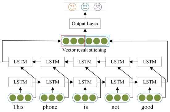
Figure 2. BiLSTM model structure.

3.3. CNN

Convolutional Neural Networks (CNNs) [29] have been widely adopted in the field of computer vision due to their high effectiveness. Starting with a convolutional layer, the network is further enhanced by the addition of layers such as pooling, dropout, and padding. Subsequently, GoogleNet, VGGNet, and ResNet, the most renowned CNNs in the field of image recognition, were developed, allowing neural networks to classify images with greater accuracy than humans. CNNs have efficient feature extraction and classification capabilities, which can be used to classify text information treated as a one-dimensional image, as illustrated in Figure 3.

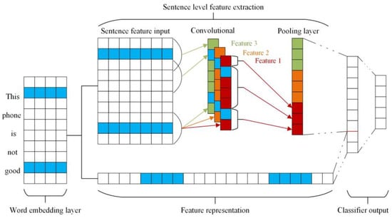
Figure 3. CNN text classification model.

The words in the input text are expressed as a matrix $X$, with each element $X_i$ representing a sequence vector in the word-embedding layer. This matrix is then used as the input of the CNN.

The features of the text are extracted by applying a sliding convolution with a kernel $k\in {ℝ}^{n\times d}$ on the original input text sequence. The $n-gram$ convolution is carried out using a sliding window scan with a step size of $s$, yielding $\left(N-n+1\right)$ features for each convolution kernel. A pooling layer is then used to select the text features with the highest weight, while ignoring the unimportant ones, thus obtaining the final word vector represented by the text features.

The pooling layer screens the text features, which are then connected to the predicted category labels. All text features are obtained, and the probability of each category label is calculated. The classification result is the maximum label probability value.

4. AB-CNN Model

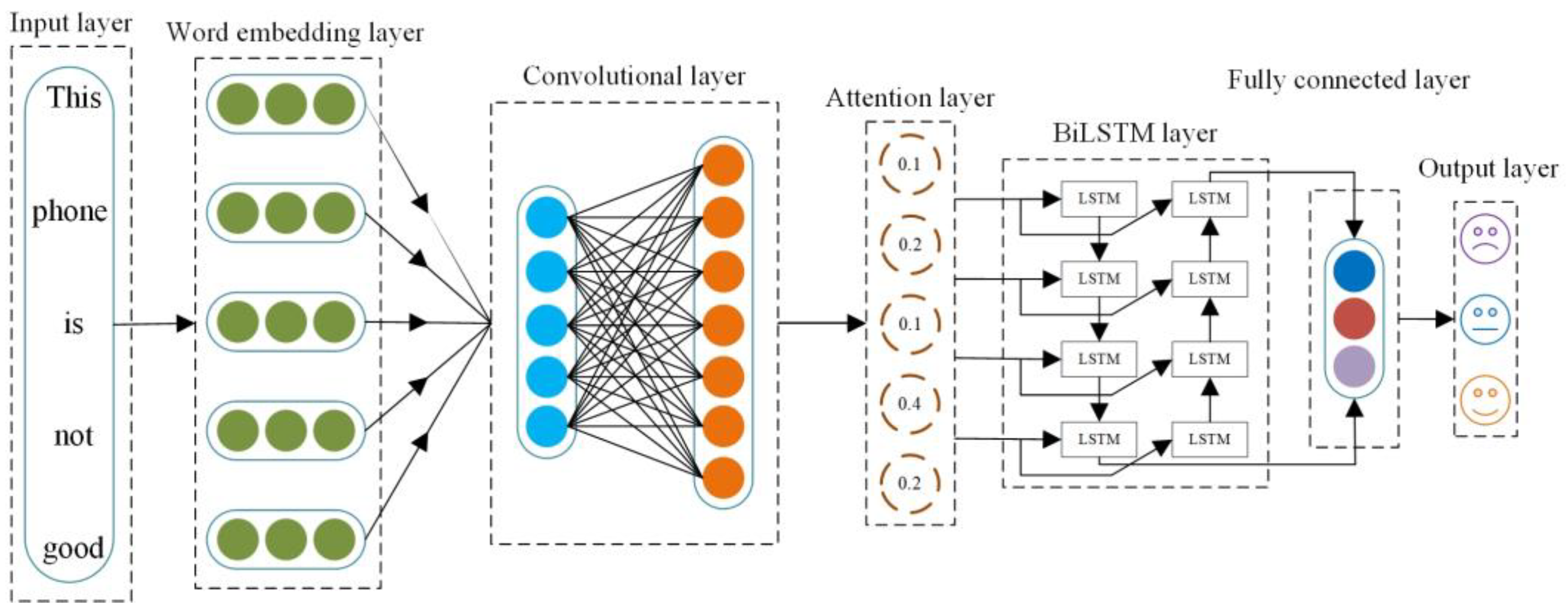
This paper’s model structure, comprising an input layer, word-embedding layer, convolutional layer, attention layer, BiLSTM layer, fully connected layer, and output layer, is depicted in Figure 4.

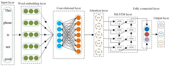
Figure 4. Structure of the AB-CNN model.

4.1. Word2vec Word-Vector-Embedding Layer

Let $m$ be a text composed of $n$ words, expressed as $m=\left[m_1,m_2,\cdots ,m_n\right]$. The input text sequence is converted to a word vector using word2vec, with an encoded latitude of 128, and initialized. The resulting vectorized form of the text is shown in Equation (13):

$$m_{1:n}=m_1\oplus m_2\oplus \cdots \oplus m_n$$

(13)

where $n$ denotes the length of each comment text sequence, with each word represented by a vector of$h$ dimensions and $m_i$ being the vector of the $i$th word in the sentence, connected by the operator $\oplus$.

The text sequence $m$ is segmented and converted into an $n\ast h$-dimensional vector matrix. This is then embedded into a low-dimensional word vector through an embedding layer, thus completing the conversion of text to a numerical vector.

4.2. CNN Layer

The output of the embedding layer is used as the convolutional layer input for the text sequence $m$. Applying $k$ convolutional filters $D=\left[{\phi }^1,{\phi }^2,\cdots ,{\phi }^k\right]$ with length $l$ to the $k\ast l$-dimensional word vector matrix of the $i$th word vector yields new features of the $i$th word of the text sequence $m$. Equation (14) is as follows:

$$n_i=f\left(D^T·m_{i:i+l-1}+b\right)$$

(14)

where $b\in ℝ$ is a bias term, $D^T$ the weight, and $f$ a nonlinear function $ReLu$. When the filter is applied to every word in the sentence $\left[m_{1:l},m_{2:l+1},\cdots ,m_{n-l+1:n}\right]$, the text characteristic expression is as follows, as shown in Equation (15):

$$N=\left[n_1,n_2,\cdots ,n_{n-l+1}\right]$$

(15)

Among them, $N\in {ℝ}^{n-l+1}$ uses the maximum pool operation, with the maximum value $\widehat{N}=max\left\{n\right\}$ as a filter characteristic. This ensures the most significant feature with the greatest value is acquired. The output of the convolutional layer is $Y$, and the equation is as follows, as shown in Equation (16):

$$Y=\left[N_1,N_2,\cdots ,N_{n-l+1}\right]$$

(16)

Then, the dropout layer is added after the convolutional layer to prevent over-fitting.

4.3. Attention Mechanism Layer

The convolutional layer can extract the important features of the text, while the attention layer can identify the words related to emotional polarity. This reduces the running time and complexity of the model. The attention mechanism is applied to the convolutional layer’s output $Y$, with a query vector $N_i$ for each text information input. The attention weight coefficient for each text feature $N_i$ can be calculated, the equation is as follows, as shown in Equation (17):

$${\alpha }_i=softmax\left(s\left(N_i,q\right)\right)=\frac{exp\left(s\left(N_i,q\right)\right)}{{{\displaystyle \sum }}_{j=1}^{n-l+1}exp\left(s\left(N_j,q\right)\right)}$$

(17)

Where $j$ is a parameter in the $softmax$ linear function, which means summing all text features $N_j$ and calculating the probability distribution of the $i$th text, namely the weight coefficient ${\alpha }_i$.

Where $i\in \left[1,2,\cdots ,n-l+1\right]$ is for the attention calculation function $s\left(N_i,q\right)$. You can choose the four models mentioned earlier for calculation.

After encoding the input text information $Y$ as follows, the weighted average attention signal of each text can be obtained. Equation (18) is shown as follows:

$$\overline{T}=attention\left(q,N\right)={\displaystyle \sum }_{i=1}^{n-l+1}{\alpha }_i{N}_i$$

(18)

Then, the attention signal $\overline{T}$ is mapped to the corresponding input text feature matrix $N_i$ to obtain a text matrix with an attention mechanism. This is expressed as $\overline{T}⨀N_i$.

Finally, after the attention is extracted through the convolution operation, the fusion of attention is carried out. Equation (19) is shown as follows:

$${\omega }_i={\mu }_1·N_i+{\mu }_2·N_i·\overline{T},i\in \left[1,2,\cdots ,n-l+1\right]$$

(19)

where ${\mu }_1$ is the weight of the original word vector, and ${\mu }_2$ is the weight of the attention signal. The word vector form after the integration of attention can be expressed as follows: $\omega =[{\omega }_1,{\omega }_2,\dots {\omega }_n]$.

4.4. BiLSTM Layer

The text word vector $\omega$ regarding emotional polarity is output by the attention layer as input to the BiLSTM layer. The two LSTMs integrate the input sequence’s information in both the forward and backward directions, thereby enhancing the emotional hue of the input text content and improving the model’s classification performance.

The forward LSTM layer of the output at the current moment has information from the current moment and the preceding one in the input sequence, while the backward LSTM layer has information from the current moment and the subsequent one in the input sequence.

The two LSTMs combine the input sequence’s information in both the forward and backward directions, splicing the word vectors to generate the BiLSTM result. This model can significantly enhance accuracy, with the forward output $\overrightarrow{h_t}$ and backward output $\overleftarrow{h_t}$at time $t$ shown in Equations (20) and (21):

$$\overrightarrow{h_t}=\overrightarrow{LSTM}\left(h_{t-1},{\omega }_t,c_{t-1}\right)$$

(20)

$$\overleftarrow{h_t}=\overleftarrow{LSTM}\left(h_{t-1},{\omega }_t,c_{t-1}\right)$$

(21)

Then, the BiLSTM output contains the emotional color $t$ moment, and the $i$th text feature vector is shown in Equation (22):

$$H_t^i=\left[\overrightarrow{h_t},\overleftarrow{{\mathrm{h}}_t}\right]$$

(22)

The output of the BiLSTM network’s text sequence semantic information extraction is $Q=\left[H_t^1,H_t^2,\cdots ,H_t^{n-l+1}\right]$.

4.5. Softmax Classification Output Layer

The input text is vectorized from the embedding layer using word2vec. The convolutional layer is then employed to classify and extract significant features. The attention layer is utilized to extract semantic features associated with emotion. Meanwhile, BiLSTM is employed to extract text context information to further augment the emotional hue of the extracted semantic features. Deeper semantic feature representation is obtained. Finally, the result $Q$ obtained by the BiLSTM network is classified as the input to a linear function softmax, yielding the final emotion classification result. Equation (23) is as follows:

$$y=softmax\left(W_{c}Q+b_c\right)$$

(23)

$W_c$ is the weight matrix, and $b_c$ is the bias term.

5. Experimental Analysis

This section outlines the implementation of the model experiment, including dataset partition, evaluation metrics, and hyperparameter selection. The model performance is then evaluated and compared to other deep learning models as well as ablation experiments.

5.1. Dataset Introduction

The public dataset used in this article, which contains 21,091 comments on products such as electronic products, books, and home appliances, was crawled from Jingdong Mall. After screening, 16,873 comments were selected as the dataset and divided into three kinds of comments: positive, negative, and neutral. This dataset was divided into 8033 positive reviews, 4355 neutral reviews, and 8703 negative reviews, as illustrated in Table 1.

Table 1. Introduction to the dataset.

Category of Emotion	Examples of Dataset Contents	Train Sets	Test Sets
Positive	“The baby is fine, the seller is very nice!”	6443	1590
Neutral	“The sound function is better! But there are drawbacks!”	3479	876
Negative	“No delivery at all! Waste of money!”	6951	1752
Total	------	16,873	4218

5.2. Data Partitioning and Training Process

This paper’s model training process was completed on Windows 10 OS using an Intel (R) Core (TM) i7-5500U 2.40GHz processor with 16GB RAM. Python 3.7 was used as the programming language, Pycharm as the development tool, jieba0.38 for Chinese word segmentation, and Tensorflow1.15.0 and Keras2.3.1 as the deep-learning-based architecture. The ratio of training set to test set was 4:1.

5.3. Evaluation Metric

5.3.1. Accuracy Rate

The model’s ability to classify samples in the test set accurately as positive, neutral, or negative reflects its ability to judge the entire dataset. The proportion of correctly classified samples in the whole sample can be calculated using the following formula:

$$accuracy=\frac{{{\displaystyle \sum }}_{i=1}^{n}T{P}_i}{{{\displaystyle \sum }}_{i=1}^{n}T{P}_i+F{P}_i}$$

(24)

In this paper, $n=3$ represents the accuracy of the three classifications.

5.3.2. Kappa Coefficient

The Kappa coefficient is a statistical measure of consistency that ranges from 0 to 1, the details are shown in Table 2. A larger coefficient suggests that the model is more accurate in classifying data. It is calculated in Equation (25):

$$K=\frac{P_o-P_e}{1-P_e}$$

(25)

Table 2. Kappa coefficient table.

Coefficient	0–0.2	0.2–0.4	0.4–0.6	0.6–0.8	0.8–1.0
Level	Slight	Fair	Moderate	Substantial	Almost perfect

$P_o$ represents the overall classification accuracy.

$P_e$ is denoted by Equation (26):

$$P_e=\frac{a_1\times b_1+a_2\times b_2+\cdots +a_m\times b_m}{n\times n}\left(i=1,2,\cdots ,m\right)$$

(26)

where $b_i$ represents the predicted number of samples of type $i$ and $a_i$ represents the actual number of samples of type $i$.

5.3.3. Weighted F1 Score

The F1 score is an indicator used in statistics to measure the accuracy of a binary classification model. It takes into account both the precision and recall of the classification model. The F1 score can be regarded as a weighted average of model precision and recall, and its value is [0,1]. This article focuses on multi-classification problems, so weighted F1 is selected to perform weighted averages for each category.

5.4. Parameter Selection

The hyperparameters used in this paper are tuned sequentially, trained individually, and then combined for training in the model, and hyperparameter tuning is performed based on training data only.

Selecting an adequate input text length is our main challenge. If the input is too short, the sentiment of the text cannot be accurately captured, which will impact the model’s final performance. If the text is too lengthy, it can result in a high number of zero values in the word vector, thus reducing the model’s training accuracy and affecting the final evaluation metric.

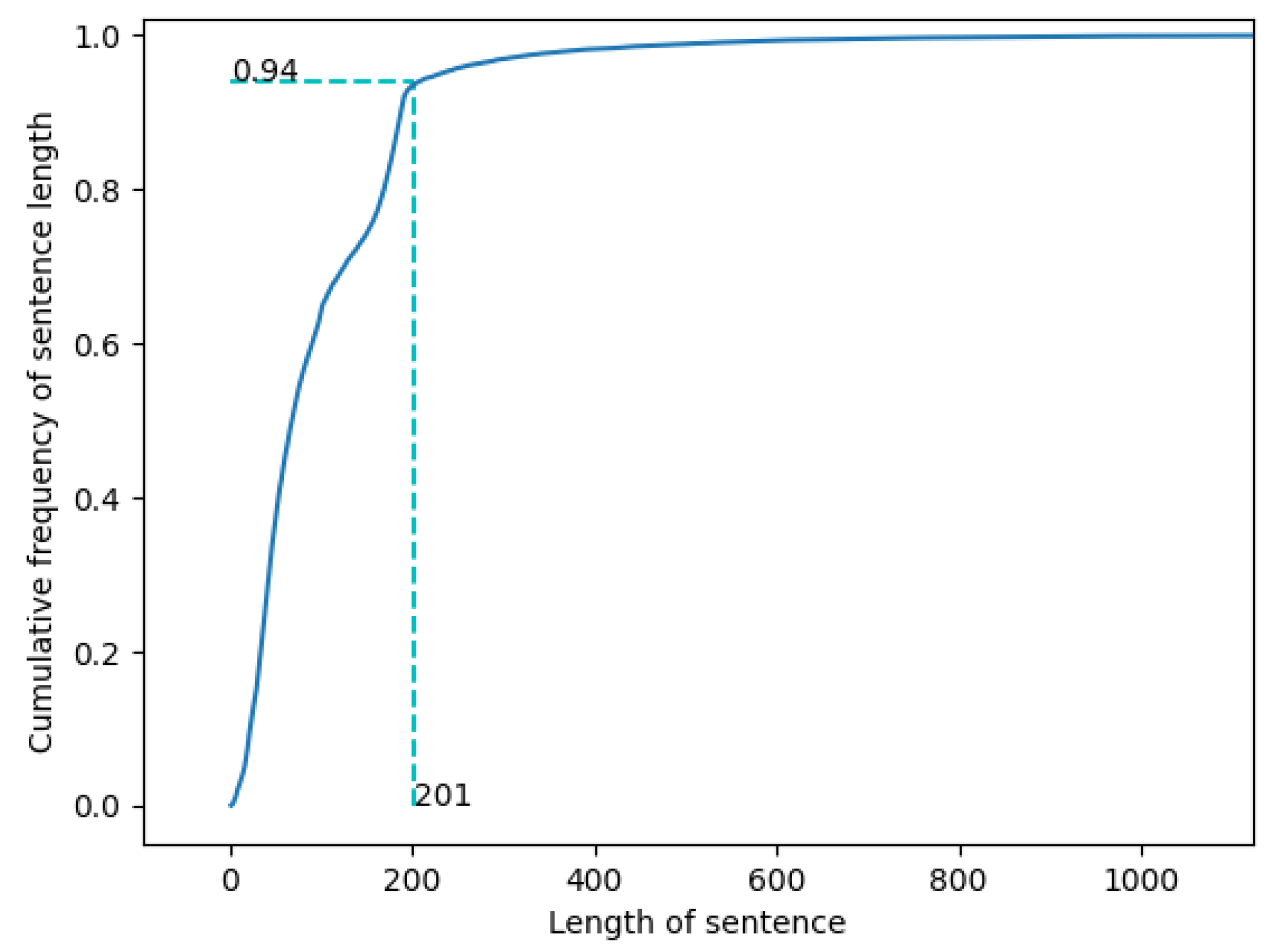
Figure 5 and Figure 6 demonstrate that the majority of the texts in the dataset have a length of less than 200 words, with only a small portion have more than 200. Sentences with a text length of less than 200 words appear most frequently. When the text length is 201, the cumulative frequency of sentences is 0.94. Consequently, this paper considers both the length of the text and its frequency of occurrence and selects 200 as the length of the input text.

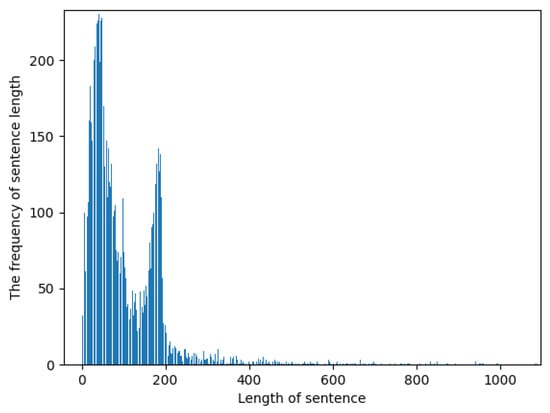
Figure 5. Sentence length and frequency statistics.

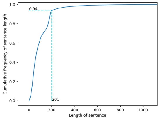
Figure 6. Graph of the cumulative distribution function of sentence length.

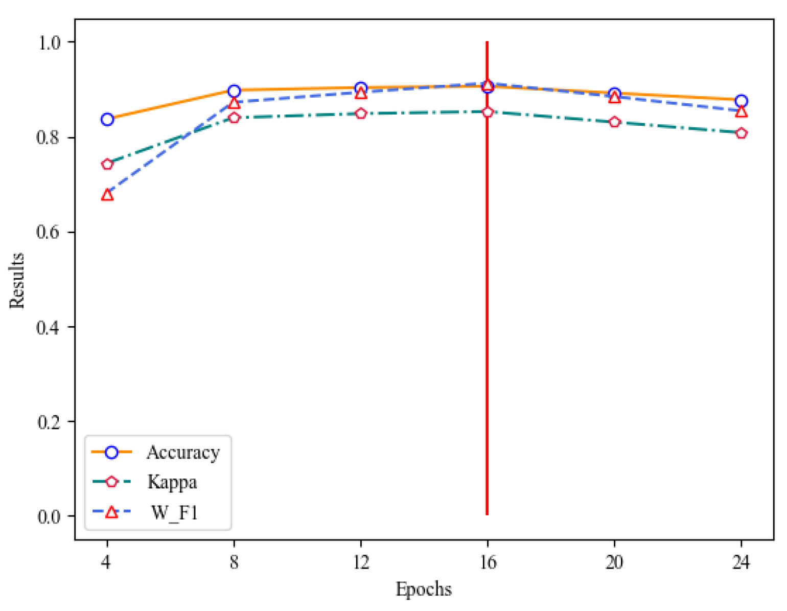
The selection of the number of iterations is a critical factor in determining the model’s quality. Too many iterations can lead to over-fitting, while too few can prevent the model from reaching its best state. As Figure 7 and Table 3 demonstrate, the model’s performance begins to decline when the number of iterations exceeds 16, and the performance of the model improves when it is less than 16. After analyzing the experimental data, it is concluded that 16 is the optimal number of iterations.

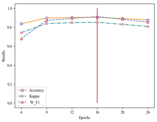
Figure 7. Selection of epochs.

Table 3. Selection of epochs.

Epochs	Accuracy	Kappa	W-F1 Score
4	0.8367	0.7431	0.6801
8	0.8978	0.8397	0.8722
12	0.9033	0.8483	0.8934
16	0.9061	0.8528	0.9126
20	0.8917	0.8304	0.8843
24	0.8774	0.8082	0.8542

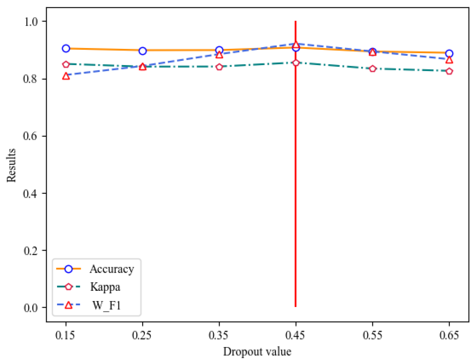
Model training is susceptible to over-fitting, as evidenced by a low loss function on the training data and a high prediction accuracy, yet a large loss function and low accuracy on the test data. To prevent this, we introduce a dropout value, which makes the model more generalizable by reducing the complex co-adaptive relationships between neurons. Experimentation has shown that the model performs best when the dropout value is 0.45, thus preventing over-fitting. The outcomes are depicted in Table 4 and Figure 8.

Table 4. Selection of dropout value.

Dropout	Accuracy	Kappa	W-F1 Score
0.15	0.9045	0.8507	0.8118
0.25	0.8985	0.8411	0.8431
0.35	0.8988	0.8414	0.8846
0.45	0.9078	0.8555	0.9213
0.55	0.8940	0.8342	0.8943
0.65	0.8895	0.8264	0.8671

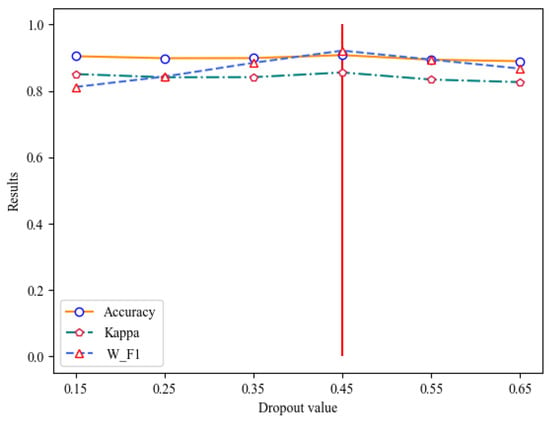
Figure 8. Selection of dropout value.

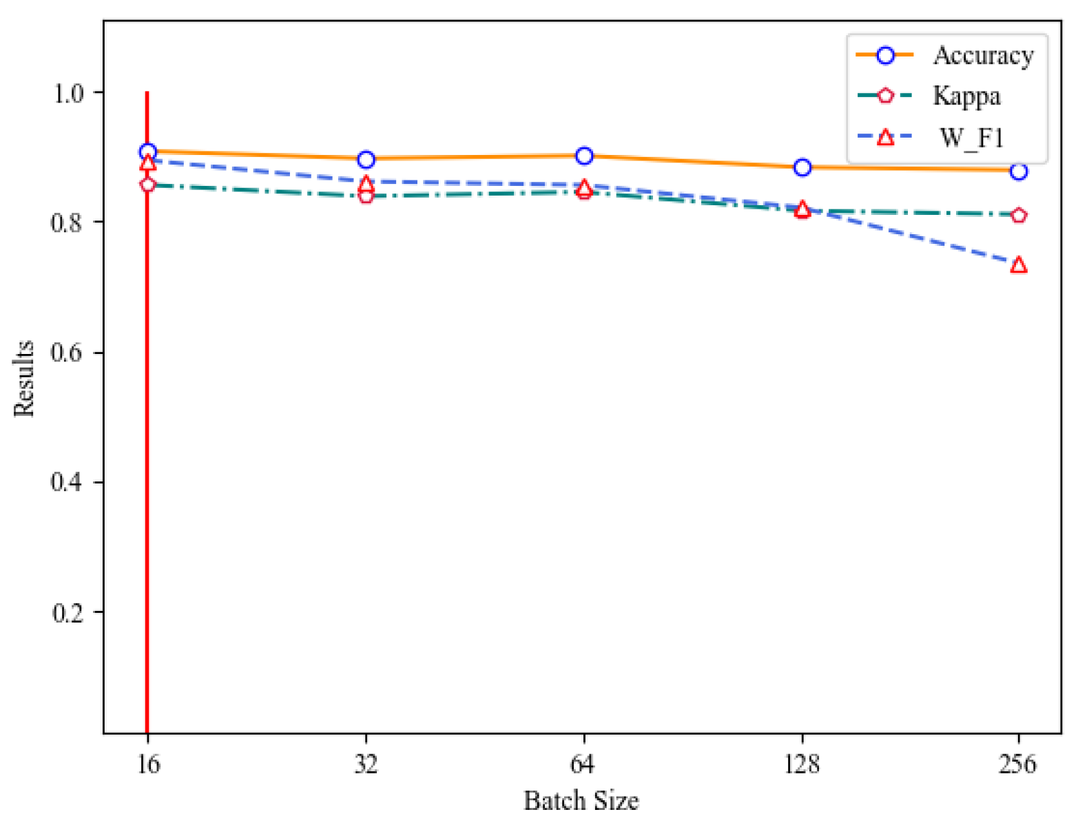
The batch size, which is the number of samples selected for one training, influences the optimization degree and speed of the model. By setting the batch size, the model can select batch data for processing each time during the training process. If batch size is too large [30], the network tends to converge to sharp minima, potentially resulting in poor generalization. To ensure the best training effect, an appropriate batch size should be chosen. Experimentally, when the batch size is set to 16, the convergence accuracy is maximized, as illustrated in Table 5 and Figure 9.

Table 5. Selection of batch size.

Batch Size	Accuracy	Kappa	W-F1 Score
16	0.9083	0.8563	0.8943
32	0.8971	0.8389	0.8617
64	0.9014	0.8455	0.8562
128	0.8836	0.8166	0.8215
256	0.8793	0.8111	0.7358

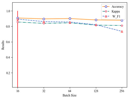
Figure 9. Selection of batch size.

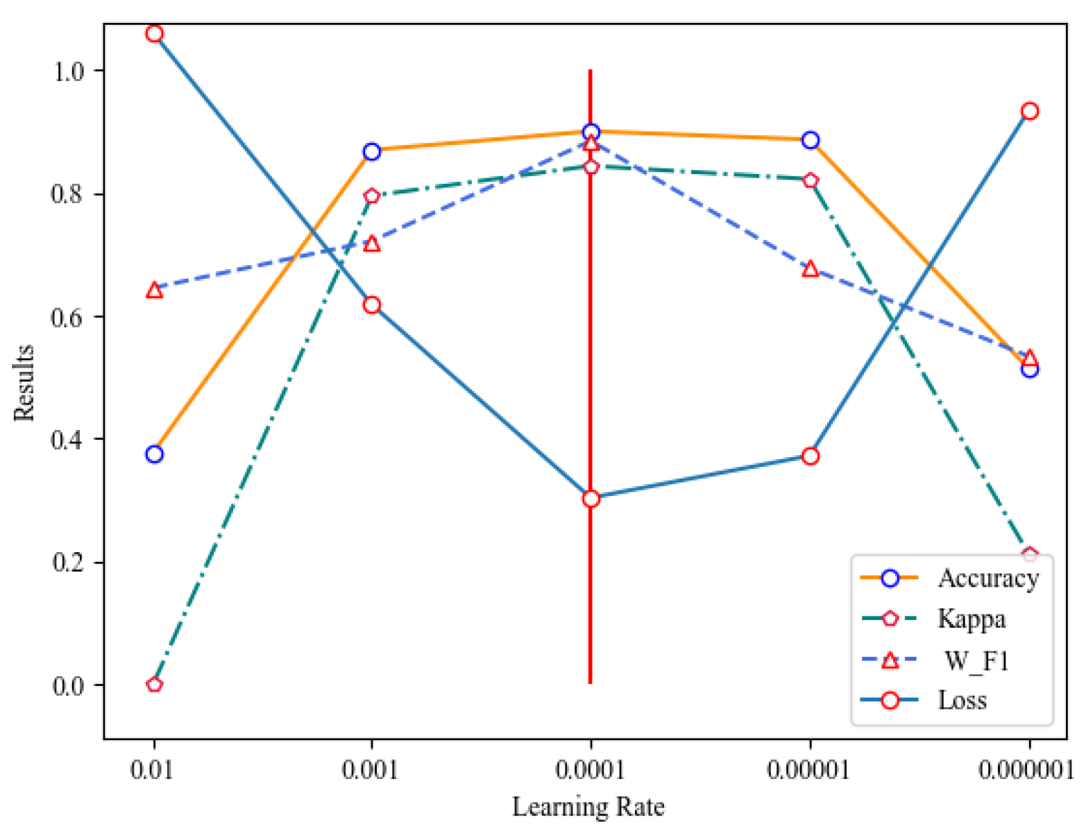
The learning rate determines whether the objective function can converge to the local minimum and when it can converge to the minimum. An appropriate learning rate can make the objective function converge to the local minimum within an appropriate time. If the learning rate is too large, the loss will explode, and if the learning rate is too small, the loss will not change for a long time. In this paper, we attempt to use different learning rates, observe the relationship between the learning rates and the loss, and find the learning rate corresponding to the quickest loss rate. The results, shown in Table 6 and Figure 10, indicate that the model performs best at a learning rate of 0.0001, at which the loss decreases the fastest.

Table 6. Selection of learning rate.

Learning Rate	Accuracy	Loss	Kappa	W-F1 Score
0.01	0.3770	1.0600	0.000	0.6452
0.001	0.8696	0.6178	0.7951	0.7213
0.0001	0.9002	0.3036	0.8438	0.8843
0.00001	0.8867	0.3721	0.8222	0.6774
0.000001	0.5142	0.9329	0.2133	0.5342

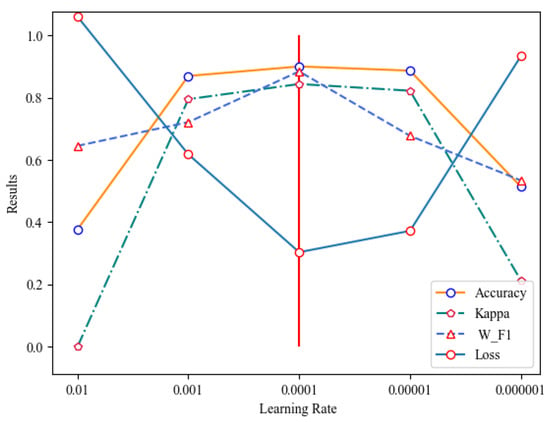
Figure 10. Selection of learning rate.

Comparison training was performed with other hyperparameter value combinations to ensure that the hyperparameter combination in this paper is optimal. Finally, the hyperparameters of the model in this paper, as well as those of the comparison model, are detailed in Table 7.

Table 7. The setting of model hyperparameters.

Hyperparameter	Hyperparameter Value
Latitude of word vector	128
Convolution kernel size	3
Number of convolution kernels	250
The BiLSTM hides layer size	64
Maximum input text length	200
Epoch number	16
Dropout value	0.45
Batch size	16
Learning rate	0.0001

5.5. Model Comparison

To assess the performance of the proposed model, we conducted comparative experiments using eight deep learning models with similar architectures [19,23,31,32,33,34,35,36].

Analysis of Table 8 reveals that the proposed model exhibits a superior accuracy rate, Kappa coefficient, and weighted F1 score. This is due to the incorporation of the attention mechanism and BiLSTM network into the CNN. The BiLSTM network facilitates the extraction of features from the input text sequence, taking into account both past and future information. This leads to a 1.07% improvement in accuracy and a 2.26% improvement in weighted F1 score compared to the CNN model alone. The attention mechanism further enhances the model’s performance by allowing it to focus on emotion-related words or sentences while discarding emotion-irrelevant text content. As a result, the proposed model outperforms other deep learning models.

Table 8. Deep learning models performance comparison.

Methods	Accuracy	Kappa	W-F1 Score
BiGRU [19]	0.9004	0.8441	0.8317
ATT+CNN [23]	0.9125	0.8629	0.8622
ATT+BiLSTM [31]	0.8976	0.8397	0.8803
CNN [32]	0.8966	0.8384	0.8546
LSTM+CNN [33]	0.8791	0.8103	0.8671
ATT+LSTM+CNN [34]	0.9016	0.8503	0.8869
CNN+BiLSTM [35]	0.9073	0.8555	0.8772
CNN+BiGRU [36]	0.8976	0.8402	0.8643
Proposed	0.9151	0.8673	0.8976

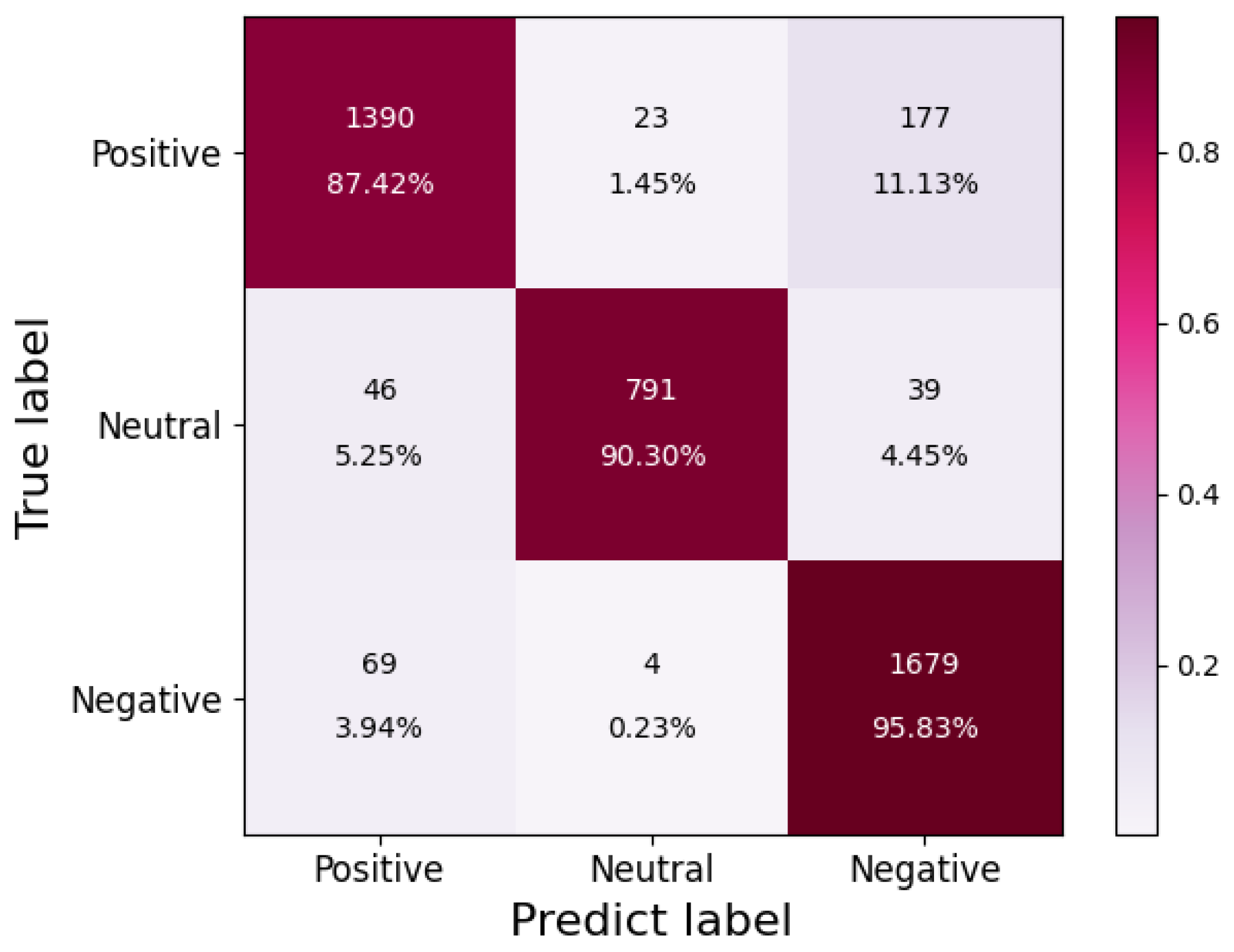
The confusion matrix in Figure 11 reveals the prediction accuracy of positive, neutral, and negative labels in the test set were 87.42%, 90.30%, and 95.83%, respectively. Notably, the accuracy of neutral and negative emotions exceeded 90%, indicating that this model is effective at multi-class sentiment analysis.

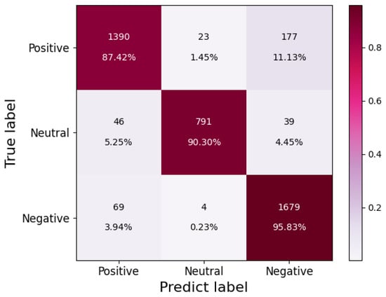
Figure 11. Test set confusion matrix.

As shown in Table 9, three mis-predicted examples are picked. Through the analysis, we found that the cause of the prediction errors was the classification problem of the labels and the tendency of some users to give a good rating even if they are not fully satisfied with the product. In addition, the semantic issues of the Chinese dataset make it more difficult to understand, which also brings certain difficulties to the correct recognition of the model.

Table 9. Examples of mispredictions.

Contents	True	Predict
It’s okay, but it’s too slow, the logistics took 4 days.	Positive	Negative
I don’t know if it’s good or not, I bought it for a friend, so I’ll give it five points.	Positive	Negative
Color, shape, okay, but the design is not so good.	Positive	Negative

5.6. Ablation Experiment

To assess the impact of the attention mechanism and BiLSTM on model performance, an ablation experiment was conducted.

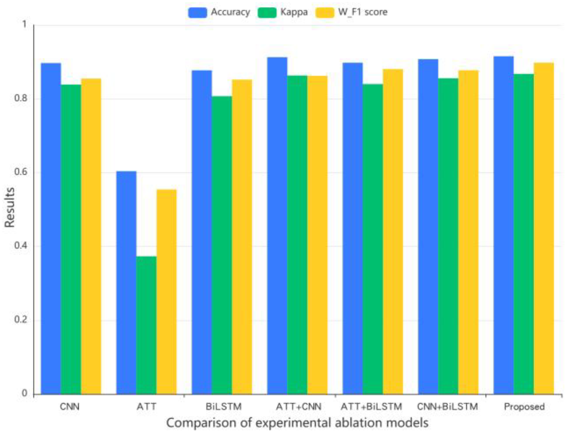
The results of the ablation experiment, shown in in Table 10 and Figure 12, reveal that the introduction of the attention mechanism alone into the sentiment analysis model yields poor performance, with an accuracy rate of 60.36%, a weighted F1 score of 0.5542, and a Kappa coefficient of 0.3731. Similarly, when only BiLSTM is used, the model can process text context information, resulting in an improved accuracy rate, Kappa coefficient, and weighted F1 score. It can be seen that the pure attention mechanism takes the shortest time, only 10.3 min. Although the training time is short, the performance of the model is the worst; it also takes less time to train BiLSTM and the CNN than the model proposed in this paper, but the accuracy rate, Kappa coefficient, and weighted F1 score are not as good as the model in this paper; the rest of the remaining models have better performances than the proposed model in terms of training time.

Table 10. Comparison of experimental ablation models.

Methods	Accuracy	Kappa	W-F1 Score	Time (mins)
CNN	0.8966	0.8384	0.8546	36.4
ATT	0.6036	0.3731	0.5542	10.3
BiLSTM	0.8770	0.8068	0.8518	39.2
ATT+CNN	0.9125	0.8629	0.8622	49.5
ATT+BiLSTM	0.8976	0.8397	0.8803	51.2
CNN+BiLSTM	0.9073	0.8555	0.8772	54.3
Proposed	0.9151	0.8673	0.8976	47.8

Figure 12. Comparison of experimental ablation models.

The combination of the attention mechanism and BiLSTM enables the model to not only consider text information from both directions but also to focus on emotion-related sentences, thus improving the model’s performance, and it does not take a lot of time. This paper’s model yields an accuracy 1.85% higher than that of the CNN alone, 31.15% higher than that of the ATT alone, and 0.78% higher than that of ATT+CNN, which significantly enhances the model’s feature extraction and classification capabilities, resulting in optimal performance.

6. Conclusions

Sentiment analysis is a significant branch of NLP, and its application for e-commerce platforms is highly valued by both consumers and businesses. This paper proposes a model architecture, AB-CNN, which combines an attention mechanism and BiLSTM to enhance the accuracy of multi-classification models. The attention mechanism extracts words or sentences related to emotion, while BiLSTM simultaneously captures contextual text information, further strengthening the emotion degree and improving the model’s classification prediction performance. Finally, the proposed model is benchmarked against existing literature on similar architectures, yielding the best experimental results.

The limitations of the current work include the following: (1) we only compared models with similar architectures (2) and hyperparameter settings that favored our proposed approach. In the future work, to improve the model, we could use the Bert or transformer pre-training model. Additionally, due to the complexity of Chinese text itself, we could try to introduce a powerful Chinese sentiment dictionary to improve the prediction accuracy.

References

- Hu, R.; Rui, L.; Zeng, P.; Chen, L.; Fan, X. Text sentiment analysis: A review. In Proceedings of the 2018 IEEE 4th International Conference on Computer and Communications (ICCC), Chengdu, China, 7–10 December 2018; pp. 2283–2288. [Google Scholar]
- Peng, H.; Cambria, E.; Hussain, A. A review of sentiment analysis research in Chinese language. Cogn. Comput. 2017, 9, 423–435. [Google Scholar] [CrossRef]
- Zargari, H.; Zahedi, M.; Rahimi, M. GINS: A Global intensifier-based N-Gram sentiment dictionary. J. Intell. Fuzzy. Syst. 2021, 40, 11763–11776. [Google Scholar] [CrossRef]
- Yan, X.; Huang, T. Research on construction of Tibetan emotion dictionary. In Proceedings of the 2015 18th International Conference on Network-Based Information Systems, Taipei, Taiwan, 2–4 September 2015; pp. 570–572. [Google Scholar]
- Wang, S.M.; Ku, L.W. ANTUSD: A large Chinese sentiment dictionary. In Proceedings of the Tenth International Conference on Language Resources and Evaluation (LREC’16), Portorož, Slovenia, 23–28 May 2016; pp. 2697–2702. [Google Scholar]
- Zhang, S.; Wei, Z.; Wang, Y.; Liao, T. Sentiment analysis of Chinese micro-blog text based on extended sentiment dictionary. Future. Gener. Comput. Syst. 2018, 81, 395–403. [Google Scholar] [CrossRef]
- Jia, K.; Li, Z. Chinese micro-blog sentiment classification based on emotion dictionary and semantic rules. In Proceedings of the 2020 International Conference on Computer Information and Big Data Applications (CIBDA), Guiyang, China, 17–19 April 2020; pp. 309–312. [Google Scholar]
- Xu, G.; Yu, Z.; Yao, H.; Li, F.; Meng, Y.; Wu, X. Chinese text sentiment analysis based on extended sentiment dictionary. IEEE Access 2019, 7, 43749–43762. [Google Scholar] [CrossRef]
- Tran, T.K.; Phan, T.T. A hybrid approach for building a Vietnamese sentiment dictionary. J. Intell. Fuzzy. 2018, 35, 967–978. [Google Scholar] [CrossRef]
- Wei, W.; Cao, X.; Li, H.; Shen, L.; Feng, Y.; Watters, P.A. Improving speech emotion recognition based on acoustic words emotion dictionary. Nat. Lang. Eng. 2021, 27, 747–761. [Google Scholar] [CrossRef]
- Miao, G.H. Emotion Mining and Simulation Analysis of Microblogging Based on Word2vec and SVM. J. Electron. Sci. Technol. 2018, 31, 81–83. [Google Scholar]
- Xue, J.; Liu, K.; Lu, Z.; Lu, H. Analysis of Chinese Comments on Douban Based on Naive Bayes. In Proceedings of the 2nd International Conference on Big Data Technologies, Jinan, China, 28–30 August 2019; pp. 121–124. [Google Scholar]
- Wawre, S.V.; Deshmukh, S.N. Sentiment classification using machine learning techniques. Int. J. Sci. Res. 2016, 5, 819–821. [Google Scholar]
- Kamal, A.; Abulaish, M. Statistical features identification for sentiment analysis using machine learning techniques. In Proceedings of the 2013 International Symposium on Computational and Business Intelligence, New Delhi, India, 24–26 August 2013; pp. 178–181. [Google Scholar]
- Rathor, A.S.; Agarwal, A.; Dimri, P. Comparative study of machine learning approaches for Amazon reviews. Procedia. Comput. Sci. 2018, 132, 1552–1561. [Google Scholar] [CrossRef]
- Zhang, Y.; Wang, L. Design of Employee Comment Sentiment Analysis Platform Based on AE-SVM Algorithm. J. Phys. Conf. Ser. 2020, 1575, 012019. [Google Scholar] [CrossRef]
- Mitroi, M.; Truică, C.O.; Apostol, E.S.; Florea, A.M. Sentiment analysis using topic-document embeddings. In Proceedings of the 2020 IEEE 16th International Conference on Intelligent Computer Communication and Processing (ICCP), Cluj-Napoca, Romania, 3–5 September 2020; pp. 75–82. [Google Scholar]
- Teng, F.; Zheng, C.; Li, W. Multidimensional topic model for oriented sentiment analysis based on long short-term memory. J. Comput. Appl. 2016, 36, 2252. [Google Scholar]
- Yin, X.; Liu, C.; Fang, X. Sentiment analysis based on BiGRU information enhancement. J. Phys. Conf. Ser. 2021, 1748, 032054. [Google Scholar] [CrossRef]
- He, J.; Zou, M.; Liu, P. Convolutional neural networks for chinese sentiment classification of social network. In Proceedings of the 2017 IEEE International Conference on Mechatronics and Automation (ICMA), Takamatsu, Japan, 6–9 August 2017; pp. 1877–1881. [Google Scholar]
- Zeng, J.; Ma, X.; Zhou, K. Enhancing attention-based LSTM with position context for aspect-level sentiment classification. IEEE Access 2019, 7, 20462–20471. [Google Scholar] [CrossRef]
- Zhou, J.; Lu, Y.; Dai, H.N.; Wang, H.; Xiao, H. Sentiment analysis of Chinese microblog based on stacked bidirectional LSTM. IEEE Access 2019, 7, 38856–38866. [Google Scholar] [CrossRef]
- Su, Y.J.; Chen, C.H.; Chen, T.Y.; Cheng, C.C. Chinese microblog sentiment analysis by adding emoticons to attention-based CNN. J. Internet. Technol. 2020, 21, 821–829. [Google Scholar]
- Truică, C.O.; Apostol, E.S.; Șerban, M.L.; Paschke, A. Topic-based document-level sentiment analysis using contextual cues. Mathematics 2021, 9, 2722. [Google Scholar] [CrossRef]
- Petrescu, A.; Truică, C.O.; Apostol, E.S.; Paschke, A. EDSA-Ensemble: An Event Detection Sentiment Analysis Ensemble Architecture. arXiv 2023, arXiv:2301.12805. [Google Scholar]
- Treisman, A. Features and objects in visual processing. Sci. Am. 1986, 255, 114B–125. [Google Scholar] [CrossRef]
- Hochreiter, S.; Schmidhuber, J. Long short-term memory. Neural. Comput. 1997, 9, 1735–1780. [Google Scholar] [CrossRef]
- Huang, P.; Zheng, L.; Wang, Y.; Zhu, H.J. Sentiment Analysis of Chinese Text Based on CNN-BiLSTM Serial Hybrid Model. In Proceedings of the 2021 10th International Conference on Computing and Pattern Recognition, Shanghai China, 15–17 October 2021; pp. 309–313. [Google Scholar]
- Xu, F.; Zhang, X.; Xin, Z.; Yang, A. Investigation on the Chinese text sentiment analysis based on convolutional neural networks in deep learning. Comput. Mater. Con. 2019, 58, 697–709. [Google Scholar] [CrossRef]
- Keskar, N.S.; Mudigere, D.; Nocedal, J.; Smelyanskiy, M.; Tang PT, P. On large-batch training for deep learning: Generalization gap and sharp minima. arXiv 2016, arXiv:1609.04836. [Google Scholar]
- Long, F.; Zhou, K.; Ou, W. Sentiment analysis of text based on bidirectional LSTM with multi-head attention. IEEE Access 2019, 7, 141960–141969. [Google Scholar] [CrossRef]
- Liao, S.; Wang, J.; Yu, R.; Sato, K.; Cheng, Z. CNN for situations understanding based on sentiment analysis of twitter data. Procedia. Comput. Sci. 2017, 111, 376–381. [Google Scholar] [CrossRef]
- Zhang, W.; Li, L.; Zhu, Y.; Yu, P.; Wen, J. CNN-LSTM neural network model for fine-grained negative emotion computing in emergencies. Alex. Eng. J. 2022, 61, 6755–6767. [Google Scholar] [CrossRef]
- Jiang, M.; Zhang, W.; Zhang, M.; Wu, J.; Wen, T. An LSTM-CNN attention approach for aspect-level sentiment classification. J. Comput. Methods Sci. Eng. 2019, 19, 859–868. [Google Scholar] [CrossRef]
- Gan, C.; Feng, Q.; Zhang, Z. Scalable multi-channel dilated CNN–BiLSTM model with attention mechanism for Chinese textual sentiment analysis. Future. Gener. Comput. Syst. 2021, 118, 297–309. [Google Scholar] [CrossRef]
- Miao, Y.; Ji, Y.; Peng, E. Application of CNN-BiGRU Model in Chinese short text sentiment analysis. In Proceedings of the 2019 2nd International Conference on Algorithms, Computing and Artificial Intelligence, Sanya China, 20–22 December 2019; pp. 510–514. [Google Scholar]
Disclaimer/Publisher’s Note: The statements, opinions and data contained in all publications are solely those of the individual author(s) and contributor(s) and not of MDPI and/or the editor(s). MDPI and/or the editor(s) disclaim responsibility for any injury to people or property resulting from any ideas, methods, instructions or products referred to in the content. |
© 2023 by the authors. Licensee MDPI, Basel, Switzerland. This article is an open access article distributed under the terms and conditions of the Creative Commons Attribution (CC BY) license (https://creativecommons.org/licenses/by/4.0/).