Abstract
In the study of non-intrusive load monitoring, using a single feature for identification can lead to insignificant differentiation of similar loads; however, multi-feature fusion can pool the advantages of different features to improve identification accuracy. Based on this, this paper proposes a recognition method based on feature fusion and matrix heat maps, using V-I traces, phase and amplitude of odd harmonics, and fundamental amplitude. These are converted into matrix heat maps, which can retain both large and small eigenvalues of the same feature for different loads and can retain different features. The matrix heat map is recognized by using SE-ResNet18, which avoids the problem of the classical CNN depth being too deep, causing network degradation and being difficult to train, and achieves trauma-free monitoring of home loads. Finally, the model is validated using the PLAID and REDD datasets, and the average recognition accuracy is 96.24% and 96.4%, respectively, with significant recognition effects for loads with similar V-I trajectories and multi-state loads.
1. Introduction
The two main approaches used in existing load monitoring systems can be categorized under non-intrusive load monitoring (NILM) and intrusive load monitoring (ILM). ILM involves installing smart power plugs directly at each electrical socket. NILM does not intrude upon the occupants during data collection and only requires the installation of a single power meter for the entire floor or building [1]. NILM does not disturb the occupants during the data collection process and only one meter has to be installed. Therefore, NILM is one of the important directions for future smart grid development. It can not only help users to adjust their own electricity consumption behavior and save electricity, but also help the grid to realize fine-grained load sensing, accurately profile user behavior, and offer differentiated and precise services [2]. For the moment, load-monitoring has been applied to power system diagnostics [3], smart energy management [4], appliance recognition [5], and energy dashboards [6].
Early NILM used single features for identification, and the common features include active power, reactive power, current waveform, steady-state current harmonics, power harmonics [7,8,9,10], and V-I trajectory [11], among which V-I trajectory has better identification [12]. However, with V-I trajectory it is difficult to distinguish loads with similar trajectories. Power features are difficult to distinguish with low-power loads and harmonic currents cannot distinguish loads with less current distortion. Therefore, multi-feature fusion has become a current research hotspot. Yi Sun et al. proved that harmonic features can effectively distinguish low-power loads and fuse the third harmonic with power [13]. Z Zheng et al. verified that harmonic current features are additive, and a multilayer perceptron classifier is constructed using harmonic current features to accurately identify typical nonlinear and resistive loads [14]. Shouxiang Wang et al. used convolutional neural networks and BP neural networks to convert V-I trajectories and power into vectors before fusion, but the overall training time of the model is long, and it is prone to the problem of local minima [15].
Some scholars transformed the signal data into image data and used image recognition techniques for recognition. De Baets L et al. encoded the signal data into images and used V-I trajectories to generate binary images, but some features of V-I trajectories disappeared after conversion to binary images [16]. Junfeng Chen et al. constructed load identification by Gram matrix color coding [17]. Xiang Y et al. first converted the power and current magnitude of the load into color information by color coding, and then fused the features with the V-I trajectory. However, the fused image had a single color, the power and current differed greatly between loads and determining the color by power or amplitude will lead to most of the loads having lower power or current concentrated in the same color interval, which will affect the recognition accuracy [18]. Finally, this literature used convolutional neural networks (CNN) for recognition, and as the number of layers of the network increased, the model degenerated and the gradient exploded or disappeared [19].
Based on this, a non-intrusive load monitoring method based on multi-feature fusion and image recognition is proposed in this paper. The voltage and current of the V-I trajectory, the amplitude and phase of the odd harmonics, and the fundamental amplitude are converted into numerical values. Then, a feature matrix is built, in which the features are superimposed according to the number of times they appear at each position, and then the superimposed matrix is color-coded according to the size of the values and converted into a matrix heat map. Finally, a residual network18 (ResNet18) with squeeze and excitation (SE) is used for image recognition. This paper effectively solves the similarity load identification problem and the masking problem of features generated when performing feature fusion. Unlike most related solutions [20,21], the proposed NILM approach does not use a dedicated one-to-one model for each load but is implemented on the basis of a single multi-class classifier. That is, one model is used to identify multiple loads, i.e., one model is used to identify several loads. Therefore, it is more computationally efficient [22]. The average recognition accuracy of the proposed method is 96.24% and 96.4% for loads with similar V-I trajectories, 96% and 94.9% for loads with similar V-I trajectories, and 97.79% and 96.5% for different states of the same load, respectively, when tested with PLAID and REDD datasets, and compared with other recognition methods. The results show that the proposed method has higher accuracy.
2. Feature Construction
2.1. Single-Class Feature Processing
V-I traces are extracted by event detection. Detecting the load start-stop event, the voltage before the load is turned on is , and the voltage after it is turned on is . Accordingly, the current before it is turned on is , and the current after it is turned on is . Before and after the cut the voltage does not change much and, considering the possibility of certain fluctuations, the average voltage before and after the event is calculated as follows:
Using a differential extraction method that uses the current after the event minus the current before the event, it is possible to obtain the load data for the start-up:
The V-I trajectory can be formed by taking the voltage and current in one cycle as the horizontal and vertical coordinates, respectively [11].
Figure 1 shows the V-I trajectories of several loads with large differences, and Figure 2 shows the V-I trajectories with large similarities, in which the voltage and current data have been normalized.
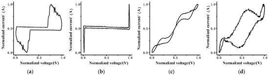
Figure 1.
Typical load V-I trajectory diagram for (a) compact fluorescent lamp, (b) laptop, (c) fridge, (d) washing machine.
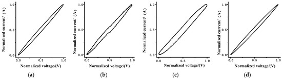
Figure 2.
V-I trajectory diagram of similar load for (a) coffee maker, (b) hair dryer, (c) incandescent light bulb, (d) kettle.
Decomposition of the steady-state current signal using the fast Fourier transform (FFT) is as follows:
where , , is the amplitude of each harmonic, and , , is the phase angle of each harmonic.
The load of Figure 2 was harmonic decomposed, and it was compared and found that the fundamental of the load has a large variability with the 3rd, 5th, 7th, and 9th harmonics, see Figure 3. Fusing it with the V-I traces can improve the resolution.
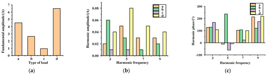
Figure 3.
(a) Base wave amplitude, (b) odd harmonic amplitudes, (c) odd harmonic phase.
Harmonic amplitude and phase are numerically large and fusing them with V-I traces requires data processing for voltage, current, and amplitude phase. To normalize the selected data:
where: denotes the original value and denotes the minimum value of a period. denotes the maximum value of a period. denotes the normalized value.
Rounding of the normalized data is as follows:
where: and denote the finalized eigenvalue. denotes fundamental amplitude. denotes quotient. denotes remainder. denotes rounding down. denotes the order of the matrix.
2.2. Matrix Heat Map Construction
Create a 32 × 32 matrix and draw grid lines. Determine the position of the features in the matrix in the form of values in (,(31-)), (,), (,), (,). Write the corresponding values at (m, n) of the matrix according to the number of occurrences of the features to form the feature matrix, where: i denotes the number of harmonics (i = 3, 5, 7, 9) and (m, n) denotes the position of the mth row and nth column in the matrix.
The feature matrix is converted to RGB images according to the size of the values, and according to the definition of the matrix heat map, the larger the value, the darker the color. The opposite is lighter. A sample set consisting of matrix heat maps with multiple features is constructed. The matrix heat map has a significant improvement in feature resolution for similar loadings after adding color features. Taking the coffee machine and the kettle in the similarity load of Figure 2 as an example, binarizing the matrix heat map shows that the feature locations in the matrix are largely similar and not very distinguishable. However, as shown in the Figure 4, when comparing this with the matrix heat map, the feature differentiation between the two loads increases after adding the color features.
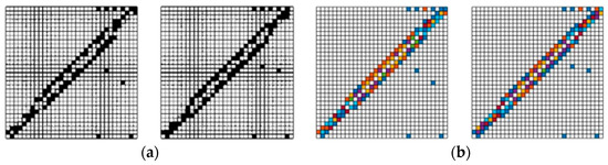
Figure 4.
(a) Binary diagram of coffee machine and kettle. (b) Matrix heat map of coffee machine and kettle.
3. Identification Network Construction
CNN is widely used in the field of image classification. The edges and contours of the images are extracted by convolutional computation, which reduces the complexity of the model by reducing a large number of parameters into a small number of parameters. When the image is rotated, inverted, or deformed, the image can be recognized [19]. However, the problem of model degradation and gradient explosion or disappearance occurs as the depth of the network increases. Based on this, SE-ResNet adds a residual network with squeeze and excitation (SE) to the CNN to improve the accuracy of the model effectively by showing the interdependence between modeling channels and adaptively calibrating the features of the channel directions accordingly.
3.1. ResNet Network Structure
ResNet adds shortcut connection branches outside the convolutional layer to perform a simple constant mapping and to form the basic residual learning units, and then solves the problem of network degradation that is difficult to train when the CNN network is too deep by sequentially stacking the residual learning units, making it possible to train deep convolutional neural networks.
Figure 5 shows the standard network structure and the ResNet structure. The basic residual learning unit neither introduces new parameters nor increases the computational complexity.
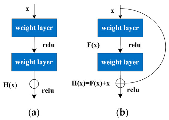
Figure 5.
(a) Standard network structure diagram. (b) ResNet structure diagram.
The principle of ResNet is:
where: is the direct mapping and is the activation function.
The residual block can be expressed as:
The relationship between the deeper L layer and the l layer is:
According to the chain rule for derivatives used in backward propagation, the gradient of the loss function with respect to is
Throughout the training process, cannot be −1 all the time, so there is no problem of gradient disappearance in the residual network, and means that the gradient of L layer can be directly passed to any l layer that is shallower than it.
After converting numerical features to image features, the number of samples in the dataset decreases and does not require too much network depth, so ResNet18 is used in this paper, and the structure diagram is shown in Figure 6.
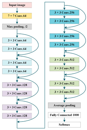
Figure 6.
ResNet18 structure diagram.
The features extracted by CNN through convolutional layer stacking are high-dimensional features. Some of them are lost, while the residual block of ResNet is to skip the extraction of features by some convolutional layers and fuse the features before n layers, with the convolutional features after n layers, so that both high-dimensional features and low-dimensional features are retained, and the network performance is improved. Global average pooling is also used to replace the fully connected layer (fc) in the classical CNN. The global average pooling strengthens the correspondence between feature maps and categories on the fully connected layer, which is more suitable for convolutional structures. In addition, there are no parameters to be optimized in the global average pooling, which avoids overfitting. Furthermore, global average pooling aggregates spatial information and is more robust with regard to spatial transformation of the input.
3.2. SE-ResNet
SE-ResNet focuses on the interdependencies between the convolved feature channels using 1D convolution. The SE block is completed by a squeeze operation, which summarizes the overall information of each feature mapping, and an excitation operation, which scales the importance of each feature mapping. In this way, the squeeze operation extracts only the significant information of each channel, and the excitation operation computes the dependencies between channels using a fully connected layer with a nonlinear function.
The difference between the SE-ResNet and ResNet network structures is shown in Figure 7.
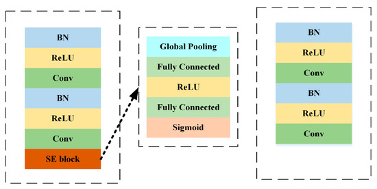
Figure 7.
Network structure of SE-ResNet and ResNet.
3.3. Identification Process
The recognition process in this paper is shown in Figure 8, which contains data acquisition, data preprocessing, feature construction, and training and recognition using SE-ResNet.
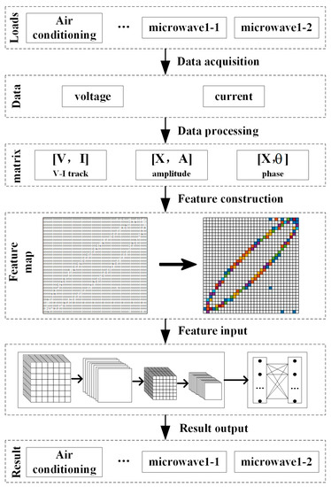
Figure 8.
Identification flow chart.
In the identification process, firstly, the data acquisition equipment collects voltage and the current data of each type of load from the home, normalizes the voltage and current data, and also extracts harmonic features from the current waveform by FFT, including the amplitude and phase. The three types of feature data are processed and written into a matrix to form a feature matrix, which is converted into a matrix heat map. The matrix heat map of each type of load is made into a sample set and divided into a training set and a test set, which is put into SE-ResNet for training and testing.
4. Experimental Results of REDD and PLAID
In the actual arithmetic example, the deep learning framework of tensorflow 2.0 is used to construct a sample set consisting of a matrix heat map from the PLAID dataset as well as the REDD dataset in the way described in this paper. After the sample set is produced, 80% of each class is selected as the training set and 20% as the test set. The confusion matrix is used to evaluate the recognition accuracy of the method proposed in the article. Each column of the confusion matrix represents the predicted category, and the total number of each column represents the number of data predicted to be in that category. Each row represents the true attribution category of the data, and the total number of each row represents the number of data instances in that category. The value of each column represents the number of real data predicted as that category. From the confusion matrix, TP, FP, FN, and TN can be calculated, where TP means that the predicted result is true and the actual result is also true, FP means that the predicted result is true and the actual result is false, FN means that the predicted result is false and the actual result is true, and TN means that the predicted result is false and the actual result is also false. The precision rate (P), recall rate (R), summed average of precision and recall (F1), and accuracy rate (A) can be calculated from TP, FP, FN, and TN. P and R can measure the correctness of a positive sample, and the higher the index result, the better. The formulas for calculating each indicator are as follows:
4.1. REDD
The nine loads in the REDD dataset are represented using the numbers shown in Table 1 below: 1-1, 1-2 denote different states of the same device and electric light 2 and electric light 3 denote two different light loads.

Table 1.
Symbols representing the load of the REDD dataset.
The load identification results for the REDD dataset are shown in Figure 9 and Figure 10: green represents the number and percentage of correctly identified samples and yellow represents the number and percentage of incorrectly identified samples.
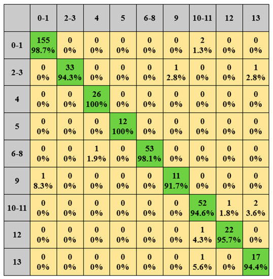
Figure 9.
REDD dataset identification results. (Green means true, yellow means false).
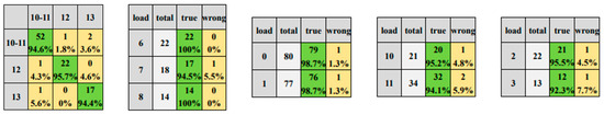
Figure 10.
Identification results of multi-state load and similar load. (Green means true, yellow means false).
From the results, it can be seen that the correct identification rate of each type of load is above 91.7%, among which the light 1 and light 2 reach 100%, with an average correct rate of 96.4%. Similarly, for the load socket, washer dryer, and electric furnace, the correct identification rate is more than 94.4%, and the average correct rate is 94.9%. The correct recognition rate of multi-state devices such as the fridge, light, microwave, and socket is above 92.3%, and the average correct rate reaches 96.5%.
Table 2 is evaluated by P, R, F1, and A. As can be seen from Table 2, most of the P, R, F1, and A of various types of loads were kept at 0.85 and above, and light 3 reached 1, with the average values of 0.95, 0.96, 0.96, and 0.99, respectively.
Table 2.
Evaluation indexes of confusion matrix.
4.2. PLAID
The 15 loads in PLAID were identified. The load representation is shown in Table 3, and the multi-state loads are represented in the same way as in the previous example.
Table 3.
Symbols representing the load of the PLAID dataset.
The results of load identification are shown in Figure 11 and Figure 12. The correct identification rate of each type of load is above 90.8%, and the correct identification rate of the hair curler, laptop and vacuum is 100%, and the average correct rate is 96.24%. Among these, although the kettle is still affected by the similarity load resulting in a slightly lower recognition correct rate than the other loads, the overall correct recognition rate reaches 92%, which is higher than the correct rate generated using the original V-I trajectory.
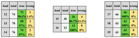
Figure 11.
Identification results of multi-state load. (Green means true, yellow means false).
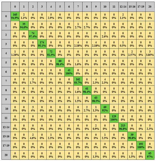
Figure 12.
PLAID dataset identification results. (Green means true, yellow means false).
Meanwhile, the correct recognition rate of the soldering iron is affected by the number of samples and lower than the other loads. However, in terms of the number of incorrectly identified samples, the recognition of the soldering iron is not worse than that of other loads. The multi-state loads such as the microwave, soldering iron, and vacuum have a correct recognition rate of 86.7% or more for each state, with a 100% correct recognition rate for each type of state for vacuum, and an average correct rate of 97.79% for each type of state for multi-state loads. The results of the identification of the four similar loads described previously are shown in Figure 11. As can be seen from Figure 11, the average correct identification rate is 96%. Table 4 evaluates by P, R, F1, and A. Most of the index values are kept at 0.82 and above, among which the hair curler, laptop, and vacuum reach 1.00, and the average values are 0.96, 0.96, 0.96, and 0.99, respectively.
Table 4.
Evaluation indexes of confusion matrix.
4.3. Comparative Analysis of Results
Using the same dataset, sample sets made of different features are selected and compared using different recognition models to evaluate the effectiveness of different methods in terms of recognition correctness or F1 values.
As shown in Table 5, the literature that identifies the REDD dataset quantifies the V-I trajectory and uses the SoftMax classifier for identification with an F1 value of 0.88 and quantifies only a single feature V-I trajectory. The similarity load will be difficult to identify with similar quantified values. CNN or SE-ResNet networks are used to identify the V-I trajectory binary map, the binary map after fusion of V-I trajectory and harmonics, and matrix heat map. The feature class, fusion method, and identification network are changed to form a control group, and the average F1 value of the proposed method in this paper is 0.99, which is a better result compared with other control groups.
Table 5.
Comparison of results of different methods based on REDD data sets.
As shown in Table 6, in the literature on identifying PLAID datasets, Gao J et al. [12] and De Baets Leen et al. [16] used random forests for the identification of V-I302 trajectories; however, with a single feature, random forests have a long training time and high data requirements, otherwise they are prone to overfitting. Shouxiang Wang et al. proposed a feature fusion of V-I trajectories with power, using different networks for feature extraction and, after feature input to the network, the output vectors of the hidden layers of the two neural networks were combined together to form a composite vector feature, which was recognized using BP neural networks with a correct rate of 83.7% [15]. Xiang Y et al. uses power and current magnitudes incorporated into V-I trajectories to form true color feature images for recognition by CNN, but the true color image of each type of load is a single color, while the color is determined by the power and current magnitudes, which can lead to the difficulty in distinguishing the true color image because the power or current values of individual loads are too large, making most of the loads concentrated in the same color interval, such as microwave ovens and washing machines. In this paper, the data intervals are evenly distributed in a 32 × 32 matrix, making the loads in the same range of value intervals show more significant color variability [18]. Z Zheng et al. used amplitude and phase angle composition features and a multilayer perceptron for recognition [14]. De Baets L et al. used CNN for recognition with a correct rate of 77.60% [23]. Meanwhile, for matrix heat map recognition using CNN and SE-ResNet network respectively, the correct rate was 89.35% and 96.24%, which proves that the SE-ResNet network is better than CNN under the same conditions.
Table 6.
Comparison of results of different methods based on PLAID data sets.
After the above comparison, it was found that the studies of Wang Shouxiang et al. [15] and Xiang Y et al. [18] were based on the same dataset, PLAID, and the overall recognition results were better, but some of the loads were not recognized with high accuracy, such as: air condition, fan, fridge, heater, and washing machine. As shown in Figure 13, the accuracy of this paper’s method for identifying such loads is higher than the above literature. For the PLAID dataset, the current study generally selects 11 load types to be carried out, and this paper also identifies four other types of other loads: blender, coffee maker, hair curler, and soldering iron, and the identification accuracy is higher than 91%.
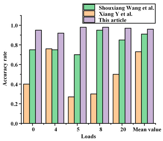
Figure 13.
Load comparison diagram of low identification accuracy.
Instead of using a dedicated one-to-one model for each device, the method proposed in the article is implemented on the basis of a single multiclass classifier, where one model is used for multiple devices with higher computational efficiency. SE-ResNet adds residual connectivity and an SE block completed by squeeze and excitation operations to the CNN, and although it still needs to be retrained when new devices are added, the overall training time of the model is greatly reduced. The proposed method is trained on the REDD dataset with six houses and the PLAID dataset with 56 houses, which indicates that the method is scalable and generalizable, and the addition of more house data is to be continued to be tested on new datasets. Follow-up work should investigate how the proposed method in this paper can reduce the training volume and improve the computational efficiency when identifying new devices.
5. Conclusions
In this paper, a non-intrusive load monitoring method based on multi-feature fusion with image recognition technology is proposed. When performing feature fusion, the V-I trajectory, amplitude and phase angle of odd harmonics, and fundamental wave amplitude are fused into a feature matrix. The matrix heat map is constructed by color according to the magnitude of the values, which effectively solves the feature masking problem arising from feature fusion. In addition, the single feature similar load is well distinguished from the multi-state load. In terms of image recognition, the SE-ResNet network recognition model is built to avoid the gradient descent problem of CNN, and also to realize the use of one classifier model to recognize multiple loads, which shortens the training time and improves the computational efficiency. Two datasets, the PLAID dataset and the REDD dataset, were used for validation, and the results prove that the proposed method has better accuracy compared with other methods.
In the existing research, the features used in the methods with high recognition rates are mostly transient features, which have low computational efficiency and high data collection and storage costs. In this paper, a one-to-many algorithm model is used for recognition, which improves the computational efficiency to some extent, but adding new loadings requires retraining. In future research, the balance degree between accuracy and computational efficiency should be considered. For example, migration learning might be used to reduce the training time. Furthermore, the correlation could be fused between loads with steady-state features to improve the accuracy of recognition, using steady-state features.
Author Contributions
Method, T.C. and H.Q.; analysis and verification, H.Q. and W.W.; writing, H.Q.; review, T.C., X.L. and W.Y. All authors have read and agreed to the published version of the manuscript.
Funding
This research was supported by the National Natural Science Foundation of China (51907104), The Opening Fund of Hubei Province Key Laboratory of Operation, and Control of Cascade Hydropower Station (2019KJX08).
Data Availability Statement
All the data supporting the reported results have been included in this paper.
Conflicts of Interest
The authors declare no conflict of interest.
References
- Tekler, Z.D.; Low, R.; Zhou, Y.; Yuen, C.; Blessing, L.; Spanos, C. Near-real-time plug load identification using low-frequency power data in office spaces: Experiments and applications. Appl. Energy 2020, 275, 115391. [Google Scholar] [CrossRef]
- Deng, X.P.; Zhang, G.Q.; Wei, Q.L.; Wei, P.; Li, C.D. A survey on the non-intrusive load monitoring. Acta Autom. Sin. 2022, 48, 644–663. [Google Scholar]
- Shaw, S.R.; Leeb, S.B.; Norford, L.K.; Cox, R.W. Nonintrusive load monitoring and diagnostics in power systems. IEEE Trans. Instrum. Meas. 2008, 57, 1445–1454. [Google Scholar] [CrossRef]
- Tekler, Z.D.; Low, R.; Yuen, C.; Blessing, L. Plug-Mate: An IoT-based occupancy-driven plug load management system in smart buildings. Build. Environ. 2022, 223, 109472. [Google Scholar] [CrossRef]
- Ridi, A.; Gisler, C.; Hennebert, J. A survey on intrusive load monitoring for appliance recognition. In Proceedings of the 2014 22nd International Conference on Pattern Recognition, Stockholm, Sweden, 24–28 August 2014; IEEE: Piscataway, NJ, USA, 2014; pp. 3702–3707. [Google Scholar]
- Tekler, Z.D.; Low, R.; Blessing, L. User perceptions on the adoption of smart energy management systems in the workplace: Design and policy implications. Energy Res. Soc. Sci. 2022, 88, 102505. [Google Scholar] [CrossRef]
- Bonfigli, R.; Principi, E.; Fagiani, M.; Severini, M.; Squartini, S.; Piazza, F. Non-intrusive load monitoring by using active and reactive power in additive Factorial Hidden Markov Models. Appl. Energy 2017, 208, 1590–1607. [Google Scholar] [CrossRef]
- Liang, J.; Ng, S.K.; Kendall, G.; Cheng, J.W. Load signature study-Part I: Basic concept, structure, and methodology. IEEE Trans. Power Deliv. 2009, 25, 551–560. [Google Scholar] [CrossRef]
- He, D.; Du, L.; Yang, Y.; Harley, R.; Habetler, T. Front-end electronic circuit topology analysis for model-driven classification and monitoring of appliance loads in smart buildings. IEEE Trans. Smart Grid 2012, 3, 2286–2293. [Google Scholar] [CrossRef]
- Wichakool, W.; Avestruz, A.T.; Cox, R.W.; Leeb, S.B. Modeling and estimating current harmonics of variable electronic loads. IEEE Trans. Power Electron. 2009, 24, 2803–2811. [Google Scholar] [CrossRef]
- Mulinari, B.M.; de Campos, D.P.; da Costa, C.H.; Ancelmo, H.C.; Lazzaretti, A.E.; Oroski, E.; Lima, C.R.; Renaux, D.P.; Pottker, F.; Linhares, R.R. A new set of steady-state and transient features for power signature analysis based on VI trajectory. In Proceedings of the 2019 IEEE PES Innovative Smart Grid Technologies Conference-Latin America (ISGT Latin America), Gramado, Brazil, 15–18 September 2019; IEEE: Piscataway, NJ, USA, 2019; pp. 1–6. [Google Scholar]
- Gao, J.; Kara, E.C.; Giri, S.; Bergés, M. A feasibility study of automated plug-load identification from high-frequency measurements. In Proceedings of the 2015 IEEE Global Conference on Signal and Information Processing (GlobalSIP), Orlando, FL, USA, 13–16 December 2015; IEEE: Piscataway, NJ, USA, 2015; pp. 220–224. [Google Scholar]
- Yi, S.; Can, C.; Jun, L.; Jianhong, H.; Xiangjun, L. A Non-Intrusive Household Load Monitoring Method Based on Genetic Optimization. First Power Syst. Technol. 2016, 40, 3912–3917. [Google Scholar] [CrossRef]
- Zheng, Z.; Chen, H.; Luo, X. A supervised event-based non-intrusive load monitoring for non-linear appliances. Sustainability 2018, 10, 1001. [Google Scholar] [CrossRef]
- Wang, S.X.; Guo, L.Y.; Chen, H.W.; Deng, X.Y. Non-intrusive Load Identification Algorithm Based on Feature Fusion and Deep Learning. Autom. Electr. Power Syst. 2020, 44, 103–110. [Google Scholar]
- De Baets, L.; Develder, C.; Dhaene, T.; Deschrijver, D. Automated classification of appliances using elliptical fourier descriptors. In Proceedings of the 2017 IEEE International Conference on Smart Grid Communications (SmartGridComm), Dresden, Germany, 23–27 October 2017; IEEE: Piscataway, NJ, USA, 2017; pp. 153–158. [Google Scholar]
- Chen, J.; Wang, X.; Zhang, H. Non-intrusive load recognition using color encoding in edge computing. Chin. J. Sci. Instrum. 2020, 41, 12–19. [Google Scholar] [CrossRef]
- Xiang, Y.; Ding, Y.; Luo, Q.; Wang, P.; Li, Q.; Liu, H.; Fang, K.; Cheng, H. Non-Invasive Load Identification Algorithm Based on Color Coding and Feature Fusion of Power and Current. Front. Energy Res. 2022, 10, 534. [Google Scholar] [CrossRef]
- Gai, R.L.; Cai, J.R.; Wang, S.Y. Research Review on Image Recognition Based on Deep Learning. J. Chin. Comput. Syst. 2021, 42, 1980–1984. [Google Scholar]
- Ji, T.Y.; Liu, L.; Wang, T.S.; Lin, W.B.; Li, M.S.; Wu, Q.H. Non-Intrusive Load Monitoring Using Additive Factorial Approximate Maximum a Posteriori Based on Iterative Fuzzy c-Means. IEEE Trans. Smart Grid 2019, 10, 6667–6677. [Google Scholar] [CrossRef]
- Culler, D. BuildSys’15: The 2nd ACM International Conference on Embedded Systems for Energy-Efficient Built Environments, Seoul, Republic of Korea, 4–5 November 2015; Association for Computing Machinery: New York, NY, USA, 2015. [Google Scholar]
- Athanasiadis, C.L.; Papadopoulos, T.A.; Doukas, D.I. Real-time non-intrusive load monitoring: A light-weight and scalable approach. Energy Build. 2021, 253, 111523. [Google Scholar] [CrossRef]
- De Baets, L.; Ruyssinck, J.; Develder, C.; Dhaene, T.; Deschrijver, D. Appliance classification using VI trajectories and convolutional neural networks. Energy Build. 2018, 58, 32–36. [Google Scholar] [CrossRef]


Disclaimer/Publisher’s Note: The statements, opinions and data contained in all publications are solely those of the individual author(s) and contributor(s) and not of MDPI and/or the editor(s). MDPI and/or the editor(s) disclaim responsibility for any injury to people or property resulting from any ideas, methods, instructions or products referred to in the content. |
© 2023 by the authors. Licensee MDPI, Basel, Switzerland. This article is an open access article distributed under the terms and conditions of the Creative Commons Attribution (CC BY) license (https://creativecommons.org/licenses/by/4.0/).