Abstract
An iterative design algorithm is developed for robust disturbance–rejection control of uncertain systems with time-varying parameter perturbations in this paper. For more design degrees of freedom, a generalized equivalent-input-disturbance estimator is adopted to approximate the effect of both disturbances and uncertainties. By the bound real lemma, the norm is used to evaluate the robust disturbance–rejection performance of the closed-loop uncertain system. To avoid the constraints introduced by the widely used commutative condition, the control gains are divided into two groups and calculated by steps. Further, two robust quadratic stability conditions are derived, and an iterative design algorithm is developed to optimize the robust disturbance–rejection performance. Finally, the effectiveness and advantages of the developed method are demonstrated by a case study of a suspension system of modern vehicles.
1. Introduction
Practical systems often suffer from unknown disturbances and uncertainties. They deteriorate control accuracy and even destabilize the systems [1]. For these reasons, disturbance–rejection control is one of the key issues in control practice.
To improve the disturbance–rejection performance, many strategies have been developed [2,3]. They can be mainly divided into two categories [4]. The passive methods use a common feedback loop to handle multiple control objectives at the same time, which include robust stability, disturbance rejection, noise suppression, etc. By considering the unknown disturbances and uncertainties as an overall disturbance, the active methods introduce an additional loop, specifically for disturbance estimation and suppression control, resulting in better control performance [5,6].
By utilizing all the information of system states, the uncertainty and disturbance estimator is developed by assuming any signals can be properly approximated by filtering [7,8]. The disturbance observer in the frequency domain is composed of a filter and an inverse dynamic of a nominal plant [9]. It may be a bit tricky to design the filter to simultaneously fulfill causality, robust stability, and disturbance–rejection performance. Some techniques were performed to ease the design [10]. The disturbance observer in the time domain is built on known disturbance models [11,12]. The extended-state observer is applicable to more general systems, which is another effective method for integral systems with matched disturbances or mismatched disturbances that can be transformed into matched ones [13]. The generalized extended-state observer is applicable to general systems. However, a static or dynamic compensation gain is usually required for mismatched disturbance [14,15].
Focusing on the influence of disturbances or uncertainties on the system output, the equivalent-input-disturbance (EID) approach is developed for simple and effective disturbance–rejection control [16]. An EID is a virtual disturbance defined on the control input, which has the same effect on the system output as the real disturbances do. Since the EID approach provides an estimate of the disturbances or uncertainties on the control input, it does not require the disturbance compensation gain. That is to say, it is usually useful for both matched and mismatched disturbances [17,18]. Moreover, only output information is required for EID estimation. It uses only output information and does not need the direct availability of system states, the disturbance model, the differentiation of measured outputs, or an inverse dynamics of a plant. So, it is easy to implement.
In engineering practice, it is difficult to obtain a precise mathematical model of a physical system, owning to parameter perturbations, modeling errors, unmodeled dynamics, and other factors. Moreover, as explained by [19], the uncertainties impact the disturbance–rejection control performance. So, it is vital and necessary to design a robust controller with a prescribed disturbance–rejection performance index. A robust controller was designed for an uncertain system [20], but some constraints were introduced by using the commutative condition. By taking the uncertainties into account, a parameter design method was developed for an improved EID-based system in [21], but it cannot guarantee disturbance–rejection performance. A disturbance–rejection control method with performance was developed in [22], but it was designed in the frequency domain. Some expertise may be needed to select the weighting functions.
In this paper, an iterative design algorithm is developed for an uncertain system with unknown disturbances. The EID approach is applied to handle the disturbances. The Luenberger observer is constructed to reproduce the system states. Then, a feedback controller is designed to stabilize the closed-loop uncertain system. Finally, an optimization design algorithm is given. The major contributions of this paper are given as below.
- A generalized EID estimator (GEID) with a general filter is developed, which enables handling disturbances in a specified frequency range.
- For the sake of less conservatism, the control gains are divided into two groups and designed in steps.
- Two robust quadratic stability conditions are derived in terms of linear matrix inequalities (LMIs), which guarantee the prescribed performance of the closed-loop uncertain system.
- An iterative design algorithm is presented to optimize the performance of the closed-loop uncertain control system.
The remainder of this paper is organized as below. The system configuration is explained in Section 2. Section 3 analyzes the dynamics of the GEID-based disturbance–rejection control system. Section 4 presents conditions with prescribed disturbance–rejection performance. A design procedure is presented in Section 5. The validity and superiority of the developed method are demonstrated by Section 6. Section 7 concludes this paper. Further, a consolidated list of variables and acronyms in this paper is given by two tables in Appendix A.
In this paper, denotes the set of real matrices; denotes an identity matrix of size n; I and 0 stand for identity and zero matrices with compatible dimensions, respectively; and denote the transpose and inverse of a matrix P, respectively; denotes the Laplace transform of a time signal ; the time t and the complex frequency s are omitted when the content is clear; denotes the transfer matrix from to ; denotes the norm of the transfer matrix ; denotes ; and a symmetric matrix is denoted by .
2. Configuration of GEID-Based Disturbance–Rejection Control System
Consider an uncertain plant subject to an exogenous disturbance.
where , , are the state, input, and output of the plant, respectively; is an unknown disturbance; A, B, , C, and D are dimensioned real constant matrices; and and are time-varying uncertainties in the following general structure
where M, , and are known real constant matrices; and is a time-varying real function matrix with Luenberger measurable elements while satisfying
Note the uncertainties considered in the control system appear only in the state matrix A and the output matrix C.
The time-varying parameter perturbations of the system matrix and output matrix are considered in this paper. Many scenarios fall into this case [23].
Assumption 1.
Assumption: The system (1) is controllable and observable.
Assumption 2.
Assumption: The disturbance is bounded, i.e.,
where is the 2-norm of and is an unknown upper bound.
Assumption 1 is standard for system design [24], and Assumption 2 usually holds in practice.
As illustrated in Figure 1, the control structure of the developed GEID-based robust control system includes a plant, a state observer, a GEID estimator, and a state-feedback controller based on observed states.
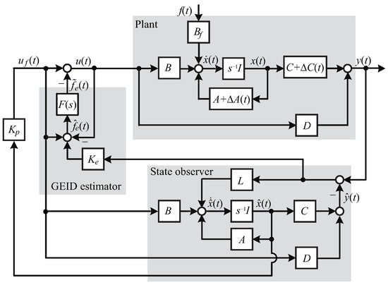
Figure 1.
Robust disturbance–rejection control system with generalized equivalent-input-disturbance (GEID) estimator.
Since is unknown, lump them as .
When the full-state is not available or too costly, a state observer with full order is constructed to produce the states of the plant (1). Some design strategies of the state observer were talked about in [25,26]. In this paper, the observer system is viewed as the ideal dynamic of the real plant (1)
where , are the state, input, and output of the observer, respectively; and L is the observer gain to be determined.
The EID approach is adopted for active disturbance rejection control. As analyzed in [16], the filter is of great importance to the performance. For disturbances in a low-frequency range, a first-order low-pass filter satisfying the following condition is good enough.
where the angular frequency is the bandwidth of the low-pass filter and determined by the disturbance–rejection control design. However, when there exist tight constrains on control bandwidth [19] or specific performance requirements on the middle-frequency range, a general filter is necessary. Superior to the conventional EID one, the GEID approach is able to estimate disturbances of a more general frequency range by a general filter.
In this paper, a GEID estimator is adopted for EID estimation, where a control gain is introduced to adjust the control performance and a general filter is used for a general design task. A state–space representation of is
where is the state of the filter; and are the unfiltered and filtered estimates of the EID, respectively. For simplicity, denote
Further, an equivalent description of the GEID estimator is
When is selected to have full column rank, we have with being the Moore-Penrose generalized inverse of . In the sequel, calculating is performed by designing .
Based on the observed state , the original state-feedback control law is
where is the feedback control gain to be determined. It is used to stabilize the controlled system.
By introducing a degree of freedom in the inner loop for disturbance estimation and compensation, the new control law is
3. Dynamics of GEID-Based Control System
Define
and
Define
From (11) to (17), we have the following state–space description for the closed-loop uncertain control system in Figure 1:
where
It is clear that the separation theorem cannot be used due to the parameter uncertainties, and the control gains to be determined scatter in the system matrix. To be specific, the feedback control gain is located on the right-hand side of some elements, while the control gains L and of the observer and GEID estimator are related to the right-hand side.
Inspired by [27], to reduce the conservatism of parameter design by removing the constraints from the widely used commutative condition, the control gains , L, and of the feedback controller, the state observer, and the GEID estimator are divided into two groups, and (L, ). Additionally, they are designed by steps.
First, when is assigned prior to L and , the state–space model (18) and (19) is used for system design. For this purpose, rewrite
where
On the other hand, let
The closed-loop uncertain control system can also be represented by
where
Further, for the closed-loop uncertain control system in Figure 1, the transfer matrix from to y can be written by or , where
4. Design of GEID-Based Control System
To facilitate the presentation, we recall the following lemmas.
Lemma 1
(Bounded real lemma [28]). Given , the following two statements are equivalent:
- 1.
- The system matrix A is stable and .
- 2.
- There exists a symmetric, positive–definite matrix P, such that the following inequality holds.
Lemma 2
([29]). For given dimensioned matrices , H, F, and any satisfying
the following inequality holds
if and only if there is an positive constant ε, such that
Lemma 3
(Schur complement argument [30]). For any real symmetric matrix ∑,
we have the following equivalent assertion:
- 1.
- ;
- 2.
- and ;
- 3.
- and .
With known , a robust stability condition together with the gains of (L, ), are given as below, which guarantees the disturbance–rejection performance of the closed-loop uncertain control system, i.e.,
Theorem 1.
For a prescribed positive scalar γ, select (, ), and give control gain if there exist a symmetric, positive–definite matrix P, a dimensioned matrix , and positive constants and , such that the following inequalities hold,
Then the GEID-based closed-loop uncertain control system in Figure 1 is robust stabilized and satisfies the robust performance condition (32). The blocks are given by
Further, the gains of the state observer and GEID estimator are, respectively,
where is the Moore-Penrose generalized inverse of .
Proof of Theorem 1.
Choose a candidate of the Lyapunov functional
where P is a symmetric, positive–definite matrix, which is defined in (35).
The derivative of along the GEID-based closed-loop uncertain control system (18) is
If
Then the system (18) is robust stabilized. Application of Lemma 2 to (39) shows that the GEID-based uncertain closed-loop control system is robust stable if the following matrix inequality holds.
where is a positive scalar. By Lemma 3, (40) is equivalent to the following inequality.
Substitution of (35) and (36) into (33) gives (41). Therefore, the closed-loop system is stabilized.
On the other hand, with known (L, ), the following theorem gives a design method for and guarantees the prescribed disturbance–rejection performance index (32).
Theorem 2.
For prescribed positive scalar γ, selected (, ), and given control gains (L, ), if there exist a symmetric, positive–define matrix , a dimensioned matrix , and positive constants and , such that the following inequalities hold,
where
then the GEID-based closed-loop uncertain control system in Figure 1 is stable and satisfies the robust performance condition (42). Further, the gain of the feedback controller is given by
Proof of Theorem 2.
A candidate of Lyapunov functional is selected as
where is a positive–definite, symmetric matrix defined in (44).
The derivative of along the GEID-based closed-loop uncertain control system (22) is
If
then the GEID-based closed-loop uncertain control system (22) is robust stable. By Lemma 2, if and only if there exists a positive constant , such that
then (48) holds. Pre- and post-multiplying the term on the left-hand side of (49) by gives
According to Lemma 3, (50) is equivalent to the following inequality.
Substituting (44) into (42) yields (51). Therefore, the closed-loop system is robust stabilized.
Remark 1.
Both Theorems 1 and 2 are robust stability conditions for the GEID-based closed-loop uncertain control system shown in Figure 1, which ensure the prescribed disturbance–rejection performance (32). When the gain of the feedback controller is known, Theorem 1 is applied to calculate the gains () of the observer and GEID; when () are known, Theorem 2 is adopted to compute .
Remark 2.
As for how to obtain a possible gain for Theorem 1 or a set of gains () for Theorem 2, as explained in [27], the gains which make the system matrix in (18) and in (22) Hurwitz, respectively, are appropriate. Note
where , , and are defined in (21). Therefore, a proper can be obtained by making in (18) Hurwitz, and an appropriate set of () can be gained to such that is Hurwitz.
5. Design Algorithm
Summarizing the aforementioned results gives the following iterative design procedure for the GEID-based uncertain control system, which optimizes the robust disturbance–rejection performance by minimize the performance index in (32). Further, the flowchart is shown in Figure 2.
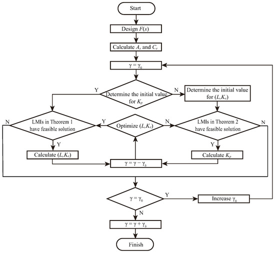
Figure 2.
Flowchart of the algorithm.
- Step 1:
- Choose an appropriate general filter , with being full column rank for the GEID estimator (8).
- Step 2:
- Calculate and according to (9).
- Step 3:
- Select an initial performance index and let .
- Step 4:
- Determine an initial value for the control gains or (L, ). If the initial value is determined for , go to Step 5; otherwise, go to Step 6.
- Step 5:
- Step 6:
- Step 7:
- Let , where is the decrease step. Determine the parameters to be optimized. If the known is used to optimize the gains (L, ), go to Step 5; otherwise, go to Step 6.
- Step 8:
- Adopt {, (L, )} and of the previous step as the finial gains and performance index, and end the design.
Remark 3.
In Step 1, the selection of is based on the frequency range of disturbance–rejection control. In Step 4, many methods can be used to obtain the initial values of and (L, ), such as the pole placement and linear quadratic regulator (LQR). In Step 7, it may take some trial and error to determine the iteration step and the iteration optimization sequence of control gains. For example, when (L, ) are too large, it is inappropriate to use them to optimize . The computation time of the developed design algorithm is usually dependent on the iterative search process. The computation time with a small iteration step is usually greater than that with a large one. In other words, there is a trade-off between the computation complexity and robust disturbance–rejection performance.
6. Case Study
In this section, a suspension system of modern vehicles is used to validate the developed method, which is responsible for ride safety and comfor. By the ISO2361, in the vertical direction, the human body is sensitive to vibrations within . So, the developed method is used to deal with the road disturbances over this range.
6.1. System Design
The parameters of the suspension system of a quarter-car model are
where , denotes the suspension deflection, is the tire deflection, is the speed of the car chassis, denotes the speed of the wheel assembly, y is the body vertical acceleration, and u is the active control input. The uncertainties are from a 1% time-varying perturbation in the stiffness of the suspension system. The parameter values of the suspension system are shown in Table 1.

Table 1.
Values of quarter-car model parameters.
Consider there is an isolated bump on an originally smooth road surface and the bump disturbance is given by
where , , and represent the amplitude, angular frequency, and period of the vibration, respectively. Assume , (i.e., 6 ), which belongs to the frequency range .
To mitigate the vibrations within , a Butterworth band-pass filter with this band-pass frequency range is chosen. The corresponding parameters are
According to (9), we have
Set the initial value of the performance index as
Use the LQR method to determine an initial value for the control gains (L, ) of the observer and GEID estimator. The weighting matrices are selected as
which give
For the performance index (56) and the above control gains (58), an application of Theorem 2 gives
Further, set the decrease step as
For in (59), by trail and error, we find there are no feasible solutions of (, ) to LMIs (33), and (34) of Theorem 1 due to the uncertainty blocks. Hence, the initial value (, ) is still used to optimize the control gain .
Thirteen iterations of Theorem 2 give
and
Then, we use the obtained gain in (62) to further optimize (L, ) by Theorem 1. For and , an application of Theorem 1 gives
Since there are no feasible solutions no matter for Theorem 1 or Theorem 2, we complete this design and use the following gains as the final control gains.
The robust disturbance–rejection performance of the closed-loop uncertain control system satisfies
The response of the GEID-based suspension control system is shown in Figure 3. As we can see, the closed-loop system is robust stabilized in the presence of the time-varying parameter perturbation and disturbance. The influences of parameter perturbation and disturbance on the system output, i.e., the body acceleration, have been well suppressed by the EID estimate of the GEID estimator.
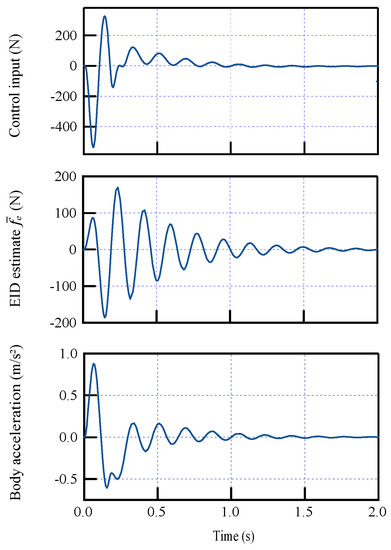
Figure 3.
System response of the developed GEID-based control method.
6.2. Comparisons with Other Methods
In this section, the developed method is compared with the passive control and the state-feedback control [31] for the nominal plant of the suspension system with and . The road disturbance is the same as (53).
First, the developed iterative design algorithm is applied. The band-pass filter is selected as the same as (54), which gives and in (55). Set the initial value of the performance index as
The initial control gains are chosen as the same as (58). Set the decrease step as
For the initial performance index (66), the control gains (58) and the decrease step (67) follow the developed iterative design algorithm by an alternate application of Theorems 1 and 2 until one of the two theorems has no feasible solutions. Finally, the performance index is decreased to
and the corresponding control gains and (L, ) are given as follows.
For the comparison with the full-state feedback control [31], the optimal performance index is , which is much greater than of the developed method. Further, the corresponding gain of the state feedback control is
The passive control method is also compared with the developed method. A passive suspension system is actually an open-loop control system without any controller.
The magnitude-frequency characteristics of the transfer matrices from the disturbance to the output of the GEID-based, full-state feedback, and passive control are illustrated in Figure 4. The developed GEID-based control system includes an observer, a state-feedback controller, and a GEID estimator. In the sate-feedback control system, a full-state feedback controller is devised by minimizing the disturbance–rejection performance index. However, it requires that all the states are available.
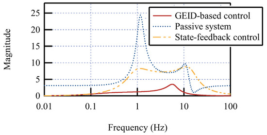
Figure 4.
Magnitude-frequency characteristics of disturbance–rejection transfer function.
The output responses of the proceeding three methods are shown in Figure 5. The corresponding optimal norm and the peak value of three control methods are given by Table 2.
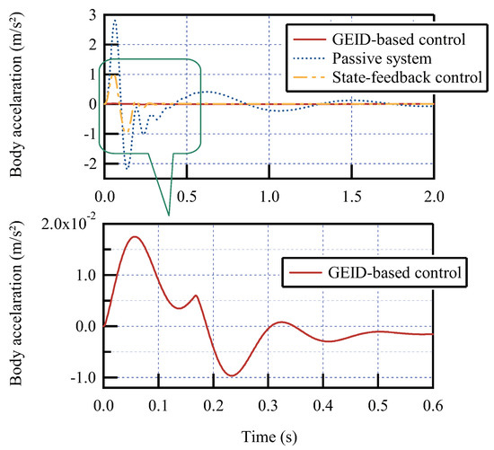
Figure 5.
Output response of body acceleration.
Table 2.
The optimal norm and the peak value of three control methods.
As we can see, although the full-state feedback control is much better than the passive control, the developed GEID-based disturbance–rejection method has much better disturbance–rejection performance than the full-state feedback control. Moreover, the maximum vertical acceleration of the body is only about 0.018 .
All in all, the developed iterative design method provides the best disturbance–rejection performance over the frequency band .
On the other hand, the full-state feedback control requires all states of the active suspension system, which may be costly and even difficult to achieve. All in all, the developed GEID-based control method has significant advantages over the state-feedback control method.
7. Conclusions
This paper presented an iterative design algorithm for the robust disturbance–rejection control of uncertain systems, which removed the constraints due to the widely used commutative condition. First, two state-space models were built for the closed-loop uncertain control system. By the bounded real lemma, the robust disturbance–rejection performance index was derived for performance optimization. Further, a robust stability condition was obtained. An iterative design algorithm was given, which guaranteed both robust stability and disturbance-rejection performance, Moreover, the gains of the state-feedback controller, the state observer, and the GEID estimator can be easily obtained by using the LMI-based technique. Finally, by a case study of a suspension control system of modern vehicles and comparisons with other methods, the effectiveness and advantages of the developed GEID-based iterative design method were clarified.
Author Contributions
Conceptualization, P.Y.; methodology, P.Y. and J.L.; software, J.L. and N.L.; validation, J.L., N.L. and H.Z.; formal analysis, J.L. and C.L.; investigation, N.L., H.Z. and C.L.; resources, J.L., N.L. and H.Z.; data curation, J.L.; writing—original draft preparation, P.Y. and J.L.; writing—review and editing, J.L. and N.L.; visualization, J.L. and N.L.; supervision, P.Y.; project administration, P.Y.; funding acquisition, P.Y. and C.L. All authors have read and agreed to the published version of the manuscript.
Funding
This work was supported by the National Natural Science Foundation of China under Grants 62003010 and 62273012, the Beijing Natural Science Foundation under Grant 4212933, and the Scientific Research Project of Beijing Educational Committee under Grant KM202110005023.
Data Availability Statement
The data are contained within the article.
Conflicts of Interest
The authors declare no conflict of interest.
Appendix A
This appendix contains a table of variable and acronym definitions used in the paper.
Table A1.
Acronyms.
Table A1.
Acronyms.
| Acronyms | Definition |
|---|---|
| EID | Equivalent-input-disturbance |
| GEID | Generalized equivalent-input-disturbance |
| LMIs | Linear matrix inequalities |
| LQR | Linear quadratic regulator |
Table A2.
Known parameters or variables.
Table A2.
Known parameters or variables.
| Known Parameters or Variables | Definition |
|---|---|
| A | System matrix |
| B | Input matrix |
| C | Output matrix |
| D | Direct transmission matrix |
| , and M | known real constant matrices of parameter uncertainties |
| Disturbance input channel | |
| General filter | |
| Feedback control gain | |
| L | Observer gain |
| GEID control gain |
References
- Liu, K.Z.; Yao, Y. Robust Control: Theory and Applications; Wiley: Hoboken, NJ, USA, 2016. [Google Scholar]
- Yang, J.; Cui, H.; Li, S.; Zolotas, A. Optimized active disturbance rejection control for DC-DC buck converters with uncertainties using a reduced-order GPI observer. IEEE Trans. Circuits Syst. Regul. Pap. 2018, 65, 832–841. [Google Scholar] [CrossRef]
- Xu, B.; Zhang, L.; Ji, W. Improved non-singular fast terminal sliding mode control with disturbance observer for PMSM drives. IEEE Trans. Transp. Electrif. 2021, 7, 2753–2762. [Google Scholar] [CrossRef]
- Chen, W.; Yang, J.; Guo, L.; Li, S. Disturbance observer-based control and related methods-an overview. IEEE Trans. Ind. Electron. 2016, 63, 1083–1095. [Google Scholar] [CrossRef]
- Miyamoto, K.; She, J.H.; Nakano, S.; Sato, D.; Chen, Y.L. Active structural control of base-Isolated building using equivalent-input-disturbance approach with reduced-order state observer. J. Dyn. Syst. Meas. Control. 2022, 144, 1081–1095. [Google Scholar] [CrossRef]
- Zhou, Y.; She, J.H.; Wang, F.; Iwasaki, M. Disturbance rejection for stewart platform based on integration of equivalent-input-disturbance and sliding-mode control methods. IEEE/ASME Trans. Mechatron. 2023, 1–11. [Google Scholar] [CrossRef]
- Stobart, R.K.; Kuperman, A.; Zhong, Q.C. Uncertainty and disturbance estimator-based control for uncertain LTI-SISO systems with state delays. J. Dyn. Syst. Meas. Control. 2011, 133, 024502. [Google Scholar] [CrossRef]
- Wu, Y.; Mahmud, M.H.; Zhao, Y.; Mantooth, H.A. Uncertainty and disturbance estimator-based robust tracking control for dual-active-bridge converters. IEEE Trans. Transp. Electrif. 2020, 6, 1791–1800. [Google Scholar] [CrossRef]
- Choi, Y.; Yang, K.; Chung, W.K.; Kim, H.R.; Suh, I.H. On the robustness and performance of disturbance observers for second-order systems. IEEE Trans. Autom. Control. 2003, 48, 315–320. [Google Scholar] [CrossRef]
- Li, M.; Yan, T.; Mao, C.; Wen, L.; Zhang, X.; Huang, T. Performance-enhanced iterative learning control using a model-free disturbance observer. IET Control. Theory Appl. 2021, 15, 978–988. [Google Scholar] [CrossRef]
- Xie, Y.; Qiao, J.; Yu, X.; Guo, L. Dual-disturbance observers-based control for a class of singularly perturbed systems. IEEE Trans. Syst. Man Cybern. Syst. 2022, 52, 2423–2434. [Google Scholar] [CrossRef]
- Cui, Y.; Qiao, J.; Zhu, Y.; Yu, X.; Guo, L. Velocity-tracking control based on refined disturbance observer for gimbal servo system with multiple disturbances. IEEE Trans. Ind. Electron. 2022, 69, 10311–10321. [Google Scholar] [CrossRef]
- Wang, L.X.; Zhao, D.X.; Zhang, Z.X.; Liu, Q.; Liu, F.C.; Jia, T. Model-free linear active disturbance rejection output feedback control for electro-hydraulic proportional system with unknown dead-zone. IET Control. Theory Appl. 2021, 15, 2081–2094. [Google Scholar] [CrossRef]
- Li, S.; Yang, J.; Chen, W.; Chen, X. Generalized extended state observer based control for systems with mismatched uncertainties. IEEE Trans. Ind. Electron. 2012, 59, 4792–4802. [Google Scholar] [CrossRef]
- Castillo, A.; Garcia, P.; Sanz, R.; Albertos, P. Enhanced extended state observer-based control for systems with mismatched uncertainties and disturbances. ISA Trans. 2018, 73, 1–10. [Google Scholar] [CrossRef]
- She, J.H.; Fang, M.; Ohyama, Q.; Hashimoto, H.; Wu, M. Improving disturbance-rejection performance based on an equivalent-input-disturbance approach. IEEE Trans. Ind. Electron. 2008, 55, 380–389. [Google Scholar] [CrossRef]
- Du, Y.; Cao, W.; She, J.H.; Wu, M.; Fang, M.; Kawata, S. Disturbance rejection and predictive control for systems with input and output delays. IEEE Trans. Syst. Man Cybern. Syst. 2022, 52, 4589–4599. [Google Scholar] [CrossRef]
- Huang, G.; She, J.H.; Fukushima, E.F.; Zhang, C.; He, J. Robust reconstruction of current sensor faults for PMSM drives in the presence of disturbances. IEEE/ASME Trans. Mechatronics 2019, 24, 919–2930. [Google Scholar] [CrossRef]
- Yu, P.; Liu, K.Z.; Wu, M.; She, J.H. Analysis of equivalent-input-disturbance-based control systems and a coordinated design algorithm for uncertain systems. Int. J. Robust Nonlinear Control. 2021, 31, 1755–1773. [Google Scholar] [CrossRef]
- Liu, R.J.; Liu, G.; Wu, M.; Xiao, F.; She, J.H. Robust disturbance rejection based on equivalent-input-disturbance approach. IET Control. Theory Appl. 2013, 7, 1261–1268. [Google Scholar] [CrossRef]
- Du, Y.W.; Cao, W.H.; She, J.H.; Wu, M.; Fang, M.X.; Seiichi, K. Disturbance rejection and robustness of improved equivalent-input-disturbance-based system. IEEE Trans. Cybern. 2022, 52, 8537–8546. [Google Scholar] [CrossRef]
- Yu, P.; Liu, K.Z.; Wu, M.; She, J.H. Improved equivalent-input-disturbance approach based on H∞ control. IEEE Trans. Ind. Electron. 2020, 67, 8670–8679. [Google Scholar] [CrossRef]
- Yu, P.; Liu, K.Z.; Li, X.L.; Yokoyama, M. Robust control of pantograph-catenary system: Comparison of 1-DOF-based and 2-DOF-based control systems. IET Control. Theory Appl. 2021, 15, 2258–2270. [Google Scholar] [CrossRef]
- Levine, W.S. The Control Handbook; CRC Press: Boca Raton, FL, USA, 1996. [Google Scholar]
- Sands, T.; Bollino, K.; Kaminer, I.; Healey, A. Autonomous minimum safe distance maintenance from submersed obstacles in ocean currents. J. Mar. Sci. Eng. 2018, 6, 98. [Google Scholar] [CrossRef]
- Sands, T. Virtual sensoring of motion using pontryagin’s treatment of hamiltonian systems. Sensors 2021, 21, 4603. [Google Scholar] [CrossRef]
- Yu, P.; Liu, K.Z.; She, J.H.; Wu, M.; Nakanishi, Y. Robust disturbance rejection for repetitive control systems with time-varying nonlinearities. Int. J. Robust Nonlinear Control 2019, 29, 1597–1612. [Google Scholar] [CrossRef]
- Rantzer, A. On the Kalman-Yakubovich-Popov Lemma for Positive Systems. IEEE Trans. Autom. Control. 2016, 61, 1346–1349. [Google Scholar] [CrossRef]
- Petersen, I.R.; Hollot, C.V. A riccati equation approach to the stabilization of uncertain linear systems. Automatica 1986, 22, 397–411. [Google Scholar] [CrossRef]
- Yu, L. Robust Control-Linear Matrix Inequality Method; Tsinghua University Press: Beijing, China, 2002. [Google Scholar]
- Sun, W.C.; Gao, H.; Kaynak, O. Finite frequency H∞ control for vehicle active suspension systems. IEEE Trans. Control. Syst. Technol. 2011, 19, 416–422. [Google Scholar] [CrossRef]


Disclaimer/Publisher’s Note: The statements, opinions and data contained in all publications are solely those of the individual author(s) and contributor(s) and not of MDPI and/or the editor(s). MDPI and/or the editor(s) disclaim responsibility for any injury to people or property resulting from any ideas, methods, instructions or products referred to in the content. |
© 2023 by the authors. Licensee MDPI, Basel, Switzerland. This article is an open access article distributed under the terms and conditions of the Creative Commons Attribution (CC BY) license (https://creativecommons.org/licenses/by/4.0/).