Abstract
Deep networks-based models have achieved excellent performances in various applications for extracting discriminative feature representations by convolutional neural networks (CNN) or recurrent neural networks (RNN). However, CNN or RNN may not work when handling data without temporal/spatial structures. Therefore, finding a new technique to extract features instead of CNN or RNN is a necessity. Gradient Boosted Decision Trees (GBDT) can select the features with the largest information gain when building trees. In this paper, we propose an architecture based on the ensemble of decision trees and neural network (NN) for multiple machine learning tasks, e.g., classification, regression, and ranking. It can be regarded as an extension of the widely used deep-networks-based model, in which we use GBDT instead of CNN or RNN. This architecture consists of two main parts: (1) the decision forest layers, which focus on learning features from the input data, (2) the fully connected layers, which focus on distilling knowledge from the decision forest layers. Powered by these two parts, the proposed model could handle data without temporal/spatial structures. This model can be efficiently trained by stochastic gradient descent via back-propagation. The empirical evaluation results of different machine learning tasks demonstrate the the effectiveness of the proposed method.
1. Introduction
In the past few years, we have witnessed dramatic progress in the development of deep neural networks. These models have achieved excellent performance in various applications, e.g., object recognition in images [1,2,3,4,5], speech recognition [6,7], and natural language processing [8,9,10]. One of the reasons that deep networks-based approaches (e.g., CNN [1,2,11], RNN [6,8,12]) succeed in these applications is that they are effective in extracting discriminative feature representations from data with spatial/temporal structures. Li et al. [3] proposed a deep architecture reversible autoencoder for image reconstruction, which integrated operators based on CNN. To refine the noise and speech, Lu et al. [7] proposed a dual-stream spectrogram refine network (DSRNet), which was a deep model.
The attractive feature of CNN is its ability to exploit spatial or temporal correlation in data [2,11], and it has turned out to be very good at learning intricate structures in high-dimensional data [12,13]. The RNN unit holds a hidden state which empowers it to process sequential data [14]. However, in many machine learning tasks, each of the data samples is represented by a vector with effective hand-crafted features, where this vector does not have any temporal/spatial structures [6,11,15]. For example, as shown in Table 1, each instance of the Ecoli dataset (http://archive.ics.uci.edu/dataset/39/ecoli, accessed on 15 January 2024) is a vector, each element of which is a feature extracted by different methods. The dimension of each vector is one and the vector has no temporal structure, so CNN or RNN cannot extract discriminative feature representations from such kinds of data. Therefore, creating an effective model for data without temporal/spatial structures has become a necessity.

Table 1.
The first 5 lines of the Ecoli dataset. Each line represents an instance and does not have any temporal/spatial structures.
Representative approaches for these kinds of data are tree ensemble methods and NN. The tree ensemble methods (e.g., random forest [16,17], GBDT [18,19,20]) have achieved excellent performance in different tasks, e.g., learning-to-rank (LambdaMART [21]) and binary classification (AdaBoost [22]). GBDT [18] is a regression model which consists of a number of regression trees. It automatically selects the features with largest statistical information gain and combines the selected features to fit the training targets well when building trees, which allows it to effectively handle datasets with dense numerical features. The difference between GBDT and random forest is that the trees in GBDT are trained sequentially, while trees in random forest are trained independently. The first weakness of GBDT is that the learned trees are not differentiable, which prevents these methods from learning over large scale data. Another weakness of GBDT is its ineffectiveness when learning datasets with sparse categorical features [23]. The information gain becomes small when converting the sparse features into high-dimensional one-hot encodings. Although there are some encoding methods which convert the sparse categorical features into dense features directly, these methods will hurt the raw information as it is hard to distinguish the encode values of different categories [23]. The two weaknesses cause GBDT to fail in many machine learning tasks.
NN [24] is a feedforward neural network, which makes up of a number of interconnected processing elements and processes information based on their dynamic state response to external inputs. A number of studies have revealed the success of using NN in different machine learning tasks, e.g., recommender systems [25] and online prediction [23]. The reason why NN is unique is that it can make models more accurate when handling complex problems [23]. Therefore, the advantages of NN are efficient learning over large-scale data and capability in learning over sparse categorical features by embedding structure. Nevertheless, when learning dense numerical features, NN cannot outperform tree ensemble methods. Although a fully connected neural network can directly handle the datasets with dense numerical features, the performance may be unsatisfactory because the structure makes it susceptible to falling into local optimums when solving complex problems. This is the reason why NN cannot outperform GBDT when handling datasets with dense numerical features [26].
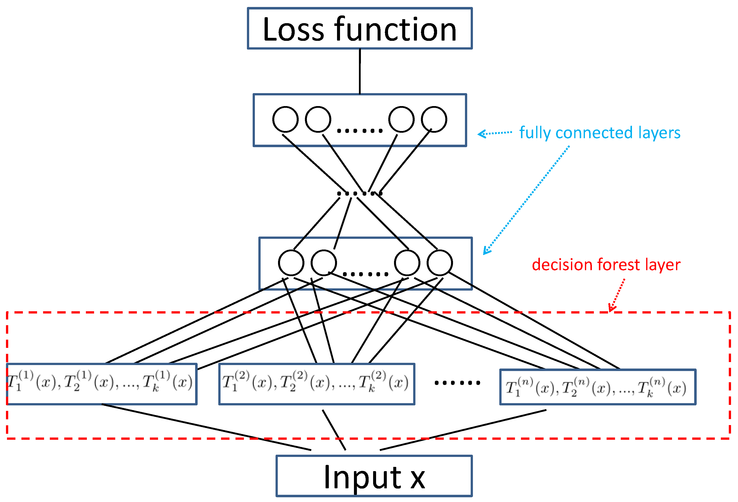
In this paper, we take a step forward to extend GBDT to a deep model. Specifically, we propose a deep architecture that combines GBDT with the multi-layer perceptron network [24]. As shown in Figure 1, from bottom to top, the proposed architecture has four parts: (1) The input data layer in which each data sample is represented by a vector; (2) The decision forest layer that consists of multiple hidden nodes. Each node is fitted by an ensemble of decision trees. This layer focuses on learning features from the input data. (3) Multiple fully connected layers, which focus on distilling knowledge from the decision forest layers. (4) The loss layer. For each node in the decision forest layer, we develop a GBDT-like method to generate a weighted sum of regression trees. Each tree is an estimated approximate gradient for an iteration, making the decision forest layer to compatible with back-propagation. Hence, the proposed deep architecture can be efficiently trained by stochastic gradient descent via back-propagation, which allows the proposed method to outperform tree ensemble methods. Compared with NN and the deep models based on convolutional networks or recurrent networks, the proposed method can select the useful numerical features when handling data without temporal/spatial structures. The learning task of DeepGBM is online prediction, which has to adapt the learning model to the online data generation, while it is not necessary to consider the new arrival data for the proposed method. There are a lot of models dedicated to solving concrete tasks, while our method is used for multiple tasks.
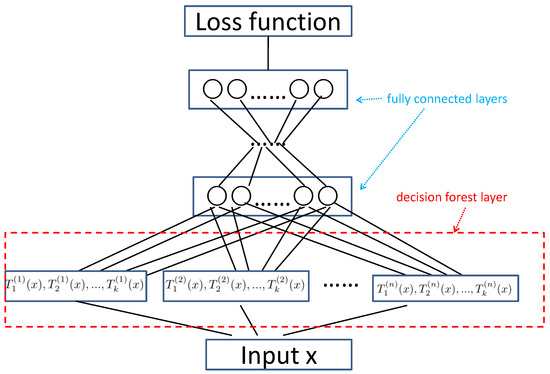
Figure 1.
Overview of the proposed architecture. From bottom to top, this architecture consists of four parts: (1) the input data layer; (2) the decision forest layer, which focuses on learning features from the input data; (3) multiple fully connected layers, which focuses on distilling knowledge from the decision forest layers; (4) the loss layer.
We conduct several experiments using eight datasets for multiple machine learning tasks, where four are used for a classification task, two are used for a regression task, and two are used for a ranking task. Comprehensive experimental results verified the effectiveness of the proposed architecture, e.g., it shows 2.22%, 2.16% and 5.60% increase against the corresponding second-best baseline on the Protein, Seismic and Isolet datasets, respectively. In summary, the fundamental contributions of this paper are listed as follows: (1) We propose an architecture based on GBDT and NN for multiple machine learning tasks, which could handle data without temporal/spatial structures. (2) We present a back-propagation procedure which will allow us to update the parameters by stochastic gradient descent. (3) We conduct empirical evaluations on several datasets for classification, regression, and ranking. The experimental results show that the proposed method can outperform the other methods.
The rest of this paper is organized as follows. We present the related work in Section 2 and present the different parts of the proposed architecture in Section 3. In Section 4, we present a back-propagation procedure to update the parameters by stochastic gradient descent for different machine learning tasks. All the experimental results are shown in Section 5. In Section 6, we present the complexity of the proposed architecture. Finally, we conclude our work in the Section 7.
2. Related Work
Random forest [16,17] is a widely used procedure which generates a number of regression or classification trees. Each tree is constructed by randomly selecting subsets of features. The results from the trees are aggregated to provide a prediction for each data, which leads to random forest providing higher accuracy in contrast with a single decision tree. Boosting is a successful technique for different machine learning problems, which was first proposed by Freund et al. in the form of the AdaBoost method [22]. This technique has been widely used in data analysis and real-world applications. AdaBoost uses decision trees as weak learners and integrates the decision trees into a strong classifier with the boosting technique. Recently, different machine learning systems have been proposed to train GBDT, e.g., XGBoost [26], LightGBM [27] and DimBoost [28].
It is worth noting that different models have been proposed [23,29,30] by combining tree ensemble methods and NN. Sethi [31] shows how to map a decision tree into a multi-layer perceptron network structure. Scornet et al. [29] show that each regression tree can be regarded as a particular multi-layer perceptron network and the random forest can be reformulated into a multi-layer perceptron network by restructuring several randomized regression trees as a collection of the multi-layer perceptron networks with particular connection weights. They first learn a random forest, and then extracted all the split directions and split positions to build the multi-layer perceptron network initialization parameters. Wang et al. [30] propose a novel model of decision-tree like the multi-layer perceptron network (NNRF), which has similar properties as a decision tree. Similar with random forest, NNRF has one path activated for each input, which leads it is efficient when performing forward and backward propagation. This technique also makes it easy to handle small datasets as the number of parameters is relatively small. NNRF learns complex functions when choosing the relevant paths of each node, which leads it outperforming random forest. Integrating GBDT and NN, Ke et al. [23] propose a learning framework DeepGBM for online prediction tasks. The framework consists of two parts: CatNN focuses on sparse categorical features and GBDT2NN focuses on handling dense numerical features. Powered by the above parts, this model has a strong learning capacity over numerical tabular features and categorical features while still having the ability to achieve efficient online learning.
3. Methodology
3.1. GBDT Algorithm
In this paper, we take a step forward by extending GBDT to a deep model. It is necessary to give the specific steps of GBDT. Given a training set , is a vector which represents the data point, is the predicted label. Each step is indicated as follows [20]:
Step 1: Compute the initial constant value by
where represents the loss function.
Step 2: The residual along the gradient direction is defined as
where n represents the number of iterations.
Step 3: By fitting the data into the initial model , we can construct a tree, where the parameter of the tree is based on the following expression as
Step 4: After minimizing the following loss function, we obtain the weight of the current model
Step 5: The new model is updated as
The residual of the former decision tree is the input for the next decision tree, which can reduce the residual, and the loss decreases following the negative gradient direction in each iteration. After n iterations, we will learn a model which consists of n decision trees. The final result is determined by the sum of results from all the decision trees.
3.2. Proposed Architecture
The proposed architecture is a deep neural network which consists of an input layer, a decision forest layer, multiple fully connected layers, and a loss layer. In this section, we will present these parts, respectively.
3.2.1. Input Layer
The motivation of the proposed architecture is to tackle the machine learning tasks whose data samples are represented by vectors with effective hand-crafted features, where each vector does not have any temporal/spatial structures. Hence, the input layer accepts data points in the form of vectors. We denote as the input layer.
3.2.2. Decision Forest Layer
The input layer is a decision forest layer, which is the crucial part of the proposed architecture and focuses on learning features from the input data. This layer consists of n hidden nodes, where each node is an ensemble of k decision trees. Specifically, we denote as the decision forest layer and as the output vector of the decision forest layer. For an input point x, the i-th () element in (i.e., the i-th hidden node in ) can be calculated by
where is the initial value of , () represents a regression tree, and s is a pre-defined shrinkage coefficient. The structure and parameters in each regression tree can by determined during the back-propagation process (see Section 4 for details).
3.2.3. Fully Connected Layers
On top of the decision forest layer, we construct multiple fully connected layers which are widely used in neural networks. The input of layer is the output of the decision forest layer. We denote , , …, as the fully connected layers on top of the decision forest layer. Suppose , are the input and output (after activation) of (. Then, we have the following:
where function represents the activation function and the matrix and the vector are the parameters in the i-th fully connected layer.
3.2.4. Loss Layer
On top of the last fully connected layer , we can define a loss layer for a specific machine learning task.
For classification, the output is , where K is the number of classes. Follow softmax [32], loss layer is defined by [33]:
where I is an indicator function and
The gradient is as follows:
For regression, square loss is used to define the loss layer:
The gradient is as follows:
For ranking, we use LambdaRank [21] to define the loss layer, which was based on RankNet [34] and directly optimizes Normalized Discounted Cumulative Gain (NDCG) [35]. NDCG is an evaluation metric and will be introduced later. Given a query set , the output is . The cost function of RankNet is as follows:
where is a parameter that determines the shape of the sigmoid and represents document , which ranks higher than . The gradient is
where
The LambdaRank’s key observation is that the costs themselves are unnecessary, except for the gradients. Following LambdaRank, we have
where is the size of change in metric NDCG by swapping the data point and . The gradient is as follows:
4. Optimization
Training the proposed architecture requires trying to find a solution to the parameters that minimizes the loss function. As shown in Algorithm 1, we present a back-propagation procedure to update these parameters by stochastic gradient descent.
| Algorithm 1 The back-propagation procedure for the proposed architecture |
Input: training set , maximal iteration number k, number n of hidden nodes in the decision forest layer, the shrinkage s. Output: 1. Initialize: and randomly initialize , by Gaussian distribution. 2. Repeat: forward propagation. 4. Update by Equation (20). 5. For , add a new tree to the ensemble of the i-th hidden node in the decision forest layer by Equation (22). 6. 7. Until . |
Since the fully connected layer is an easy studied component in neural networks, the parameters in the fully connected layers can be updated by stochastic gradient descent via back-propagation. Specifically, suppose
then we have:
and
where ⊙ represents the element-wise multiplication for matrices and is the learning rate.
In the decision forest layer, the regression trees in each of the n hidden nodes are constructed one by one. For each hidden node, we add one tree in an iteration of back-propagation. Specifically, in the p-th iteration of back-propagation , the negative gradient for the decision forest layer can be calculated as follows:
We denote as the i-th element in . Then, is the residual for the i-th hidden node in the decision forest layer. For a specific input x, we can obtain a residual . Then, for all of the training samples , we can obtain . After that, following the third step of GBDT [20], we construct a new regression tree by solving the problem . The ensemble of the tree in the i-th hidden node can be updated as follows:
where s is the shrinkage coefficient.
5. Experiments
We evaluate the proposed method (The source code has been released at https://github.com/dllinhe2017/Dgbdt, accessed on 1 January 2024) using several datasets for different tasks in this section. For classification, we compare the proposed method against the three most closely related baselines:
- GBDT [18], which consists of an ensemble of regression trees. It automatically selects the features with largest statistical information gain and combines the selected features to fit the training targets well when building trees.
- MLP [24], which makes up a number of interconnected processing elements and processes information by their dynamic state response to external inputs. We report the experimental results of two different models: and , where includes one hidden-layer and includes two hidden layers.
- NNRF [30], a novel model of decision-tree like the multi-layer perceptron network, which has similar properties to a decision tree (The author of NNRF only reported the experimental results for the classification task, so we neglected to select NNRF as the baseline method for the regression task). It has one path activated for each input.
For regression, we compare our method against two most closely related baselines: GBDT and MLP.
For ranking, we compare our method against the two most closely related baselines:
- Ranknet [34], which is a pair-based neural network method and learns the ranking functions by a probabilistic cost. Two sentences from the same document generated a pair and the label is determined by the scores of sentences.
- LambdaMART [21], which is based on Ranknet and directly optimizes NDCG. LambdaMART defines a weight parameter to represent the difference in NDCG when swapping a pair of documents. It is then used to update the weight in the next iteration.
5.1. Datasets
We evaluate the proposed methods and the baselines on four datasets for classification (https://www.csie.ntu.edu.tw/~cjlin/libsvmtools/datasets/multiclass, accessed on 21 January 2023) and two for regression (http://archive.ics.uci.edu/, accessed on 22 January 2023), respectively. The statistics information of these datasets is shown in Table 2. In particular, Isolet is a dataset that was used to predict which letter was spoken. Gesture is a dataset that was used to study gesture phase segmentation. The features of the datasets are hand-crafted and the structures of the datasets are not temporal/spatial.
Table 2.
Statistics information of the datasets for classification or regression.
For ranking, we use MQ2007 and MQ2008 (https://www.microsoft.com/en-us/research/project/letor-learning-rank-information-retrieval/letor-4-0/, accessed on 24 January 2023) to evaluate the proposed methods and the baselines. The statistical information is shown in Table 3.
Table 3.
Statistical information of the datasets for ranking.
5.2. Evaluation Metrics
For classification, we use the accuracy as the evaluation metric. Specifically, for a test set , let be the predicted class label of (), then let the accuracy rate be defined by
where is an indicator function that if the is false; otherwise, .
For regression, we use the Root of Mean Square Error (RMSE) as the evaluation metric. Specifically, for a test set , let be the predicted value of (), then let the RMSE be defined by
For ranking, we use NDCG and Mean Average Precision (MAP) [36,37] as the evaluation metrics. For a given set of search results, the Discounted Cumulative Gain (DCG) is
where T is a value representing the truncation level (usually less 10), and is the label of the ith listed URL. And the NDCG is defined by
MAP is defined by
where Q represents the number of queries,
where is the list’s precision at cut-off k. is also an indicator function. It is equal to 0 if the item at rank k is a irrelevant document, and is equal 1 otherwise, and is the number of relevant documents.
5.3. Experiment Settings
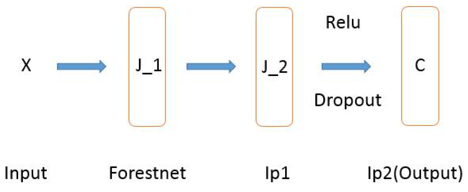
As shown in Figure 2, there are several parameters (the number of hidden nodes in forestnet is , the number of trees is K, and the number of hidden nodes in the fully connected layer is in the proposed model. The sensitivity of the three parameters will be analyzed in detail in Section 5.5.

Figure 2.
Structure of the proposed model for classification or regression tasks: (1) The decision forest layer (Forestnet) consists of hidden nodes. Each node has an ensemble of K. (2) The fully connected layer (Ip1) has hidden nodes. (3) The fully connected layer (Ip2) has C hidden nodes (for classification, C is the number of classes, and for regression, C = 1).
In the parameter tuning procedure for both the proposed and competitor methods, 10-fold cross validation is used. Note that no test data are involved in the parameter tuning. Given a training set, we divide it into 10 parts. One is chosen to be a validation set, while the remaining nine parts are used as the corresponding training set. The experiments are repeated 10 times and the 10 experiments are averaged to produce the best values of different parameters.
For all the classification tasks or the regression tasks, it is worth noting that the parameters and are chosen in the set by cross-validation. The parameter K is chosen in the set . The shrinkage rate is . We use ReLU as the activation function. The proposed model is trained by minibatch gradient descent, in which we set the learning rate to , the momentum to , and the weight decay to .
There are several parameters to set in the baseline algorithms. To ensure a fair comparison with the proposed model, it is worth noting that the parameter K in GBDT is chosen in the set by cross-validation; the parameter in MLP_1 is chosen in the set ; parameters and in MLP_2 are chosen in the set ; the number of layers d in NNRF is chosen in the set ; the parameter is chosen in the set by cross validation, the depth of regression trees is set to be 3.
For the ranking tasks, in the decision forest layer, the number of the hidden nodes is , each node has an ensemble of , and the shrinkage rate is . In the fully connected layer, the number of the hidden nodes is 12. Every fully connected layer uses maxout with a rate of . The proposed model is also trained by stochastic gradient descent, in which the learning rate is , the momentum is 0, and the weight decay is .
5.4. Results
Table 4 shows the comparison results for four datasets for classification tasks. We can observe that the proposed method shows superior performance gains over the baselines on the four datasets. Some statistics are listed below. For Gesture, the results of our method indicate a relative increase of 25.20% compared to the corresponding second-best baseline. The proposed method also shows 2.22%, 2.16% and 5.60% increase against the corresponding second-best baseline for the Protein, Seismic and Isolet datasets, respectively.
Table 4.
Comparison results with respect to the classification accuracy rate. On each dataset, 10 test runs were conducted and the average performance as well as the variance (numbers in parentheses) is reported.
Table 5 shows the comparison results on two datasets for regression tasks. We can observe that the proposed method performs better than the baselines. Next, we will list some statistics. The proposed method shows 54.52% and 0.97% decreases against the corresponding second-best baseline on the Slices dataset and YearPredictMSD dataset, respectively.
Table 5.
Comparison Results with respect to RMSE. On each dataset, 10 test runs were conducted and the average performance as well as the variance (numbers in parentheses) is reported.
Table 6 and Table 7 list the results for two datasets. For MQ2007, we can observe that our method outperforms RankNet and LambdaMART on all metrics. For MQ2008, we can also observe our method has superior performance gains over RankNet and LambdaMART on the metrics of NDCG@1 and mean NDCG, although it performs worse than LambdaMART on the metrics of NDCG@3 and MAP. The difference is negligible.
Table 6.
Comparison results for MQ2007. Ten test runs were conducted and the average performance, as well as the variance (numbers in parentheses), is reported.
Table 7.
Comparison Results on MQ2008. Ten test runs were conducted and the average performance, as well as the variance (numbers in parentheses), is reported.
5.5. Parameter Analysis
The most important parameters of the proposed framework are the number of hidden nodes in the decision forest layer, the number of trees K of each node, and the number of hidden nodes in the fully connected layer. We conduct experiments to investigate the effects on classification performances with different values of the three parameters. In the experiment, we use five-fold cross validation on the training data to set the parameters. Note that no test data are involved.
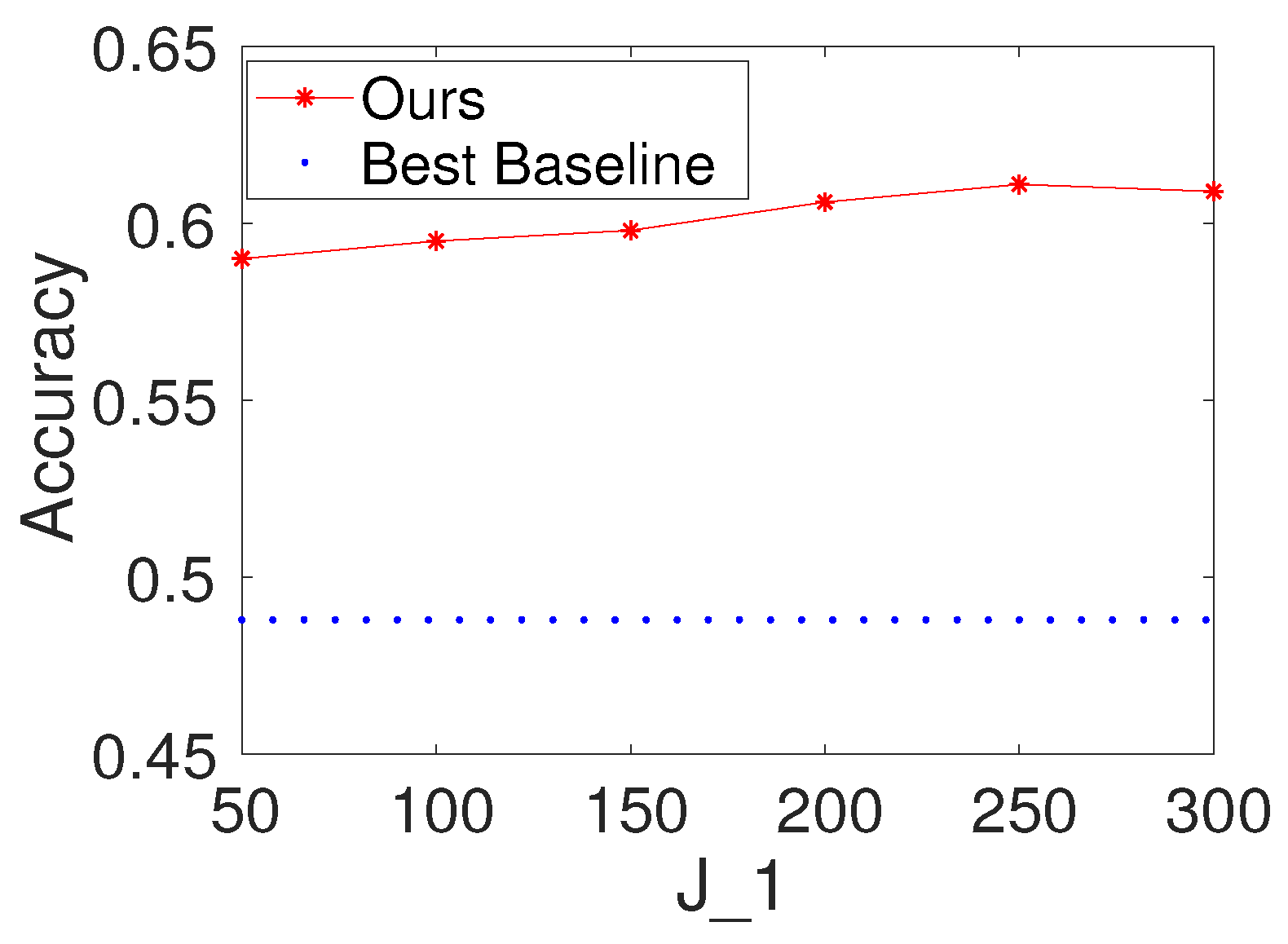
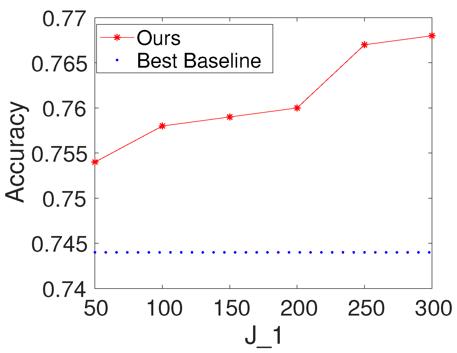
To investigate the effects of the number of hidden nodes in the decision forest layer, we first fix K and to be 100. We then vary the values of as . We report the results of the proposed method with different values of on Seismic and Protein. For comparison, we also provide the result of the best baseline. The results are shown in Figure 3 and Figure 4. Based on the figures, we make the following observations: (i) The performance of the proposed method is fairly good when is from 50 to 300. (ii) From the point of view of trade-offs between training cost and performance, it seems like a reasonable point when setting to be a value within . (iii) The performance of the proposed method increases a little on Seismic and Protein when is set to be bigger than 100.
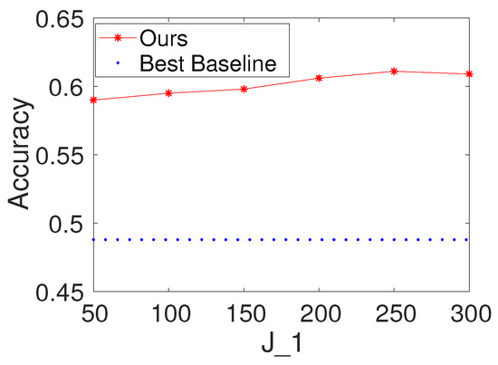
Figure 3.
Results with different values of the number of hidden nodes in the decision forest layer on Gesture (, ).
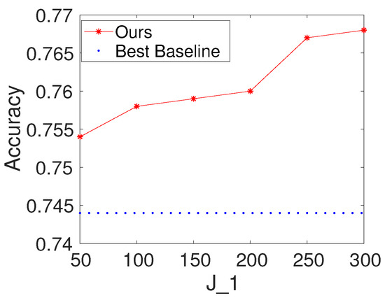
Figure 4.
Results with different values of the number of hidden nodes in the decision forest layer on Seismic (, ).
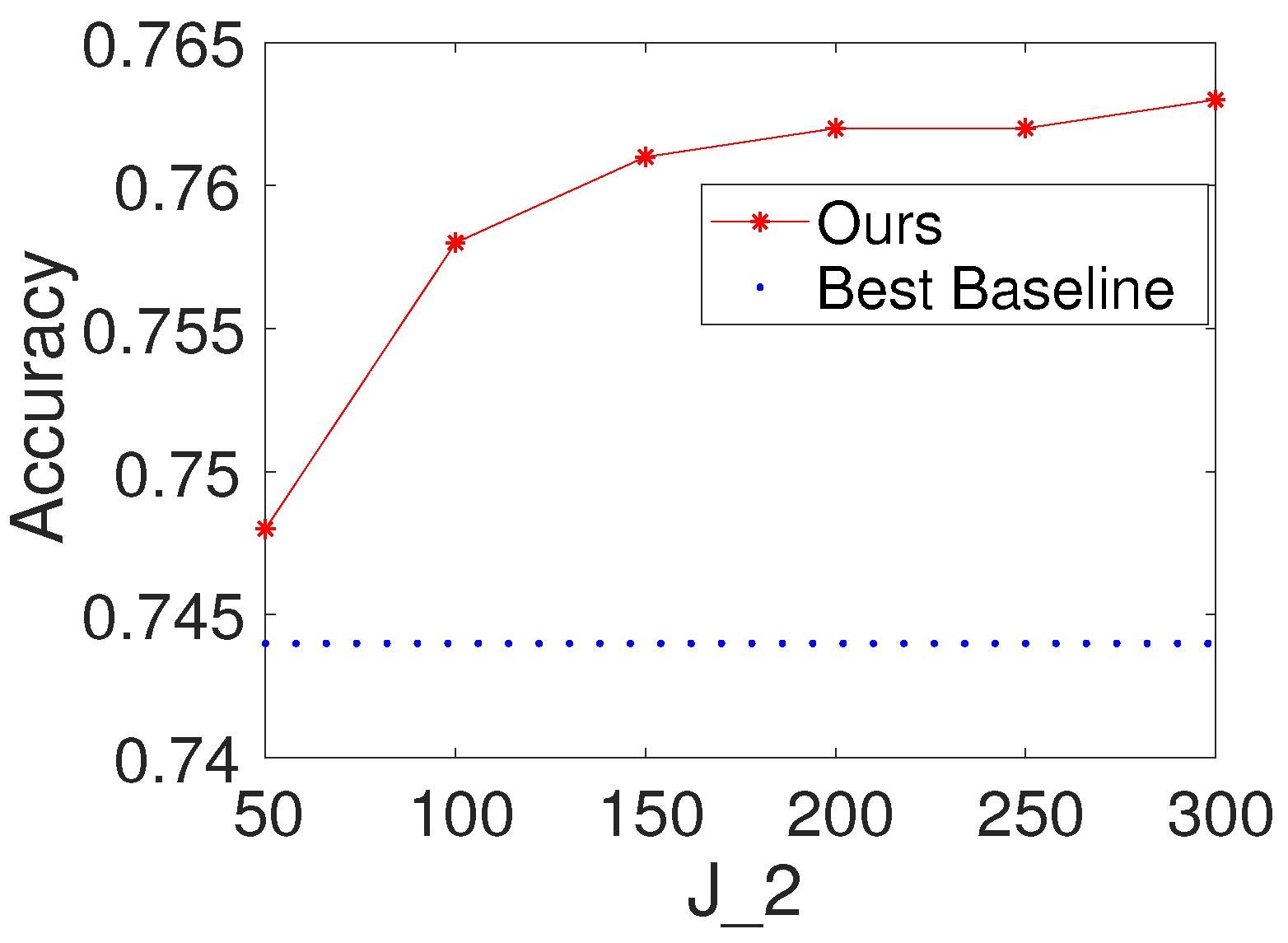
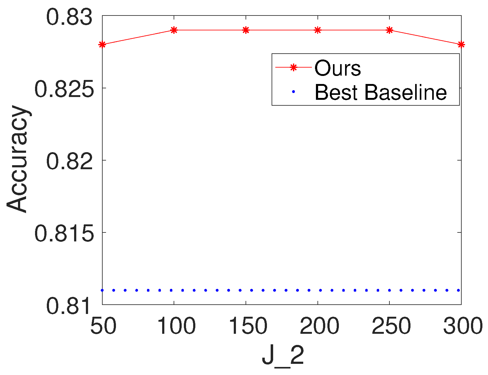
To investigate the effects of the number of hidden nodes in the fully connected layer, we first select K and to be 100. We then vary the values of as . We report the results of the proposed method with different values of for Seismic and Protein. For comparison, we also present the result of the best baseline. The results are shown in Figure 5 and Figure 6. Based on the figures, we make the following observations: (i) the performance of the proposed method is fairly good when is from 50 to 300; (ii) from the point of view of trade-offs between training cost and performance, it seems like a reasonable point when setting to be 100.
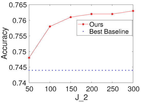
Figure 5.
Results with different values of the number of hidden nodes in the fully connected layer on Seismic (, ).
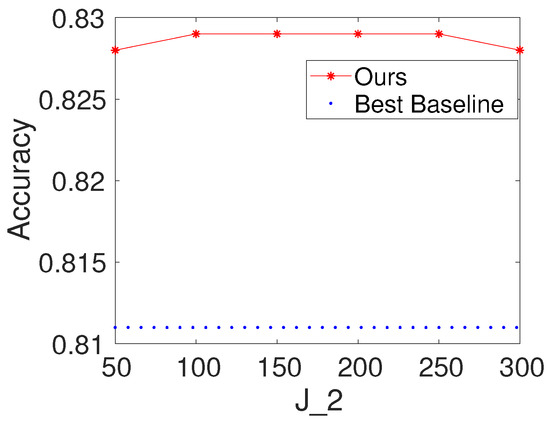
Figure 6.
Results with different values of the number of hidden nodes in the fully connected layer on Protein (, ).
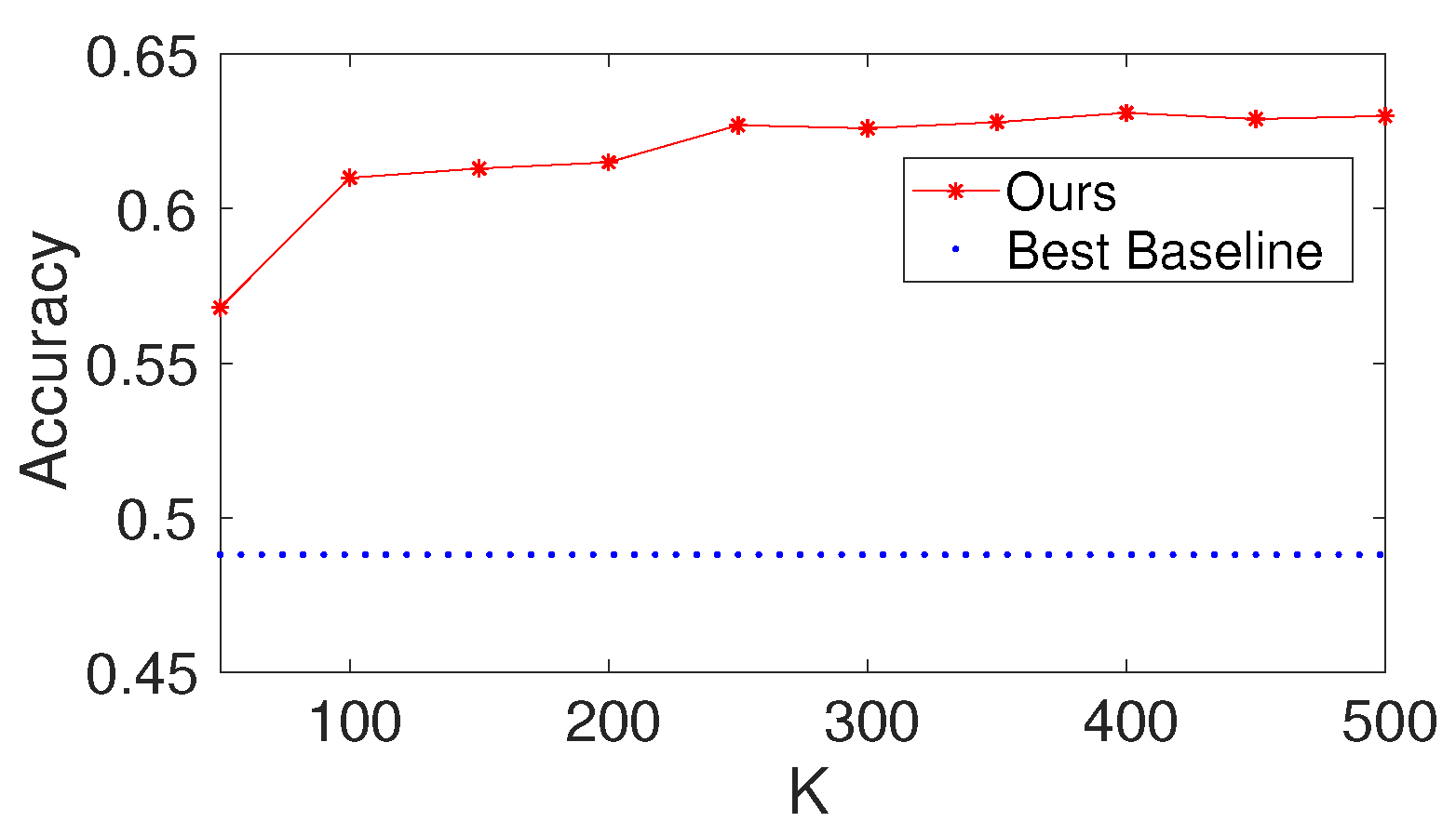
To investigate the effects of the number of trees K of each node in the decision forest layer, we first set and to be 100 and set the value of to be 50 to 500. We report the results of the proposed method with different values of K on Gesture. The results are shown in Figure 7. Based on the figure, we make the following observations: (i) the performance of the results increases at first and then increases a little; (ii) from the point of view of trade-offs between training cost and performance, it seems like a reasonable point when setting K to be 100.
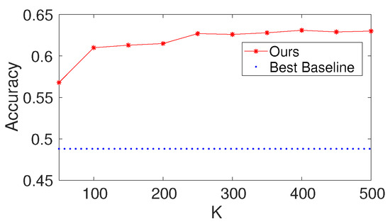
Figure 7.
Results with different values of the number of trees K of each node in the decision forest layer on Gesture (, ).
6. Complexity
The proposed method uses an architecture with a decision forest layer, followed by two fully connected layers and then the loss layer. Compared to GBDT, the proposed model has additional fully connected layers when the number of hidden nodes in the decision forest layer is set to be one. Compared to MLP, the proposed model has an extra decision forest layer.
7. Conclusions
The deep networks-based approaches do not work when handling data without spatial/temporal structures. To address this challenge, we propose a deep architecture that combines NN with GBDT, which takes advantage of GBDT’s ability to learn dense numerical features and NN’s strength in learning sparse categorical features by an embedding structure. Specifically, the architecture consists of two major parts: the decision forest layers focus on learning features from the input data and the fully connected layers focus on distilling knowledge from the decision forest layers. We designed an optimization procedure to train the proposed model via back-propagation. Although comprehensive experimental results verified the effectiveness of the proposed architecture, there are still some limitations: (1) it is not effective for all datasets, especially when learning datasets with sparse categorical features, because the experimental result is influenced by the specific context; (2) it has higher computational complexity in contrast to GBDT.
Author Contributions
Conceptualization, L.D. and S.D.; methodology, L.D. and S.D.; software, Y.X.; validation, Y.X., L.D. and S.D.; formal analysis, S.D.; investigation, H.S.; resources, H.S.; data curation, H.S.; writing—original draft preparation, Y.X. and H.S.; writing—review and editing, L.D. and S.D. All authors have read and agreed to the published version of the manuscript.
Funding
This research received no external funding.
Data Availability Statement
The data presented in this study are available in this article.
Conflicts of Interest
All authors were teachers of Taizhou University. They declare that the research was conducted in the absence of any commercial or financial relationships that could be construed as a potential conflict of interest.
References
- Khan, H.; Wang, X.; Liu, H. Handling missing data through deep convolutional neural network. Inf. Sci. 2022, 595, 278–293. [Google Scholar] [CrossRef]
- Zhou, S.; Deng, X.; Li, C.; Liu, Y.; Jiang, H. Recognition-Oriented Image Compressive Sensing With Deep Learning. IEEE Trans. Multimed. 2023, 25, 2022–2032. [Google Scholar] [CrossRef]
- Li, S.; Dai, W.; Zheng, Z.; Li, C.; Zou, J.; Xiong, H. Reversible Autoencoder: A CNN-Based Nonlinear Lifting Scheme for Image Reconstruction. IEEE Trans. Signal Process. 2021, 69, 3117–3131. [Google Scholar] [CrossRef]
- Rasheed, M.T.; Guo, G.; Shi, D.; Khan, H.; Cheng, X. An empirical study on retinex methods for low-light image enhancemen. Remote Sens. 2022, 14, 4608. [Google Scholar] [CrossRef]
- Rasheed, M.T.; Shi, D.; Khan, H. A comprehensive experiment-based review of low-light image enhancement methods and benchmarking low-light image quality assessment. IEEE Trans. Signal Process. 2023, 204, 108821. [Google Scholar] [CrossRef]
- Soleymanpour, M.; Johnson, M.T.; Soleymanpour, R.; Berry, J. Synthesizing Dysarthric Speech Using Multi-Speaker Tts For Dysarthric Speech Recognition. In Proceedings of the IEEE International Conference on Acoustics, Speech and Signal Processing, Singapore, 23–27 May 2022; pp. 7382–7386. [Google Scholar]
- Lu, H.; Li, N.; Song, T.; Wang, L.; Dang, J.; Wang, X.; Zhang, S. Speech and Noise Dual-Stream Spectrogram Refine Network With Speech Distortion Loss For Robust Speech Recognition. In Proceedings of the 2023 IEEE International Conference on Acoustics, Speech and Signal Processing (ICASSP), Rhodes Island, Greece, 4–10 June 2023; pp. 1–5. [Google Scholar]
- Liu, J.; Fang, Y.; Yu, Z.; Wu, T. Design and Construction of a Knowledge Database for Learning Japanese Grammar Using Natural Language Processing and Machine Learning Techniques. In Proceedings of the 2022 4th International Conference on Natural Language Processing (ICNLP), Xi’an, China, 25–27 March 2022; pp. 371–375. [Google Scholar]
- Collobert, R.; Weston, J. A unified architecture for natural language processing: Deep neural networks with multitask learning. In Proceedings of the 25th International Conference on Machine Learning, Helsinki, Finland, 5–9 July 2008; pp. 160–167. [Google Scholar]
- Collobert, R.; Weston, J.; Bottou, L. Natural language processing (almost) from scratch. J. Mach. Learn. Res. 2011, 12, 2493–2537. [Google Scholar]
- Asifullah, K.; Anabia, S.; Umme, C.Z.; Saeed, Q.A. A survey of the recent architectures of deep convolutional neural networks. Artif. Intell. Rev. 2020, 53, 5455–5516. [Google Scholar]
- Wang, X.; Gao, L.; Song, J. Beyond Frame-level CNN: Saliency-Aware 3-D CNN With LSTM for Video Action Recognition. IEEE Signal Process. Lett. 2017, 24, 510–514. [Google Scholar] [CrossRef]
- LeCun, Y.; Bengio, Y.; Hinton, G. Deep learning. Nature 2015, 521, 436–444. [Google Scholar] [CrossRef]
- Wang, F.; Tax, D.M. Survey on the attention based RNN model and its applications in computer vision. arXiv 2016, arXiv:1601.06823. [Google Scholar]
- Goodfellow, I.; Bengio, Y.; Courville, A. Deep Learning; MIT Press: Cambridge, MA, USA, 2016. [Google Scholar]
- Breiman, L. Random forests. Mach. Learn. 2001, 45, 5–32. [Google Scholar] [CrossRef]
- Díaz-Uriarte, R.; De Andres, S.A. Gene selection and classification of microarray data using random forest. BMC Bioinform. 2006, 7, 3. [Google Scholar] [CrossRef] [PubMed]
- Friedman, J.H. Greedy function approximation: A gradient boosting machine. Ann. Stat. 2011, 29, 1189–1232. [Google Scholar] [CrossRef]
- Mohan, A.; Chen, Z.; Weinberger, K. Web-search ranking with initialized gradient boosted regression trees. Proc. Learn. Rank. Chall. 2011, 14, 77–89. [Google Scholar]
- Rao, H.; Shi, X.; Rodrigue, A.; Feng, J.; Xia, Y.; Elhoseny, M.; Yuan, X.; Gu, L. Feature selection based on artificial bee colony and gradient boosting decision tree. Appl. Soft Comput. 2019, 74, 634–642. [Google Scholar] [CrossRef]
- Burges, C.J.C. From ranknet to lambdarank to lambdamart: An overview. Learning 2010, 11, 81. [Google Scholar]
- Freund, Y.; Schapire, R. A short introduction to boosting. In Proceedings of the Sixteenth International Joint Conference on Artificial Intelligence, San Francisco, CA, USA, 31 July–6 August 1999. [Google Scholar]
- Ke, G.; Xu, Z.; Zhang, J. DeepGBM: A deep learning framework distilled by GBDT for online prediction tasks. In Proceedings of the 25th ACM SIGKDD International Conference on Knowledge Discovery and Data Mining, Anchorage, AK, USA, 4–8 August 2019; pp. 384–394. [Google Scholar]
- Rosenblatt, F. The perceptron: A probabilistic model for information storage and organization in the brain. Psychol. Rev. 1958, 65, 86. [Google Scholar] [CrossRef] [PubMed]
- Paul, C.; Jay, A.; Emre, S. Deep neural networks for youtube recommendations. In Proceedings of the 10th ACM Conference on Recommender Systems, Boston, MA, USA, 15–19 September 2016; pp. 191–198. [Google Scholar]
- Chen, T.; Carlos, C. Xgboost: A scalable tree boosting system. In Proceedings of the 22nd ACM SIGKDD International Conference on Knowledge Discovery and Data Mining, San Francisco, CA, USA, 13–17 August 2016; pp. 785–794. [Google Scholar]
- Ke, G.; Meng, Q.; Finley, T.; Wang, T.; Chen, W.; Ma, W.; Ye, Q.; Liu, T.Y. Lightgbm: A highly efficient gradient boosting decision tree. Adv. Neural Inf. Process. Syst. 2017, 30, 3149–3157. [Google Scholar]
- Jiang, J.; Cui, B.; Zhang, C.; Fu, F. Dimboost: Boosting gradient boosting decision tree to higher dimensions. In Proceedings of the 2018 International Conference on Management of Data, Houston, TX, USA, 10–15 June 2018; pp. 1363–1376. [Google Scholar]
- Biau, G.; Scornet, E.; Welbl, J. Neural random forests. arXiv 2016, arXiv:1604.07143v1. [Google Scholar] [CrossRef]
- Wang, S.H.; Aggarwal, C.C.; Liu, H. Using a Random Forest to Inspire a Neural Network and Improving on It. In Proceedings of the 2017 SIAM International Conference on Data Mining, Houston, TX, USA, 27–29 April 2017; pp. 1–9. [Google Scholar]
- Sethi, I.K. Entropy nets: From decision trees to neural networks. Proc. IEEE 1990, 78, 1605–1613. [Google Scholar] [CrossRef]
- Boser, B.E.; Guyon, I.M.; Vapnik, V.N. A training algorithm for optimal margin classifiers. In Proceedings of the Fifth Annual Workshop on Computational Learning Theory, Pittsburgh, PA, USA, 27–29 July 1982; pp. 144–152. [Google Scholar]
- De Boer, P.T.; Kroese, D.P.; Mannor, S. A tutorial on the cross-entropy method. Ann. Oper. Res. 2005, 134, 19–67. [Google Scholar] [CrossRef]
- Burges, C.; Shaked, T.; Renshaw, E. Learning to rank using gradient descent. In Proceedings of the 22nd International Conference on Machine Learning, Bonn, Germany, 7–11 August 2005; pp. 89–96. [Google Scholar]
- Järvelin, K.; Kekäläinen, J. IR evaluation methods for retrieving highly relevant documents. In Proceedings of the 23rd Annual International ACM SIGIR Conference on Research and Development in Information Retrieval, Athens, Greece, 24–28 July 2000; pp. 41–48. [Google Scholar]
- Baeza-Yates, R.; Ribeiro-Neto, B. Modern Information Retrieval; ACM Press: New York, NY, USA, 1999. [Google Scholar]
- Ganjisaffar, Y.; Caruana, R.; Lopes, C.V. Bagging gradient-boosted trees for high precision, low variance ranking models. In Proceedings of the 34th International ACM SIGIR Conference on Research and Development in Information Retrieval, Beijing, China, 24–28 July 2011; pp. 85–94. [Google Scholar]
Disclaimer/Publisher’s Note: The statements, opinions and data contained in all publications are solely those of the individual author(s) and contributor(s) and not of MDPI and/or the editor(s). MDPI and/or the editor(s) disclaim responsibility for any injury to people or property resulting from any ideas, methods, instructions or products referred to in the content. |
© 2024 by the authors. Licensee MDPI, Basel, Switzerland. This article is an open access article distributed under the terms and conditions of the Creative Commons Attribution (CC BY) license (https://creativecommons.org/licenses/by/4.0/).