Abstract
Low-pressure discharge events have a major impact on a satellite’s electrical performance. Most notably, a number of serious issues arise from the inability to directly modify satellite systems that operate in orbit. Accurate analysis of electrical performance is crucial for mitigating the issues arising from the low-pressure discharge phenomenon. Complex structures, such as intricate features and curved structures, are frequently used in satellite systems’ enormous microwave components. In this case, the finite-difference time-domain (FDTD) approach proposes the hybrid implicit–explicit (HIE) algorithm with a domain decomposition method to effectively simulate complex structures under the low-pressure discharge phenomenon. The bilinear transform method is adjusted in accordance with the implicit equations for the anisotropic magnetized plasma environment caused by the discharge. To end unbounded lattices, a higher-order perfectly matched layer is used at the boundary. An example of a microwave connector structure is used to show how well the algorithm performs electrically. According to the findings, the suggested algorithm behaves in a way that is consistent with both the traditional algorithm and the experiments. Furthermore, the phenomenon of low-pressure discharge has a notable impact on the electrical performance of microwave components.
1. Introduction
One of the most important possible concerns when working in space is the discharge phenomenon, which has a major impact on the satellite system [1]. When the discharge phenomenon occurs, the satellite system experiences disconnected, uncontrollable, or even catastrophic failure. Low-pressure discharge and multipactor discharge are two types of discharge phenomena [2]. In contrast to multipactor discharge, low-pressure discharge takes place at pressures ranging from 1.3 Pa to 1000 Pa. Up till now, the multipactor phenomenon and the discharge mechanism have received the majority of research attention [3,4,5]. Most studies mainly investigated the theoretical solution of the Paschen curve. Through the calculation of the Paschen curve, the reaction between material and air under high-power excitation and low pressure can be revealed. However, these investigations can only solve ideological problems, which has significant limitations in practical engineering. In order to resolve such conditions, the majority of research up to this point has looked at discharge thresholds and experimental techniques [6,7]. Practical engineering might greatly benefit from an effective way to quantitatively assess electrical performance in order to forecast the discharge occurrence and modify the system in space.
The extraordinarily high power ionizes the gas inside the discharge-sensitive area when the low-pressure discharge phenomenon occurs. A plasma environment is created as a result [3]. To effectively convey the microscopic features, the anisotropic magnetized plasma model is taken into consideration [8]. Magnetized plasma has a distinctive anisotropic behavior in the presence of an external magnetic field. The electrical performance is greatly altered when magnetized plasma forms [9]. Therefore, the two main issues are precisely simulating the plasma characteristics and electronic behavior. The full-wave simulation method can be immediately connected to the computational fluid dynamics (CFD) method to derive the plasma parameters [10]. As of right now, a few techniques for simulating anisotropic magnetized plasma have been established based on the finite-difference time-domain (FDTD) algorithm, which exhibits notable accuracy and efficiency [11,12,13,14].
One of the most vulnerable regions for low-pressure discharge is the connections between various components [15]. The efficiency of the conventional method is impacted by the large number of small features in the connector construction that cause a multiscale problem to arise. The smallest details determine the traditional algorithm’s correctness and efficacy. Stated differently, the mesh size needs to be selected with sufficient precision to guarantee the algorithm’s efficacy and precision. The reason is because the Courant–Friedrich–Levy (CFL) condition limits the stability of the time-explicit conventional FDTD algorithm [16]. Nevertheless, in multiscale issues, an unacceptably long simulation time is caused by an excessively tiny mesh size. The simulation results will become erroneous or perhaps fail if the mesh size increases to the point where the CFL condition is not satisfied. Unconditionally stable algorithms, such as split-step (SS), locally one-dimensional (LOD), alternative direction implicit (ADI), and others, are presented to alleviate such situations and preserve significant accuracy while overcoming the CFL condition [17,18,19]. While unconditionally stable algorithms are capable of preserving algorithmic stability in the absence of stability condition limitations, their efficiency is limited to specific details across all dimensions [20]. The hybrid implicit–explicit (HIE) technique is presented to solve fine details only along low dimensions in order to achieve a significant performance for low-dimensional fine details [21]. Time steps can be increased in accordance with the use of the HIE algorithm with a significant degree of accuracy by using the implicit updating procedure. The original HIE method performs degeneration of conformal structures with uniform mesh selection behaviors. The domain decomposition (DD) method is used to increase the computation accuracy in fine details with conformal structures [22]. Mesh size can be selected using the DD approach in accordance with the calculation requirements.
At the domain boundaries, absorbing boundary conditions have to be used in order to simulate open-area issues in limited space. One of the most effective absorbing boundary conditions is the perfectly matched layer (PML) formulation [23]. Six auxiliary variables based on the split-field method are added to the original PML formulation, which causes efficiency and absorption to degenerate. To help with this issue, unsplit-field techniques like stretch coordinate (SC) and complex frequency-shifted (CFS) schemes are introduced [24,25]. Reduced late-time reflections and the absorption of low-frequency evanescent waves are two benefits of unsplit-field systems [26]. Low-frequency propagation waves, however, cannot be effectively absorbed by these systems. When there are several low-frequency outgoing waves in a problem, this condition makes the computation erroneous. A higher-order PML formulation is used to address this issue, and it is accomplished by multiplying the stretched coordinate variables by one to create a single term [27]. The length and resource requirements of the simulation increase with the application of higher-order PML schemes. In order to mitigate this situation, a higher-order PML method that uses the unsplit-field formulation is used to lower the computing complexity of an algorithm that retains four auxiliary variables while updating each Maxwell’s equation [28]. Up to now, the HIE algorithm has changed to a higher-order formulation in response to various situations.
One of the most sensitive low-pressure discharge locations is the connector structure, which connects the microwave’s component parts. Despite the introduction of certain pertinent works utilizing the HIE algorithm for plasma simulation, these efforts remain insufficient in effectively assessing the electrical performance of microwave connector structures during low-pressure discharge events. The following is a description of the primary drawback: (1) One of the most significant components of huge microwave components are curve structures. Conventional structures cannot be solved effectively by using current methods. A significant impact on computation accuracy will result from directly using an existing algorithm. (2) Magnetized plasma with anisotropic characteristics that can effectively reflect the microscopic property is created when a discharge occurs. Large calculation errors will arise at the intersection of curves and boundaries when magnetized plasma is calculated directly using pre-existing techniques. As such, a different approach ought to be taken into account. (3) It should be noticed that the conventional FDTD algorithm is discretized based on the cubic Yee grid. Such a condition results in a large calculation error with curve structures. Meanwhile, in order to maintain the accuracy of the algorithm, the chosen mesh size must be fine enough, which results in significant decrements in efficiency. Thus, the DD method shows advantages in curve structures and extremely fine local structures.
In this paper, a domain decomposition HIE algorithm is proposed for the low-pressure discharge phenomenon. A microwave connector is employed as an example for demonstration. From the results, it can be concluded that the proposed algorithm can accurately analyze electrical performance with the low-pressure discharge phenomenon. The novelty of this paper can be summarized as follows: (1) For the anisotropic magnetized plasma, an alternative method for the implicit scheme is modified based on the HIE algorithm with considerable accuracy. (2) A higher-order perfectly matched layer formulation is employed for the termination of boundaries to absorb outgoing waves. (3) The domain decomposition method is modified to simulate conformal structures based on the HIE algorithm.
2. Formulation
In this section, the implementation of the domain decomposition HIE algorithm inside the plasma environment is demonstrated. At the sensitive area, anisotropic magnetized plasma is produced as a result of the low-pressure discharge phenomenon. As a result, an anisotropic magnetized plasma computational domain is used. The magnetized plasma’s Maxwell’s equations inside the PML areas are given by
where represents the polarization current density of the magnetized plasma, is the frequency, and and are the relative permittivity and relative permeability. is the Laplacian operator which can be given as
where is the stretched coordinate variables with the higher-order scheme which can be given as
where , is assumed to be positive real, while and are assumed to be real. According to the partial fraction method, stretched coordinate variables can be given as
where the coefficients are , , and . In order to clearly demonstrate this, the proposed algorithm is divided into several parts in the following part.
2.1. Discretization in FDTD Domain
Similar methods can be used to determine the electric and magnetic components through the symmetry of the Maxwell’s equations. As a result, , , and components are used as examples throughout the demonstration. One can obtain Maxwell’s equations by utilizing the individual component’s form.
By substituting (2c) into (3a) and (3b), the results can be given after introducing auxiliary variables as
where the introduced auxiliary variables can be given as, for example,
By transforming (4a,b) into the time domain according to the Fourier transform, the results can be given as
According to a similar approach, auxiliary variables can be given as
2.2. Solution in the Higher-Order PML Regions
Assuming the existence of fine details along the y-direction, the components are explicitly calculated along that direction. Equations (6a,b), as a result of the stepping of the HIE algorithm, can be represented as
where is the first-order finite-difference form given as, for example,
The auxiliary variables are manipulated as
where the coefficients can be given as
By substituting auxiliary variables (9a) and (9b) into (8a), the results can be given as
where the coefficients are and .
2.3. Employment of HIE Algorithm
It can be observed that the and components are coupled, so they cannot be updated directly. To alleviate such a condition, is substituted into for decoupling, given as
A tridiagonal matrix that can be implicitly renovated is generated at the left side by (11). The field components are dissociated in accordance with the HIE algorithm, as can be seen from (11). The electric current density is still dissociated from the field components along the x-direction though. An alternate technique for calculating magnetized plasma is required to alleviate such a situation. For instance, the magnetized plasma’s constitutive relationship is given as
where , , and represent the plasma frequency, electron gyrofrequency, and damping constant, respectively. It is observed that and are coupled, which results in non-updated equations. According to the auxiliary differential equation (ADE) method, Equation (12) is given as
Through (13), it can be observed that the equations are modified according to the HIE algorithm. By substituting into (13) to decouple the equations, the results are given as
where , , , , , , and . At each time step, they should be updated simultaneously because the electric current density is connected. The simultaneous solution can be used to derive the whole algorithm by replacing (14) with (11), as follows:
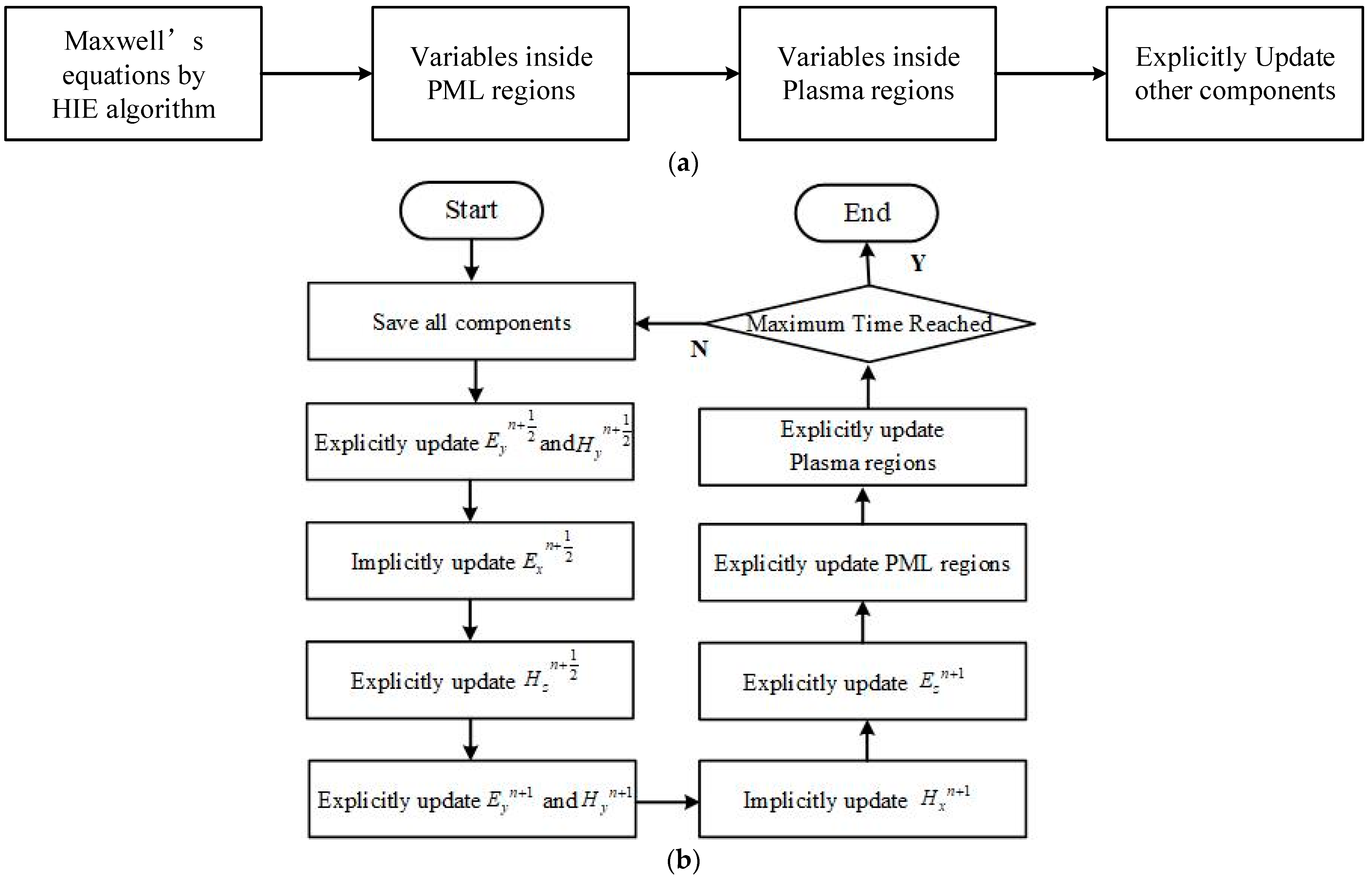
The solution of the entire algorithm can be summarized by the following procedure, as shown in Figure 1a, which includes (1) Maxwell’s equations in the FDTD domain by using the HIE algorithm; (2) updated variables inside the PML regions; (3) updated variables in the magnetized plasma; (4) explicitly updated variables and coefficients. The updating procedure of the individual components is shown in Figure 1b.

Figure 1.
(a) Solution of entire algorithm; (b) updating procedure of individual components.
3. Solution of Domain Decomposition in Non-Uniform Domains
Conformal manipulation is required due to the local exceedingly small features and curve structures, which results in erroneous calculations. While choosing a finer mesh size will increase the accuracy of the calculation, the total cost of the calculation will increase significantly or may even become undesirable. The DD technique is brought into the FDTD domain to alleviate such a situation. Nevertheless, the simulation will be rendered invalid if the suggested technique is implemented using the current DD approach directly. As a result, an alternate DD technique for the suggested algorithm is proposed below.
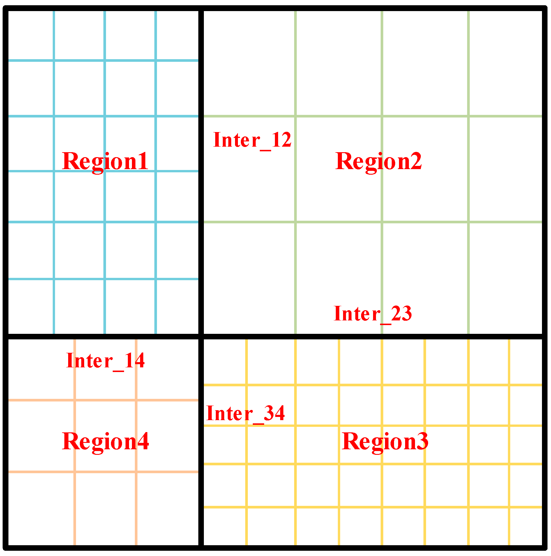
The four sub-regions of the uniform computational domain including regions 1, 2, 3, and 4 are depicted in Figure 2. Interfaces, such as Inter_12, Inter_14, Inter23, and Inter_34, connect various sub-regions. The original implicit equation in the HIE method, as per Equation (15), can be expressed as
where represents the matrix at the left side of (16), while , , and represent the components at a time step of n, n − ½, and n − 1. In the sub-regions, Equation (16) can be written as

Figure 2.
The uniform computational domain with four sub-regions.
The results can be obtained by expanding (18) into the form of individual components and replacing the components at the interfaces with those inside the sub-regions.
It is evident that the left side of (18) forms the Schur complement, which is explicitly solvable. By solving field components at the interfaces, one may correspondingly solve field components inside the sub-regions using Equation (17).
It should be noticed that the conventional FDTD algorithm is discretized based on the cubic Yee grid. Such a condition results in a large calculation error with curve structures. Meanwhile, in order to maintain the accuracy of the algorithm, the chosen mesh size must be fine enough, which results in significant decrements in efficiency. Thus, the DD method shows advantages in curve structures and extremely fine local structures.
4. Numerical Example
The effectiveness of the proposed algorithm is demonstrated through the microwave connector model. One of the most prominent space phenomena that has a big impact on system performance is the discharge. Additionally, under specific conditions, the discharge phenomenon frequently happens at the microwave connecting structure. As a result, the simulation of the structure of microwave connectors under discharge phenomena has significant implications for satellite systems. This section not only offers a different approach to the quantitative analysis of electric behavior during low-pressure discharge phenomena, but it also shows how successful the suggested algorithm is. It is mentioned that the microwave connector is composed of curves and fine local details. In such circumstances, the proposed DD method shows advantages in memory consumption and calculation efficiency.
4.1. Model Demonstration of Microwave Connector Structure
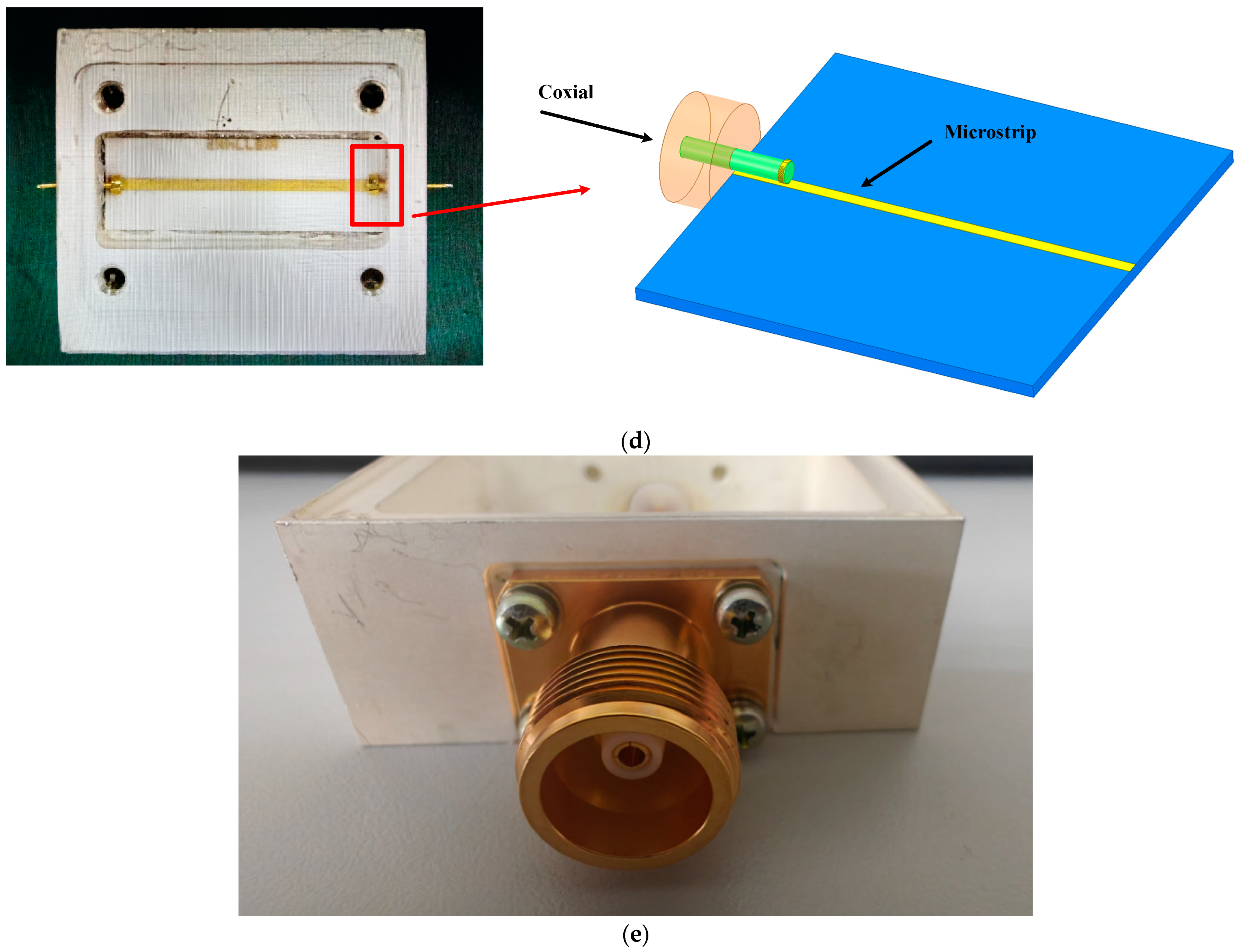
This section uses a microwave connector structure made of metal and dielectric material. It joins the coaxial cable and microstrip. The microstrip, coaxial cable, metal ribbon, and dielectric substrate make up the whole structure. The parameters of the dielectric substrate and outer coaxial cable are and , respectively. The detailed parameters of the microwave connector structure are shown in Table 1. The microwave connector structure’s front, side, and top views are displayed in Figure 3. Figure 3d also displays the physical photo of the microwave connector model. The simulation structure represents one of the ports.

Table 1.
The parameters of the microwave connector structure.
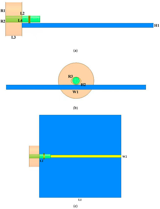

Figure 3.
The front view, side view, and top view of the microwave connector structure: (a) front view; (b) side view; (c) top view; (d) the entire structure and its physical photo; (e) a physical photo of the microwave connector.
4.2. Analyzation of Magnetized Plasma Occurring due to Low-Pressure Discharge Based on CFD Method
It can be observed that with the circumstance of 5 mbar, low-pressure discharge occurs with a power of 108 W. Such a circumstance can be regarded as the most significant working condition. Thus, the wave excitation of the model is selected as 108 W. The parameters of the anisotropic magnetized plasma are obtained under 5 mbar.
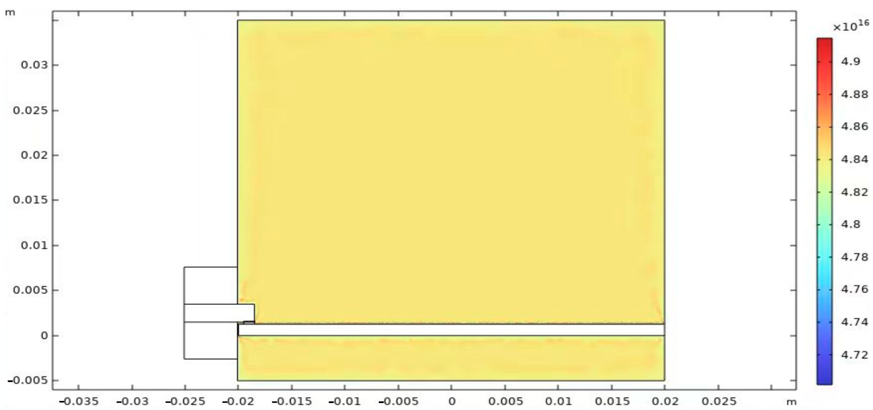
In such circumstances, the parameters and distribution of the anisotropic magnetized plasma and electric density can be obtained according to the CFD simulation, as shown in Figure 4a–d. Figure 5 shows the simulation results obtained by the CFL simulation. The results show that at a pressure of 5 mbar and an excitation of 108 W, the low-pressure discharge phenomenon occurs at the sensitive area. Anisotropic magnetized plasma is formed in the low-pressure discharge area in such circumstances, as shown in Figure 4. The parameters of the magnetized plasma can be obtained as rad/s, rad/s, and Hz. Furthermore, the proposed algorithm can still evaluate the microwave components without the discharge phenomenon, which can be implemented by filling the computational domain with a vacuum.
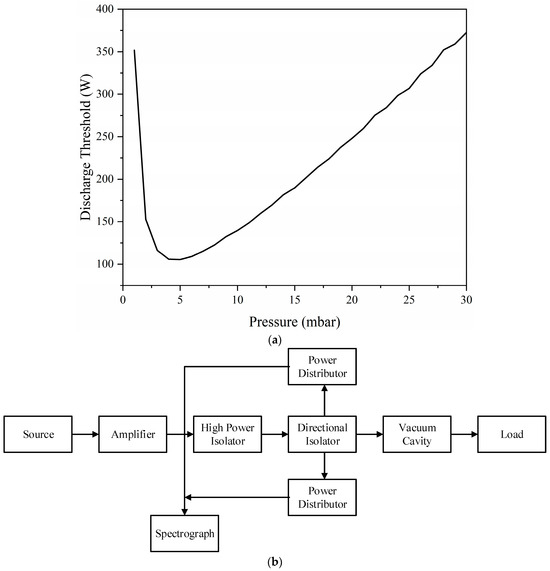

Figure 4.
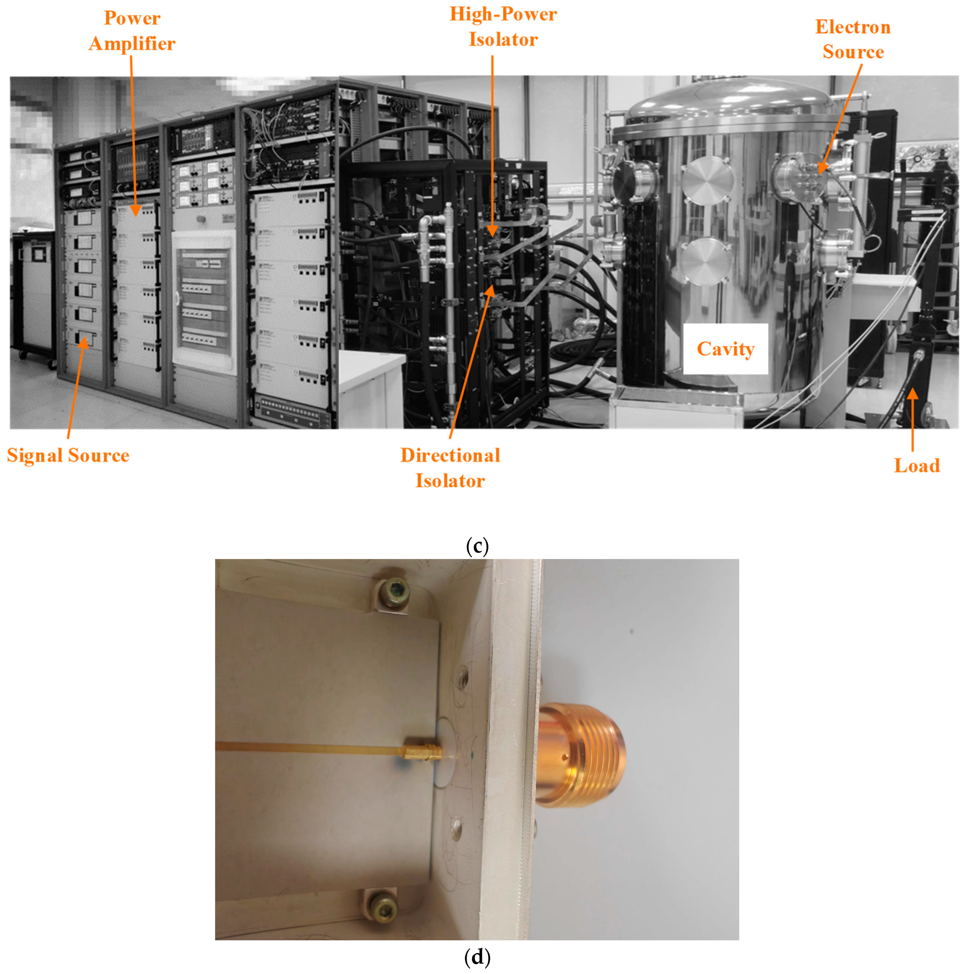
(a) The relationship between the pressure and discharge thresholds. (b) A diagram of the experimental system. (c) The experimental environment. (d) The excitation source of the microwave connector.

Figure 5.
The distribution of the electric density of the microwave connector structure.
As shown in the experiment, the relationship between the pressure and discharge thresholds can be obtained from Figure 4a. The experimental environment is shown in Figure 4b. The excitation source of the microwave connector is shown in Figure 4c,d. The model is located inside the cavity and excited by the plane wave.
4.3. Demonstration of Proposed Algorithm including Higher-Order PML Scheme, HIE Procedure, and DD Method
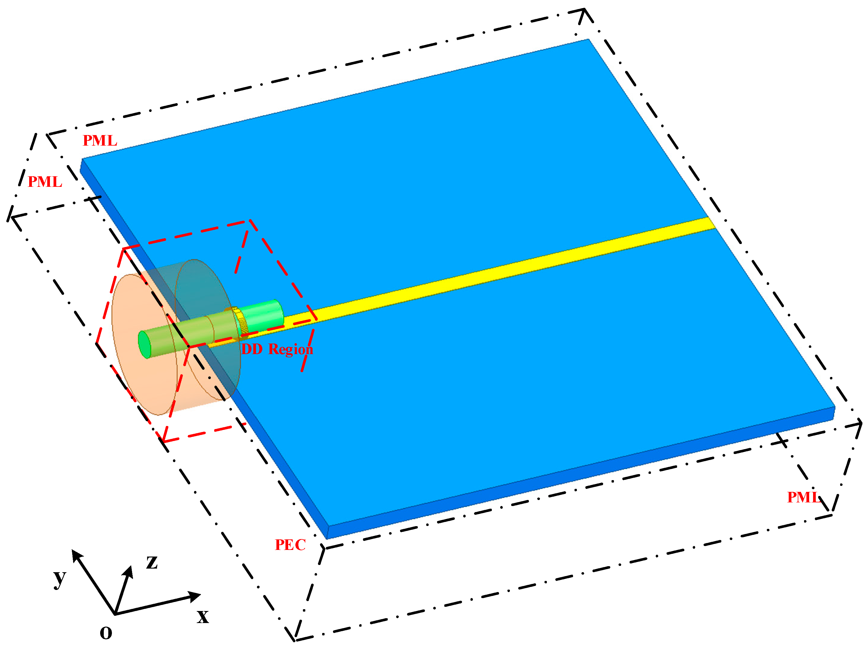
The computational domain is shown in Figure 6. The plane wave, which is the same as in the experiment above, propagates along the positive x-direction. The modulated Gaussian wave with a maximum frequency of 2 GHz and a center frequency of 1 GHz is the incidence wave. The perfect electronic conductor (PEC) ends at the left border. Ten-cell PML regions end at the remaining boundaries. The parameters are selected inside the PML zones to achieve the best results in the frequency and temporal domains.

Figure 6.
A sketch picture of the microwave connector structure’s computational domain.
The entire computational domain holds the dimensions of mm. The structure is located at the center of the domain. To improve the accuracy of the calculation, the DD region contains the entire coaxial region with the dimensions of mm. It can be observed that the entire structure holds extremely fine details along the vertical z-direction. Thus, the mesh size along the z-direction is chosen as mm. The mesh sizes of the x- and y-directions are mm. The mesh size in the DD region is mm.
The maximum time step of the conventional explicit algorithm can be obtained as fs. The maximum time step of the HIE algorithm can be obtained as fs, whose maximum CFL number (CFLN) corresponds to 3.4. The CFLN is defined as , where is the time step of the implicit algorithm.
In order to demonstrate the effectiveness of the algorithm, algorithms without the DD method are also introduced for the illustration which include the FDTD-PML in [29], the original HIE-PML in [30], and the proposed HIE-HPML. Meanwhile, the FDTD-PML with an extremely fine mesh size which holds mm is chosen for comparison, denoted as FM-FDTD-PML. To simplify the demonstration, the proposed algorithm with the DD method is denoted as DD-HIE-HPML. Thus, through comparisons between the different conventional algorithms and the proposed DD scheme, the effectiveness of the DD algorithm can be demonstrated.
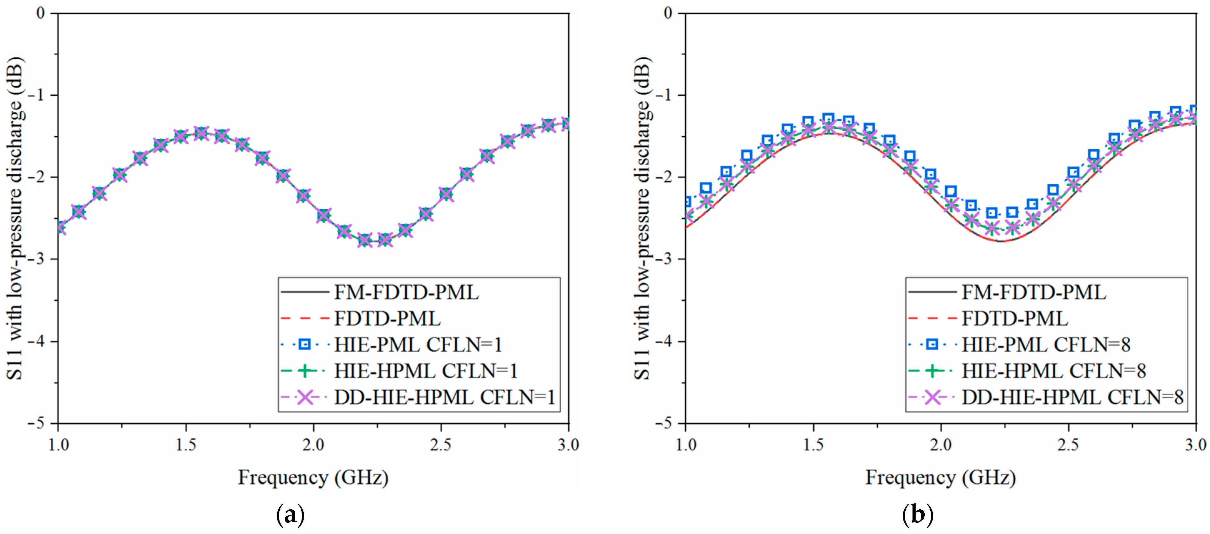
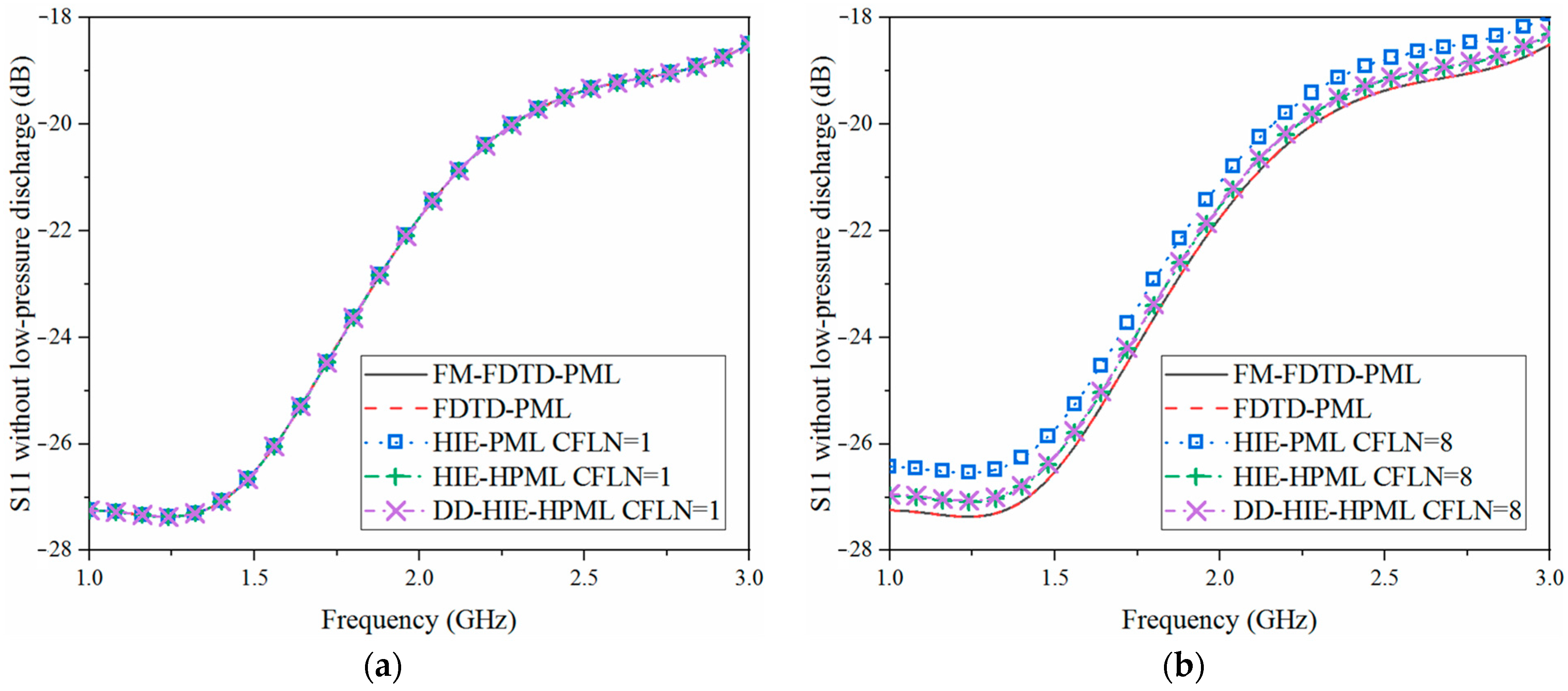
Figure 7 shows the return loss (S11) parameters obtained by using different PML algorithms with the low-pressure discharge phenomenon. Figure 8 displays the return loss (S11) obtained by using different PML algorithms without the low-pressure discharge phenomenon. As shown in Figure 7a and Figure 8a, it can be observed that the curves are overlapped. The reason is that all of these algorithms hold the same calculation accuracy with a lower time step. As shown in Figure 7b and Figure 8b, the curves show shifting compared with the results obtained by using a lower time step. The rationale is that an increase in the time step causes a corresponding increase in the numerical dispersion. The calculation accuracy deteriorates under such circumstances. The suggested approach has the highest accuracy among these implicit algorithms with the largest time step; this accuracy is nearly identical to that of the FM-FDTD-PML. Comparing the algorithm using the DD approach to the one without, the latter can achieve the same performance. This condition suggests that the suggested algorithm is accurate and efficient. As seen in Table 2, the algorithm’s effectiveness can also be seen in memory usage, simulation duration, and time decrease with various CFLNs.

Figure 7.
The return loss (S11) parameter obtained by using different PML algorithms with the low-pressure discharge phenomenon: (a) CFLN = 1; (b) CFLN = 8.

Figure 8.
The return loss (S11) parameter obtained by using different PML algorithms without the low-pressure discharge phenomenon: (a) CFLN = 1; (b) CFLN = 8.
Table 2.
Memory consumption, simulation duration, and time reduction by different algorithms and CFLNs.
Because matrices are implicitly calculated for each time step, it is evident that implicit methods need more memory. The situation can be mitigated by augmenting the CFLNs, whose duration is markedly extended under such conditions. Even if the FDTD-PML and FM-FDTD-PML can achieve the same calculation accuracy, the increasing mesh numbers cause a large rise in memory usage and simulation length with extremely tiny mesh sizes. The suggested algorithm performs better than the other implicit algorithms in terms of efficiency and memory as a result of the DD technique. Such a requirement suggests that both the efficiency and memory consumption of the suggested algorithm are effective. It is evident from Figure 7 and Figure 8 that there are large differences in the return loss when there is a low-pressure discharge phenomenon. Such a circumstance suggests that the microwave device’s electrical performance is impacted by the presence of magnetized plasma during a low-pressure discharge event. A situation like this causes the system to malfunction or perhaps behave degenerately.
5. Conclusions
Here, the DD method and the HIE algorithm with a higher-order perfectly matched layer are suggested for evaluating the electrical performance of low-pressure discharges. The suggested algorithm exhibits benefits in relation to anisotropic magnetized plasma, curve shapes, and single-direction extremely fine details. Using a numerical example, the suggested methodology is shown to be in accord with the traditional explicit method as well as stable in the modeling of anisotropic magnetized plasma caused by the low-pressure discharge phenomenon. It has advantages over the original HIE approach in terms of accuracy, efficiency, and memory usage. By cutting down on the number of mesh sizes, the DD approach can dramatically reduce both the amount of memory used and the length of the simulation. Most notably, it can demonstrate how low pressure has a substantial impact on a microwave device’s electrical performance. Such a situation causes the system’s performance to deteriorate or maybe fail completely while in space.
Author Contributions
Conceptualization, W.C.; Data curation, R.W.; Formal analysis, W.C. and L.Z.; Funding acquisition, R.W.; Investigation, H.W.; Methodology, W.C., R.W.; Project administration, L.Z.; Resources, W.C.; Software (Comsol 5.4), R.W.; Validation, Y.W.; Writing—original draft, R.W. and W.C.; Writing—review & editing, W.C., R.W. All authors have read and agreed to the published version of the manuscript.
Funding
This study was funded by the National Key Laboratory Foundation 2022-JCJQ-LB-006 (6142411132202) and the National Natural Science Foundation of China (62301013, 61571022, 61971022).
Data Availability Statement
The data are only available on request due to restrictions, e.g., privacy or ethical reasons.
Conflicts of Interest
The authors declare no conflicts of interest.
References
- Arentsen, M.T.; Bak, C.L.; da Silva, F.F.; Lorenzen, S. External Partial Discharge Analysis in Design Process of Electrical Space Components. In Proceedings of the 2019 European Space Power Conference (ESPC), Juan-les-Pins, France, 30 September–4 October 2019; pp. 1–5. [Google Scholar] [CrossRef]
- Yang, Z.; Yang, Z.; Xia, H.; Lin, F. Brake Voltage Following Control of Supercapacitor-Based Energy Storage Systems in Metro Considering Train Operation State. IEEE Trans. Ind. Electron. 2018, 65, 6751–6761. [Google Scholar] [CrossRef]
- Wang, L.; Liao, C.; Ding, D.; Gao, J. Numerical Study on Low Pressure Discharge of Microwave Stepped Impedance Transformer. In Proceedings of the 2023 International Applied Computational Electromagnetics Society Symposium (ACES-China), Hangzhou, China, 15–18 August 2023; pp. 1–3. [Google Scholar] [CrossRef]
- Berenguer, A.; Coves, Á.; Mesa, F.; Bronchalo, E.; Gimeno, B. A New Multipactor Effect Model for Dielectric-Loaded Rectangular Waveguides. In Proceedings of the 2019 IEEE MTT-S International Conference on Numerical Electromagnetic and Multiphysics Modeling and Optimization (NEMO), Boston, MA, USA, 29–31 May 2019; pp. 1–4. [Google Scholar] [CrossRef]
- Zhang, L.; Wang, H.; He, S.; Wei, H.; Li, Y.; Liu, C. A Segmented Polynomial Model to Evaluate Passive Intermodulation Products from Low-Order PIM Measurements. IEEE Microw. Wirel. Compon. Lett. 2019, 29, 14–16. [Google Scholar] [CrossRef]
- Ren, H.; Xie, Y. Simulations of the Multipactor Effect in Ferrite Circulator Junction with Wedge-Shaped Cross Section Geometry. IEEE Trans. Electron Devices 2020, 67, 5144–5150. [Google Scholar] [CrossRef]
- Zhang, X.; Yu, Q.; Ni, X. Saturation Mechanism of Multipactor Effect in a One-Sided Dielectric-Loaded Waveguide. IEEE Trans. Electron Devices 2022, 69, 748–753. [Google Scholar] [CrossRef]
- Mohanta, R.K.; Ravi, G. Investigation of Subsonic to Supersonic Transition of a Low-Pressure Plasma Torch Jet, IEEE Trans Plasma Science, 2022, 50, 2941–2951.
- Wu, P.; Yu, H.; Xie, Y.; Jiang, H.; Natsuki, T. A One-Step Leapfrog ADI Procedure with Improved Absorption for Fine Geometric Details. Electronics 2021, 10, 1135. [Google Scholar] [CrossRef]
- Wang, Y.; Xie, Y.; Jiang, H.; Wu, P. Narrow-Bandpass One-Step Leapfrog Hybrid Implicit-Explicit Algorithm with Convolutional Boundary Condition for Its Applications in Sensors. Sensors 2022, 22, 4445. [Google Scholar] [CrossRef] [PubMed]
- Peiyu, W.; Yongjun, X.; Liqiang, N.; Haolin, J. Hybrid domain multipactor prediction algorithm and its CUDA parallel implementation. J. Syst. Eng. Electron. 2020, 31, 1097–1104. [Google Scholar] [CrossRef]
- Liu, S.; Liu, S. Runge-Kutta exponential time differencing FDTD method for anisotropic magnetized plasma. IEEE Antennas Wirel. Propag. Lett. 2008, 7, 306–309. [Google Scholar]
- Chen, W.; Wang, L.F.; Yang, L.X.; Huang, Z.X.; Deng, Q.Q. Analysis on the FCC-FDTD Method of Electromagnetic Scattering Characteristics for Metal Ball Coated with Plasma. In Proceedings of the2021 International Applied Computational Electromagnetics Society (ACES-China) Symposium, Chengdu, China, 28–31 July 2021; pp. 1–2. [Google Scholar] [CrossRef]
- Zhang, J.; Fu, H.; Scales, W. FDTD Analysis of Propagation and Absorption in Nonuniform Anisotropic Magnetized Plasma Slab. IEEE Trans. Plasma Sci. 2018, 46, 2146–2153. [Google Scholar] [CrossRef]
- Galán, A.; de la Rubia, V. Fast Frequency Sweep for Building-Block Connections in Microwave Filter Analysis via the Reduced-Basis Method. In Proceedings of the 2018 IEEE MTT-S International Microwave Workshop Series on Advanced Materials and Processes for RF and THz Applications (IMWS-AMP), Ann Arbor, MI, USA, 16–18 July 2018; pp. 1–3. [Google Scholar] [CrossRef]
- Taflove, A.; Hagness, S.C. Computational Electrodynamics: The Finite-Difference Time Domain Method, 3rd ed.; Artech House: Norwood, MA, USA, 2005. [Google Scholar]
- Namiki, T. 3-D ADI-FDTD method-unconditionally stable time-domain algorithm for solving full vector Maxwell’s equations. IEEE Trans. Microw. Theory Tech. 2000, 48, 1743–1748. [Google Scholar] [CrossRef]
- Shibayama, J.; Nomura, A.; Ando, R.; Yamauchi, J.; Nakano, H. A Frequency-Dependent LOD-FDTD Method and Its Application to the Analyses of Plasmonic Waveguide Devices. IEEE J. Quantum Electron. 2010, 46, 40–49. [Google Scholar] [CrossRef]
- Chu, Q.; Kong, Y.-D. Three New Unconditionally-Stable FDTD Methods With High-Order Accuracy. IEEE Trans. Antennas Propag. 2009, 57, 2675–2682. [Google Scholar]
- Chen, J.; Wang, J. Three-Dimensional Semi-Implicit FDTD Scheme for Calculation of shielding Effectiveness of Enclosure with Thin Slots. IEEE Trans. Electromagn. Compat. 2007, 49, 354–360. [Google Scholar] [CrossRef]
- Wu, P.; Xie, Y.; Jiang, H.; Natsuki, T. Modeling of Bandpass GPR Problem by HIE Procedure with Enhanced Absorption. IEEE Geosci. Remote Sens. Lett. 2022, 19, 3509005. [Google Scholar] [CrossRef]
- Wu, P.; Wang, X.; Xie, Y.; Jiang, H.; Natsuki, T. Hybrid Implicit-Explicit Procedure with Improved Absorption for Anisotropic Magnetized Plasma in Bandpass Problem. IEEE J. Multiscale Multiphysics Comput. Tech. 2021, 6, 229–238. [Google Scholar] [CrossRef]
- Berenger, J.P. A perfectly matched layer for the absorption of electromagnetic waves. J. Com. Phys. 1994, 11, 185–200. [Google Scholar] [CrossRef]
- Chew, W.C.; Weedon, W.H. A 3D perfectly matched medium from modified Maxwells equations with stretched coordinates. Microw. Opt. Technol. Lett. 1994, 7, 599–604. [Google Scholar] [CrossRef]
- Kuzuoglu, M.; Mittra, R. Frequency dependence of the constitutive parameters of causal perfectly matched anisotropic absorbers. IEEE Microw. Guided Wave Lett. 1996, 6, 447–449. [Google Scholar] [CrossRef]
- Berenger, J.P. Perfectly Matched Layer (PML) for Computational Electromagnetics; Morgan & Claypool: San Rafael, CA, USA, 2007. [Google Scholar]
- Correia, D.; Jin, J.M. Performance of regular PML, CFS-PML, and second-order PML for waveguide problems. Microw. Opt. Technol. Lett. 2006, 48, 2121–2126. [Google Scholar] [CrossRef]
- Haolin, J.; Yongjun, X.; Peiyu, W.; Jianfeng, Z.; Liqiang, N. Unsplit-field higher-order nearly PML for arbitrary media in EM simulation. J. Syst. Eng. Electron. 2021, 32, 1–6. [Google Scholar] [CrossRef]
- Li, J.; Yang, Q.; Niu, P.; Feng, N. An efficient implementation of the higher-order PML based on the Z-transform method. In Proceedings of the 2011 IEEE International Conference on Microwave Technology & Computational Electromagnetics, Beijing, China, 22–25 May 2011; pp. 414–417. [Google Scholar] [CrossRef]
- Dong, M.; Zhang, A.; Chen, J. Perfectly matched layer for hybrid implicit and explicit-FDTD method. In Proceedings of the 2015 IEEE MTT-S International Microwave Workshop Series on Advanced Materials and Processes for RF and THz Applications (IMWS-AMP), Suzhou, China, 1–3 July 2015; pp. 1–3. [Google Scholar] [CrossRef]


Disclaimer/Publisher’s Note: The statements, opinions and data contained in all publications are solely those of the individual author(s) and contributor(s) and not of MDPI and/or the editor(s). MDPI and/or the editor(s) disclaim responsibility for any injury to people or property resulting from any ideas, methods, instructions or products referred to in the content. |
© 2024 by the authors. Licensee MDPI, Basel, Switzerland. This article is an open access article distributed under the terms and conditions of the Creative Commons Attribution (CC BY) license (https://creativecommons.org/licenses/by/4.0/).