Disturbance-Rejection Passivity-Based Control for Inverters of Micropower Sources

Abstract

Inverters are important interfaces between micropower sources and consuming loads. However, the varying inductors and capacitors, modeling errors, measurement errors, and external disturbances would lead to degradation of the inverters’ performances when conventional linear control is adopted, causing instability problems. To address it, a disturbance-rejection passivity-based nonlinear control strategy is proposed for the inverters of micropower sources. The proposed method innovatively introduces an extended high-gain state observer into the passivity-based controller to achieve online observation and elimination of complex influencing factors such as external disturbances, time-varying parameter uncertainties, and modeling errors, thus ensuring the global stability of the inverter under various disturbances. The design details on the passivity-based controller and the extended high-gain state observer are elaborated. The effectiveness and feasibility of the proposed control strategy are verified by the experiments performed by a 15 kVA inverter designed in the lab. The results show that the proposed control is able to ensure the inverter’s stable operation under the following conditions: constant power load, the filter inductance and capacitance reduce up to 33% and 96%, and the input voltage varies more than 22%.

1. Introduction

Under the dual pressures of progressively increasing energy demand and the gradual depletion of conventional fossil fuel reserves, countries worldwide are increasingly adopting renewable energy sources to supply power to loads [1]. This shift not only improves the energy structure but also reduces carbon emissions, benefiting environmental protection. Consequently, related research has become a prominent focus of current studies. As the interfaces between renewable micropower sources, such as solar panels and wind turbines, and the electrical loads or utility grid, inverters play a pivotal role. Their performances would directly impact the efficiency, stability, and reliability of the power supply [2,3]. Overall, the control of inverters is a critical area of research that underpins the successful deployment of renewable energy systems, contributing to a sustainable and resilient energy future.

Standalone inverters generally use voltage and current dual-loop control. The outer loop is used to adjust the output voltage to ensure voltage stability under load and input voltage changes, while the inner current loop is responsible for improving the dynamic response of the inverter [4,5,6]. So far, conventional proportional-integral (PI) control has been widely used as the control strategy for the inverters of micropower sources. Still, its control performance is easily affected by system parameter changes and various disturbances [7,8]. In this case, researchers proposed proportional resonant (PR) control and implemented it as the control strategy for the inverters. As PR control can increase the gain of the system at the resonant frequency, which is usually chosen as the primary frequency of the system, it can eliminate the harmonics caused by nonlinear loads and achieve error-free tracking of the AC reference. However, the PR controller is hard to implement in a digital signal processor (DSP) and cannot guarantee the inverter’s stability in all load conditions and with disturbances, especially when the constant power load (CPL) is connected to the output of the inverter [9,10].

Researchers have proposed advanced control techniques to improve the inverter’s static and dynamic performances and ensure its stable operation in all operating conditions. Specifically, fuzzy control [11,12], sliding mode control [13,14], model predictive control (MPC) [15,16], active disturbance rejection control (ADRC) [17], and adaptive control [18] are seen in references to be applied to inverters. The system’s stability can be guaranteed with these controllers as strict stability proofs can be made theoretically. However, in real applications, as disturbances (such as load and input voltage variations, mainly load variations as the input voltage has less impact on the stability according to the finding of [19]) and parameter changes always exist during operation, the inverter’s static performance can hardly be ensured. That is, tracking errors can always be observed in steady states. To address that, state or disturbance observers are employed together with the advanced controllers. With the observer, all the disturbances and parameter uncertainties can be observed and then rejected, leading to zero tracking errors in steady states in complicated working conditions of the inverter. However, as the control law is usually quite complicated, high-performance processors are required, resulting in increased system costs. In addition, not only is the inverter’s dynamic performance unclear, but the design of the control parameters to ensure fast dynamic performance is also unknown. As a result, the current advanced controllers are limited to lab use.

Recently, passive-based control (PBC) with reduced computation burden has been proposed for controlling inverters [19,20,21]. The basic idea of PBC is to set the amount of energy stored in the inverter as a state variable and control the energy behavior of the inverter by damping injection to achieve the control purpose. The PBC is simple, robust to parameter variations and external disturbances, has a clear physical meaning, and can make the inverter globally stable in all conditions [19]. However, the implementation of PBC depends on the accuracy of the system model. When the model changes (e.g., parameter changes), the controller will bring a significant error in the steady state. Thus, traditional PI or PR control is combined with PBC for most currently available research to eliminate the steady-state error. As in [20], PR control was incorporated into PBC. In [21], PID was used to compensate for the steady-state error of the PBC. Similarly, another available strategy to cancel the steady-state error is to combine the PBC with a disturbance observer [22]. The disturbance observer can compensate for the static error caused by model error, external disturbance, and change of parameters. However, it is easily known that the current applications of PBC in power electronic converters are only limited to single current loop inverters, and the applications in voltage source inverters are rarely reported. To clearly know the advantages and disadvantages of the existing control methods, a comparative table is further provided, as shown in

Table 1. Comparative analysis of main control strategies for inverters.

Reference	Strategies	Advantages	Shortcomings
[7,8]	PI	simple to design zero steady-state error	control performance is heavily affected by system parameters
[9,10]	PR	suitable for non-linear loads zero steady-state error	frequency drift complex control design
[11,12]	Fuzzy control	easy to implement suitable for nonlinear systems	slow dynamic response
[13,14]	Sliding mode control	fast transient response no overshoot	prone to vibration complex design process
[15,16]	MPC	applicable to nonlinear systems or systems with uncertainties	high model dependency
[17]	ADRC	no overshoot good dynamic and static performance	difficult to design parameters
[18]	Adaptive control	good robustness	complex control design
[19,20,21]	PBC	good robustness	large steady-state error

.

In this paper, a disturbance-rejection PBC for the standalone inverter of the micropower sources is proposed, which integrates an extended high-gain state observer, to realize the online observation and elimination of complex influencing factors such as external disturbances, time-varying parameter uncertainties, and modeling errors, and ensure the global stability of the inverter under various disturbances. The rest of the paper is organized as follows. In Section 2, the state–space model of a three-phase voltage source inverter is developed. The design details on the PBC and the extended high-gain state observer are elaborated in Section 3. In Section 4, experiments are conducted on a designed 15-kVA inverter to verify the validity of the proposed controller. Conclusions are finally made in Section 5.

2. Modelling of the Inverter

Figure 1 illustrates the schematic diagram of a typical three-phase inverter. The DC input voltage, denoted as U_dc, is converted by the inverter to AC voltage U_abc. Then, U_abc is smoothed by an LC filter, where U_oabc and I_oabc are the output voltage and current, respectively. L_f and C_f are the LC filter’s inductor and capacitor, respectively, and I_labc is the current of the inductor.

From Figure 1, the state–space model of the inverter in the abc reference frame can be written as follows:

$$\left\{\begin{array}{l}{L}_f{\displaystyle \frac{d{\mathrm{I}}_{labc}}{dt}}+r_f{\mathrm{I}}_{labc}+{\mathrm{U}}_{oabc}={\mathrm{U}}_{abc}\\ C_f{\displaystyle \frac{d{\mathrm{U}}_{oabc}}{dt}}+{\mathrm{I}}_{oabc}-{\mathrm{I}}_{labc}=0\end{array}\right.$$

(1)

where I_labc = (i_la i_lb i_lc)^T, U_abc = (v_a v_b v_c)^T, and U_oabc = (v_oa v_ob v_oc)^T, respectively; r_f is the equivalent series resistance (ESR) of the filter inductor.

In the dq reference frame, Equation (1) can be described as

$$\left\{\begin{array}{c}{L}_f{\displaystyle \frac{d{i}_{ld}}{dt}}+r_f{i}_{ld}-\omega L_f{i}_{lq}+v_{od}=v_d\\ L_f{\displaystyle \frac{d{i}_{lq}}{dt}}+r_f{i}_{lq}+\omega L_f{i}_{ld}+v_{oq}=v_q\\ C_f{\displaystyle \frac{d{v}_{od}}{dt}}+i_{od}-\omega C_f{v}_{oq}-i_{ld}=0\\ C_f{\displaystyle \frac{d{v}_{oq}}{dt}}+i_{oq}+\omega C_f{v}_{od}-i_{lq}=0\end{array}\right.$$

(2)

where i_lx (x = d, q), v_x (x = d, q), v_ox (x = d, q), and i_ox (x = d, q) are the current of the filter inductor, voltage of the bridge arm, output voltage, and output current, respectively.

Due to the influences of working conditions and the environment, the filtering parameters of inverters may change, and voltage and current sensors are prone to measurement errors. Therefore, after considering the filter inductance variation (ΔL_f), the variation of the inductor’s ESR (Δr_f), filter inductor current measurement error (Δi_l) and output voltage measurement error (Δv_o), filter capacitance variation (ΔC_f), output current measurement error (Δi_o), and output voltage measurement error (Δv_o), the dynamic model of the inverter considering various disturbances and measurement errors can be derived.

Substituting L_f=L_fs+ΔL_f, i_l=i_lm+Δi_l, r_f=r_fm+Δr_f, v_o=v_om+Δv_o, C_f=C_fs+ΔC_f, i_l=i_lm+Δi_l, i_o=i_om+Δi_o, and v_o=v_om+Δv_o into Equation (2), we have

$$\left\{\begin{array}{l}{L}_{fs}{\dot{i}}_{ldm}=-r_{fs}{i}_{ldm}+\omega L_{fs}{i}_{lqm}+(v_d-v_{odm})+L_{fs}{d}_{ld}\\ L_{fs}{\dot{i}}_{lqm}=-r_{fs}{i}_{lqm}-\omega L_{fs}{i}_{ldm}+(v_q-v_{oqm})+L_{fs}{d}_{lq}\\ C_{fs}{\dot{v}}_{odm}=\omega C_{fs}{v}_{oqm}+(i_{ldm}-i_{odm})+C_{fs}{d}_{od}\\ C_{fs}{\dot{v}}_{oqm}=-\omega C_{fs}{v}_{odm}+(i_{lqm}-i_{oqm})+C_{fs}{d}_{oq}\end{array}\right.$$

(3)

where L_fs is the nominal value of L_f; C_fs is the static value of C_f; r_fs is the nominal value of r_f; i_ldm and i_lqm are measured values of i_ld and i_lq; i_odm and i_oqm are the measured values of i_od and i_oq; v_odm and v_oqm are the measured values of v_od and v_oq; and d_ld, d_lq, d_od, and d_oq are lumped disturbances considered in this paper, whose specific expressions are giving in Equations (A1)–(A4) in Appendix A.

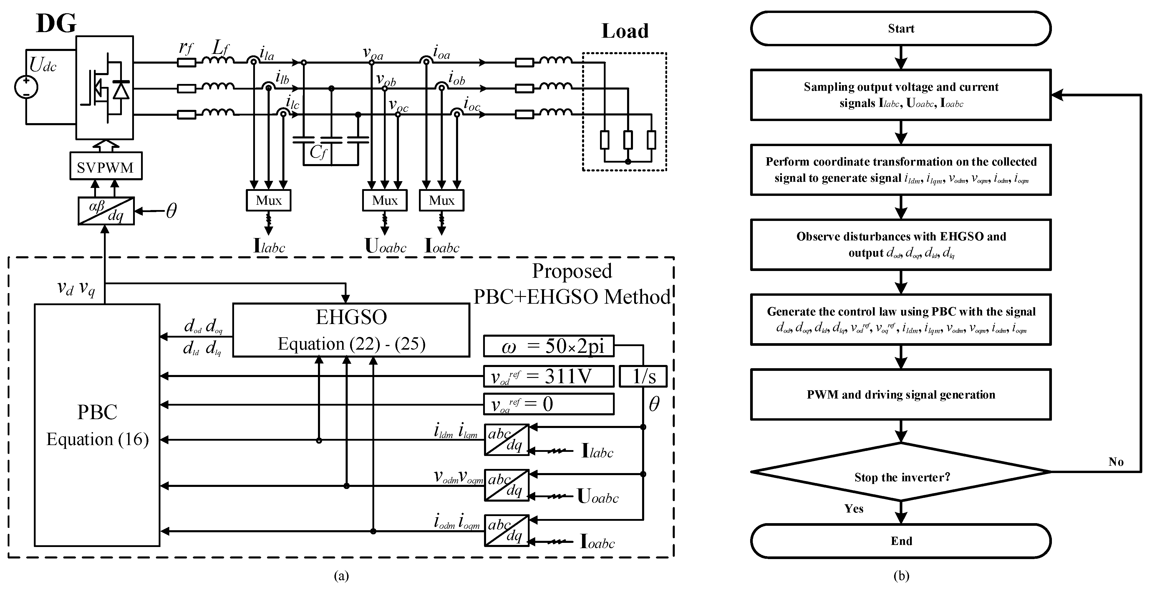
3. Design of the Proposed Disturbance-Rejection Passivity-Based Control

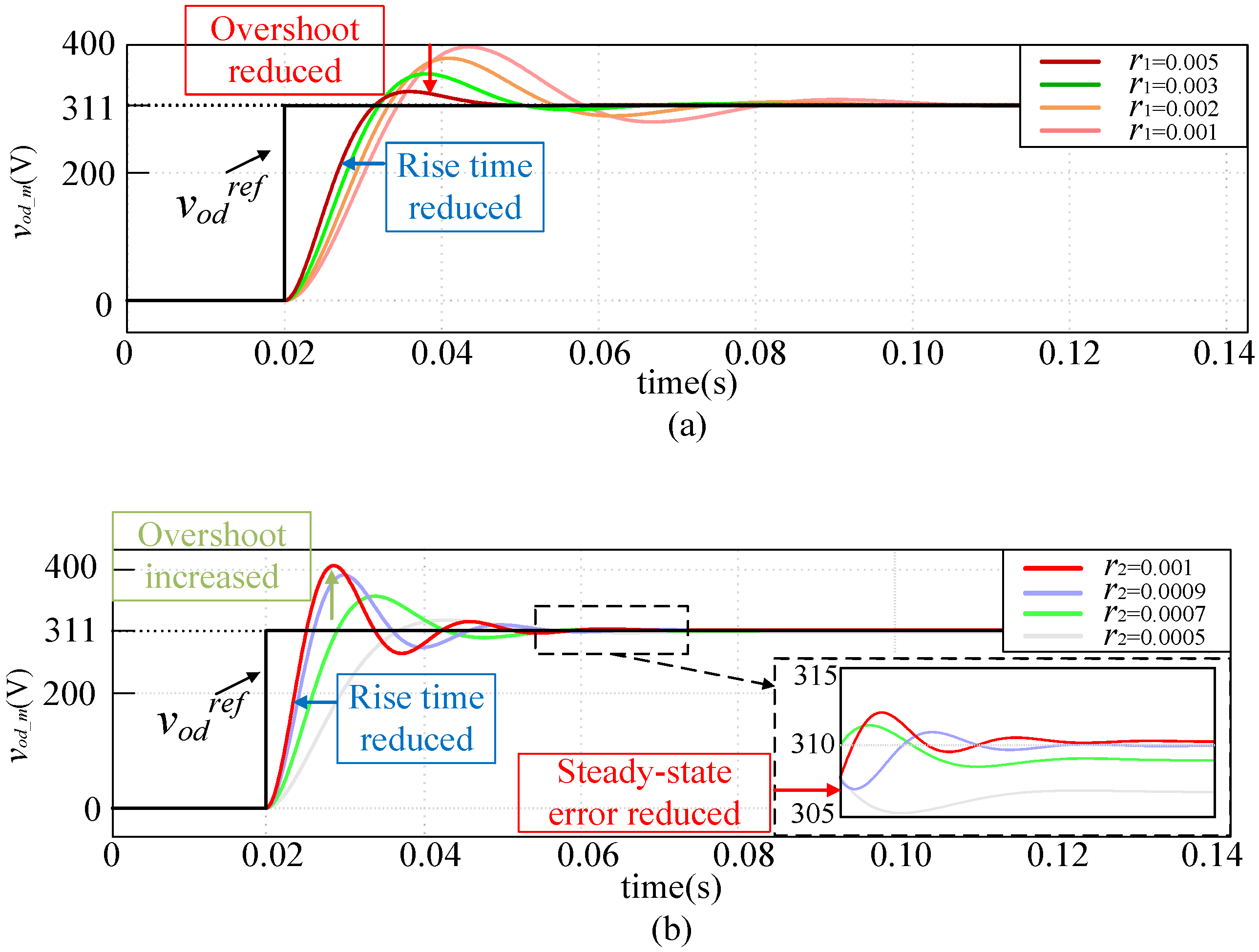
3.1. Design of the Proposed Passivity-Based Control

Defining the inverter’s state variables as x = (i_ldm i_lqm v_odm v_oqm)^T, Equation (3) can be derived into the standard Euler–Lagrange (EL) model as

$$M\dot{x}+Jx+Rx=u+\epsilon$$

(4)

where

$$\begin{array}{l}M=\left[\begin{array}{cccc}{L}_{fs}& 0& 0& 0\\ 0& L_{fs}& 0& 0\\ 0& 0& C_{fs}& 0\\ 0& 0& 0& C_{fs}\end{array}\right],J=\left[\begin{array}{cccc}0& -\omega L_{fs}& 1& 0\\ \omega L_{fs}& 0& 0& 1\\ -1& 0& 0& -\omega C_{fs}\\ 0& -1& \omega C_{fs}& 0\end{array}\right],\\ R=\left[\begin{array}{cccc}{r}_{fs}& 0& 0& 0\\ 0& r_{fs}& 0& 0\\ 0& 0& 0& 0\\ 0& 0& 0& 0\end{array}\right],u=\left[\begin{array}{c}{v}_d\\ v_q\\ 0\\ 0\end{array}\right],\epsilon =\left[\begin{array}{l}{L}_{fs}{d}_{ldm}\\ L_{fs}{d}_{lqm}\\ -i_{odm}+C_{fs}{d}_{od}\\ -i_{oqm}+C_{fs}{d}_{oq}\end{array}\right]\end{array}$$

(5)

where M is a positive definite matrix, representing the storage of energy; J is a skew-symmetric matrix, which represents the interconnection relationship; R is a symmetric positive definite matrix, representing energy dissipation; u is the control input; and ε stands for external disturbances.

To design the PBC controller, the inverter model’s passivity in the dq reference frame must first be verified. Since disturbances do not affect the system’s energy storage, they can be ignored during passivity analysis.

Based on Equation (2), we have

$${\displaystyle \frac{d}{dt}}\left[\underset{H_L}{\underbrace{\left(L_f{i}_{ld}^2+L_f{i}_{lq}^2\right)}}+\underset{H_C}{\underbrace{\left(C_f{v}_{od}^2+C_f{v}_{oq}^2\right)}}\right]=\left(v_d{i}_{ld}+v_q{i}_{lq}\right)-\left(r_f{i}_{ld}^2+r_f{i}_{lq}^2+v_{od}{i}_{od}+v_{oq}{i}_{oq}\right)$$

(6)

where H_L and H_C are the energy stored in the inductor and capacitor, respectively. The total energy storage of the inverter is H = H_L + H_C.

Integrating both sides of Equation (6), it yields

$$\underset{\mathbf{Energy}\mathbf{at}T\mathbf{moment}}{\underbrace{\mathit{H}(T)}}=\underset{\mathbf{Initial}\mathbf{energy}}{\underbrace{\mathit{H}(0)}}+\underset{\mathbf{Supplied}\mathbf{energy}}{\underbrace{{\displaystyle {\int }_0^T{\mathit{u}}^T(\tau )\mathit{i}(\tau )}d\tau }}-\underset{\mathbf{Dissipated}\mathbf{energy}}{\underbrace{{\displaystyle {\int }_0^T\left(r_f{i}_{ld}^2(\tau )+r_f{i}_{lq}^2(\tau )+{\mathit{u}}_o^T(\tau ){\mathit{i}}_o(\tau )\right)}d\tau }}$$

(7)

where u = [v_d v_q]^T, i = [i_ld i_lq]^T, i = [i_ld i_lq]^T, i_o = [i_od i_oq]^T.

The total energy storage of the inverter is denoted as H = x^T·M·x/2. Hence, combined with Equation (4), we have

$$\stackrel{·}{\mathit{H}}={\mathit{x}}^T\mathit{M}\stackrel{·}{\mathit{x}}={\mathit{x}}^T(\mathit{u}-\mathit{J}\mathit{x}-\mathit{R}\mathit{x})={\mathit{x}}^T\mathit{u}-{\mathit{x}}^T\mathit{R}\mathit{x}$$

(8)

According to the definition of passivity in [23], let y = x, Q(x) = x^T·R·x; it is known that the inverter’s model in the dq reference frame is strictly passive. Therefore, the design of passivity-based control is feasible.

Define the reference state variable as

$${\mathit{x}}^{*}={(\begin{array}{cccc}{i}_{ld}^{*}& i_{lq}^{*}& v_{od}^{*}& v_{oq}^{*}\end{array})}^T$$

(9)

And the state error vector as x_e = x − x*. Based on Equation (4), it is obtained that

$$\mathit{M}({\dot{\mathit{x}}}^{*}+{\dot{\mathit{x}}}_e)+\mathit{J}({\mathit{x}}^{*}+{\mathit{x}}_e)+\mathit{R}({\mathit{x}}^{*}+{\mathit{x}}_e)=\mathit{u}+\mathit{\epsilon }$$

(10)

Equation (10) can also be expressed as

$$\mathit{M}{\dot{\mathit{x}}}_e+\mathit{J}{\mathit{x}}_e+\mathit{R}{\mathit{x}}_e=\mathit{u}+\mathit{\epsilon }-\mathit{M}{\dot{\mathit{x}}}^{*}-\mathit{J}{\mathit{x}}^{*}-\mathit{R}{\mathit{x}}^{*}$$

(11)

To stabilize the inverter while operating, dampings are injected into the system. Define the damping matrix R_d as

$${\mathit{R}}_d=diag(\begin{array}{cccc}{r}_1& r_1& r_2& r_2\end{array})$$

(12)

The new impedance matrix R_new is then obtained after adding the damping matrix to the original system impedance, which is

$${\mathit{R}}_{new}=\mathit{R}+{\mathit{R}}_d$$

(13)

Based on the above analysis, the system model becomes

$$\mathit{M}{\dot{\mathit{x}}}_e+\mathit{J}{\mathit{x}}_e+{\mathit{R}}_{new}{\mathit{x}}_e=\mathit{u}+\mathit{\epsilon }-\mathit{M}{\dot{\mathit{x}}}^{*}-\mathit{J}{\mathit{x}}^{*}-\mathit{R}{\mathit{x}}^{*}+{\mathit{R}}_d{\mathit{x}}_e$$

(14)

Thus, the proposed passivity-based controller can be designed as

$$\mathit{u}=-\mathit{\epsilon }+\mathit{M}{\dot{\mathit{x}}}^{*}+\mathit{J}{\mathit{x}}^{*}+\mathit{R}{\mathit{x}}^{*}-{\mathit{R}}_d{\mathit{x}}_e$$

(15)

The control law in the dq reference frame reads

$$\left\{\begin{array}{l}{v}_d=-L_{fs}{d}_{ld}+L_{fs}{\dot{i}}_{ld}^{*}-\omega L_{fs}{i}_{lq}^{*}+v_{od}^{*}+r_{fs}{i}_{ld}^{*}-r_1(i_{ldm}-i_{ld}^{*})\\ v_q=-L_{fs}{d}_{lq}+L_{fs}{\dot{i}}_{lq}^{*}+\omega L_{fs}{i}_{ld}^{*}+v_{oq}^{*}+r_{fs}{i}_{lq}^{*}-r_1(i_{lqm}-i_{lq}^{*})\\ i_{ld}^{*}=i_{odm}-C_{fs}{d}_{od}+C_{fs}{\dot{v}}_{od}^{*}-\omega C_{fs}{v}_{oq}^{*}-r_2(v_{odm}-v_{od}^{*})\\ i_{lq}^{*}=i_{oqm}-C_{fs}{d}_{oq}+C_{fs}{\dot{v}}_{oq}^{*}+\omega C_{fs}{v}_{od}^{*}-r_2(v_{oqm}-v_{oq}^{*})\end{array}\right.$$

(16)

For the inverter, considering the Lyapunov function as

$$V(e)={\displaystyle \frac{1}{2}}{e}^{\mathbf{T}}Me$$

(17)

where M > 0 (M is a positive definite matrix), V(e) > 0, and ∀e ≠ 0.

Combining with (5), M is symmetric while J is antisymmetric. Hence, the derivative of the Lyapunov function is

$$\dot{V}(e)=e^{\mathbf{T}}M\dot{e}=e^{\mathbf{T}}\left(\mathsf{\psi }-Je-Re\right)=-e^{\mathbf{T}}Re<0$$

(18)

According to Lyapunov stability theory, the closed-loop system is asymptotically stable. In addition, when ||e|| → ∞, V → ∞, the closed-loop system is globally asymptotically stable.

Hence, it is known that the proposed PBC control can stabilize the inverter under all operating conditions.

Currently, a systematic parameter tuning method for PBC is still lacking to ensure the inverter’s dynamic performance. To address that, a parameter optimization and tuning method is provided here, which is simply achieved in combination with simulation analysis. For better understanding, the parameter tuning process is exemplified using the state variable x₁ within the EHGSO framework.

Figure 2 presents the dynamic response of the inverter’s output voltage under different parameters of the PBC controller. In the test, the reference value of the output voltage in the d-axis is set to 311 V, and a resistive load of R_L = 10 Ω is connected to the output. Disturbances are ignored during the testing process. As illustrated in Figure 2a, an increase in the virtual damping resistor r₁ results in a faster dynamic response and a reduction in overshoot. Moreover, Figure 2b shows that an increase in r₁ and r₂ leads to a faster dynamic response and a decrease in steady-state error, albeit with a slight increase in overshoot. Thus, by appropriately adjusting the virtual damping resistors r₁ and r₂, a trade-off between dynamic performance and steady-state error can be achieved. Following the above process, r₁ and r₂ are finally selected as 0.005 and 0.001, respectively.

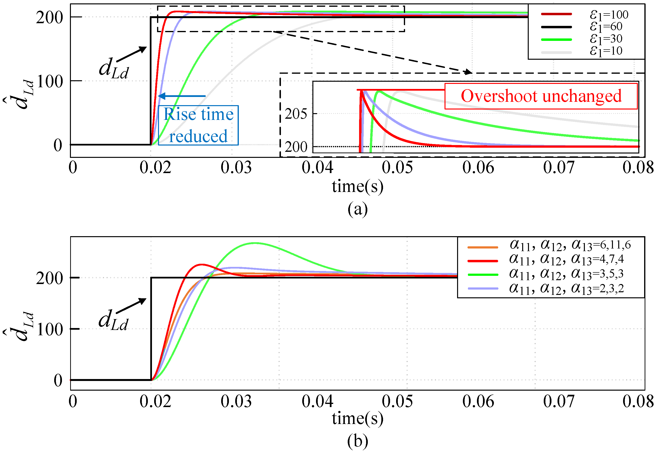
3.2. Design of the Extended High-Gain State Observer

It is known from Equation (16) that the system model depends on the exact values of the disturbance quantities d_ld, d_lq, d_od, and d_oq. However, in real applications, these disturbances are usually unmeasurable and unknown. To solve this problem, the extended high-gain state observer (EHGSO) is adopted in this section to observe the disturbances d_ld, d_lq, d_od, and d_oq to compensate for their impact on the system, thereby improving the control accuracy and robustness of the system [24].

To simplify the analysis, the design for the state variable i_{Ld_m} and its corresponding disturbance d_Ld is taken as an example. The derivation process for the other state variables i_{Lq_m}, v_{od_m}, and v_{oq_m} and disturbances d_Lq, d_Cd, and d_Cq is identical and thus will not be reiterated. Only the final results are presented.

Define observation error (η) as

$$\mathsf{\eta }={[{\eta }_1,{\eta }_2,{\eta }_3]}^{\mathrm{T}}={[i_{Ld\_m}-{\widehat{i}}_{Ld\_m},(d_{Ld}-{\widehat{d}}_{Ld})/{\epsilon }_1,({\dot{d}}_{Ld}-{\widehat{\dot{d}}}_{Ld})/{\epsilon }_1^2]}^{\mathrm{T}}$$

(19)

The error equation of EHGSO can be expressed as

$$\dot{\mathit{\eta }}={\epsilon }_1\mathit{A}\mathit{\eta }+\mathit{B}{\ddot{d}}_1$$

(20)

where $\mathbf{A}=\left[\begin{array}{ccc}-{\alpha }_{11}& 1& 0\\ -{\alpha }_{12}& 0& 1\\ -{\alpha }_{13}& 0& 0\end{array}\right]$, $\mathit{B}=\left[\begin{array}{c}0\\ 0\\ 1/{\epsilon }_1^2\end{array}\right]$, and α₁₁~α₁₃ are parameters ensuring that A is a Hurwitz matrix.

Substituting Equation (19) into Equation (20) yields

$$\left\{\begin{array}{l}{\dot{i}}_{ldm}-{\dot{\widehat{i}}}_{ldm}=-{\epsilon }_1{\alpha }_{11}(i_{ldm}-{\widehat{i}}_{ldm})+d_{ld}-{\widehat{d}}_{ld}\\ {\dot{\widehat{d}}}_{ld}={\epsilon }_1^2{\alpha }_{12}(i_{ldm}-{\widehat{i}}_{ldm})+{\widehat{\dot{d}}}_{ld}\\ {\dot{\widehat{\dot{d}}}}_{ld}={\epsilon }_1^3{\alpha }_{13}(i_{ldm}-{\widehat{i}}_{ldm})\end{array}\right.$$

(21)

Combining with Equation (16), we obtain

$$\left\{\begin{array}{l}{\dot{\widehat{i}}}_{ld}=-r_f{i}_{ldm}/L_{fs}+\omega i_{lqm}+(v_d-v_{odm})/L_{fs}+{\epsilon }_1{\alpha }_{11}(i_{ldm}-{\widehat{i}}_{ld})+{\widehat{d}}_{ld}\\ {\dot{\widehat{d}}}_{ld}={\epsilon }_1^2{\alpha }_{12}(i_{ldm}-{\widehat{i}}_{ld})+{\widehat{\dot{d}}}_{ld}\\ {\dot{\widehat{\dot{d}}}}_{ld}={\alpha }_{13}{\epsilon }_1^3(i_{ldm}-{\widehat{i}}_{ld})\end{array}\right.$$

(22)

Similarly, the EHGSO corresponding to the other three state variables are as follows.

$$\left\{\begin{array}{l}{\dot{\widehat{i}}}_{lq}=-r_f{i}_{lqm}/L_{fs}-\omega i_{ldm}+(v_q-v_{oqm})/L_{fs}+{\epsilon }_2{\alpha }_{21}(i_{lqm}-{\widehat{i}}_{lq})+{\widehat{d}}_{lq}\\ {\dot{\widehat{d}}}_{lq}={\epsilon }_2^2{\alpha }_{22}(i_{lqm}-{\widehat{i}}_{lq})+{\widehat{\dot{d}}}_{lq}\\ {\dot{\widehat{\dot{d}}}}_{lq}={\alpha }_{23}{\epsilon }_2^3(i_{lqm}-{\widehat{i}}_{lq})\end{array}\right.$$

(23)

$$\left\{\begin{array}{l}{\dot{\widehat{v}}}_{od}=\omega v_{oqm}+(i_{ldm}-i_{odm})/C_{fs}+{\epsilon }_3{\alpha }_{31}(v_{odm}-{\widehat{v}}_{od})+{\widehat{d}}_{od}\\ {\dot{\widehat{d}}}_{od}={\epsilon }_{\mathbf{3}}^{\mathbf{2}}{\alpha }_{32}(v_{odm}-{\widehat{v}}_{od})+{\widehat{\dot{d}}}_{od}\\ {\dot{\widehat{\dot{d}}}}_{od}={\alpha }_{33}{\epsilon }_3^3(v_{odm}-{\widehat{v}}_{od})\end{array}\right.$$

(24)

$$\left\{\begin{array}{l}{\dot{\widehat{v}}}_{oq}=-\omega v_{odm}+(i_{lqm}-i_{oqm})/C_{fs}+{\epsilon }_4{\alpha }_{41}(v_{oqm}-{\widehat{v}}_{oq})+{\widehat{d}}_{oq}\\ {\dot{\widehat{d}}}_{oq}={\epsilon }_{\mathbf{4}}^{\mathbf{2}}{\alpha }_{42}(v_{oqm}-{\widehat{v}}_{oq})+{\widehat{\dot{d}}}_{oq}\\ {\dot{\widehat{\dot{d}}}}_{oq}={\alpha }_{43}{\epsilon }_4^3(v_{oqm}-{\widehat{v}}_{oq})\end{array}\right.$$

(25)

where superscript ^ denotes the estimates of the corresponding variables; ε₁, ε₂, ε_3, and ε₄ are the observers’ scaling gains, which are greater than 1. α₁₁–α₁₃, α₂₁–α₂₃, α₃₁–α_33, and α₄₁–α₄₃ are observers’ coefficients, which are the coefficients of Hurwitz polynomials h₁(s) = s³ + α₁₁s² + α₁₂s + α₁₃, h₂(s) = s³ + α₂₁s² + α₂₂s + α₂₃, h₃(s) = s³ + α₃₁s² + α₃₂s + α_33, and h₄(s) = s³ + α₄₁s² + α₄₂s + α₄₃, respectively.

Next, a stability analysis of the EHGSO is conducted. For simplicity, the stability analysis of the EHGSO given in Equation (22) is given as an example here. Similar analyses can be applied to other EHGSOs.

Assuming that the disturbance d_ld is second-order continuously differentiable and the derivative is bounded (most disturbances of inverters satisfy such assumption), that is

$$\max \left\{\sup \left|{\dot{d}}_{ld}\right|,\sup \left|{\ddot{d}}_{ld}\right|\right\}\le D_{ld}$$

(26)

where D_ld is a positive number.

Since α₁₁–α₁₃ are the coefficients of Hurwitz polynomial h₁(s), the system matrix A is the Hurwitz matrix. Therefore, according to the Lyapunov stability theory, there must be a positive definite symmetric matrix P satisfying A^TP + PA = −I. Choose the candidate Lyapunov function as

$$W_e={\mathit{\eta }}^{\mathrm{T}}\mathit{P}\mathit{\eta }$$

(27)

The derivative of the Lyapunov function is

$$\begin{array}{cc}\hfill {\dot{W}}_e& ={\mathit{\eta }}^{\mathrm{T}}\mathit{P}\dot{\mathit{\eta }}+{\dot{\mathit{\eta }}}^{\mathrm{T}}\mathit{P}\mathit{\eta }\hfill \\ \hfill & ={\epsilon }_1{\mathit{\eta }}^{\mathrm{T}}(\mathit{P}\mathit{A}+{\mathit{A}}^{\mathrm{T}}\mathit{P})\mathit{\eta }+({\mathit{\eta }}^{\mathrm{T}}\mathit{P}\mathit{B}+{\mathit{B}}^{\mathrm{T}}P\mathit{\eta }){\ddot{d}}_1\hfill \\ \hfill & =-{\epsilon }_1{‖\mathit{\eta }‖}^2+2{\mathit{\eta }}^{\mathrm{T}}\mathit{P}\mathit{B}{\ddot{d}}_1\hfill \\ \hfill & \le -{\epsilon }_1{‖\mathit{\eta }‖}^2+2{\phi }_1‖\mathit{\eta }‖\hfill \\ \hfill & \le -({\epsilon }_1-1){‖\mathit{\eta }‖}^2+{\phi }_1^2\hfill \end{array}$$

(28)

where ${\phi }_1=D_1\cdot \sqrt{{\lambda }_1}/{\epsilon }_1^2$. λ₁ is the maximum eigenvalue of the matrix P^TP.

According to Equation (27), we have

$${‖\mathit{\eta }‖}^2\ge W_e/\sqrt{{\lambda }_1}>0$$

(29)

Substituting Equation (29) into Equation (28) yields

$${\dot{W}}_e\le -({\epsilon }_1-1){‖\mathit{\eta }‖}^2+{\phi }_1^2\le -({\epsilon }_1-1)W_e/\sqrt{{\lambda }_1}+{\phi }_1^2$$

(30)

Let $\mathsf{\Omega }:=\left\{\mathsf{\eta }\in {ℝ}^3|W_e\le {\delta }_1\right\}$, where δ₁ is a positive constant that is arbitrarily small, for any $\mathsf{\eta }\notin \mathsf{\Omega }$, $W_e>{\delta }_1$ always holds.

For any given constant δ₁, select ε₁ large enough to satisfy

$${\displaystyle \frac{2D_1^2{\lambda }_1\sqrt{{\lambda }_1}}{{\epsilon }_1^4({\epsilon }_1-1)}}\le {\delta }_1$$

(31)

Equation (31) can be also expressed as

$${\phi }_1^2={\displaystyle \frac{D_1^2{\lambda }_1}{{\epsilon }_1^4}}\le 0.5({\epsilon }_1-1){\delta }_1/\sqrt{{\lambda }_1}$$

(32)

Therefore, when W_e > δ₁, we have

$$\begin{array}{cc}\hfill {\dot{W}}_e& \le -({\epsilon }_1-1)W_e/\sqrt{{\lambda }_1}+{\phi }_1^2\hfill \\ \hfill & \le -({\epsilon }_1-1){\delta }_1/\sqrt{{\lambda }_1}+{\phi }_1^2\hfill \\ \hfill & \le -({\epsilon }_1-1){\delta }_1/\sqrt{{\lambda }_1}+0.5({\epsilon }_1-1){\delta }_1/\sqrt{{\lambda }_1}\hfill \\ \hfill & =-0.5({\epsilon }_1-1){\delta }_1/\sqrt{{\lambda }_1}\hfill \\ \hfill & <0\hfill \end{array}$$

(33)

According to Equation (32), when W_e > δ₁, the derivative of the Lyapunov function can be less than zero by selecting a sufficiently large ε₁, so the observation error (η) will converge to Ω. In addition, it can be observed from Equation (31) that ε₁ is approximately negatively correlated with δ₁. When λ_1, and D₁ remain unchanged, δ₁ will decrease with the increase of ε₁. Therefore, by amplifying ε₁, δ₁ can be almost equal to zero, which means that Ω can be infinitesimal, so the observation error (η) can be adjusted as small as possible and thus negligible.

Following the above procedures, the effectiveness of the EHGSOs for disturbances d_lq, d_od, and d_oq can also be proved.

As the observer’s performance is closely related to its parameters, we proceed with the design of the observer parameters. Keeping in mind that to effectively suppress the impact of complex disturbances, the EHGSO’s dynamic response should be faster than that of the PBC controller. Following the aforementioned adjustment process for the PBC parameters, the dynamic response of the EHGSO under different control parameters can be obtained.

As shown in Figure 3, a disturbance (d_Ld) with an amplitude of 200 is applied to the system. From Figure 3a, it is seen that the larger the observer gain (ε₁), the faster the dynamic response. Considering the requirement for the dynamic response, ε₁ = 100 is finally selected. Furthermore, Figure 3b shows that with a constant observer gain (ε₁), variations in α₁₁ to α₁₃ cause changes in the overshoot and settling time. Considering both dynamic response and overshoot requirements, α₁₁ = 6, α₁₂ = 11, and α₁₃ = 6 are ultimately chosen. Compared with Figure 2, it can be observed that the response time of EHGSO is shorter than that of PBC, which is consistent with the desired dynamic performance.

Figure 4 shows the block diagram and a control flowchart of the proposed disturbance-rejection passivity-based control for the inverter. Since this paper’s research object is a standalone photovoltaic/wind turbine inverter, the voltage and frequency reference values are given directly.

4. Experiments

Figure 5 shows an experimental platform for a 15 kVA inverter built in the lab. The controller is achieved using DSP (TMS320F28335) and FPGA (LCMXO2-4000HC). The parameters of the inverter and the controller are listed in

Table 2. Parameters of system.

Symbol	Value
Nominal DC voltage Udc/V	700
Switching frequency F/kHz	15
The power rating of the inverter Pp/kW	15
Phase voltage Unrms/V	220
Filter inductor Lf/mH	1.5
Equivalent series resistance of filter inductor rf/mΩ	80
Filter capacitor Cf/µF	15

and

Table 3. Parameters of the improved PBC controller.

Symbol	Value
Virtual damping resistor r1	0.005
Virtual damping resistor r2	0.001
Coefficients of observer α11, α21, α31, α41	6
Coefficients of observer α12, α22, α32, α42	11
Coefficients of observer α13, α23, α33, α43	6
Observer scaling gains e1, e2	100
Observer scaling gains e3, e4	10

, respectively.

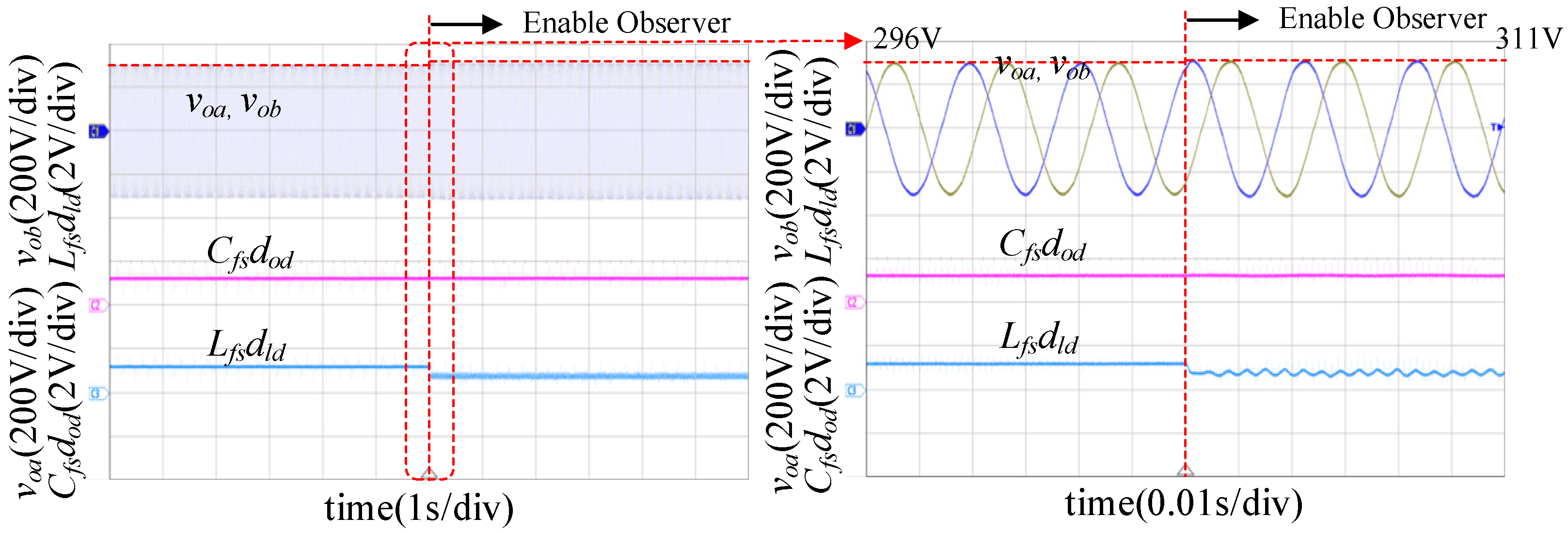
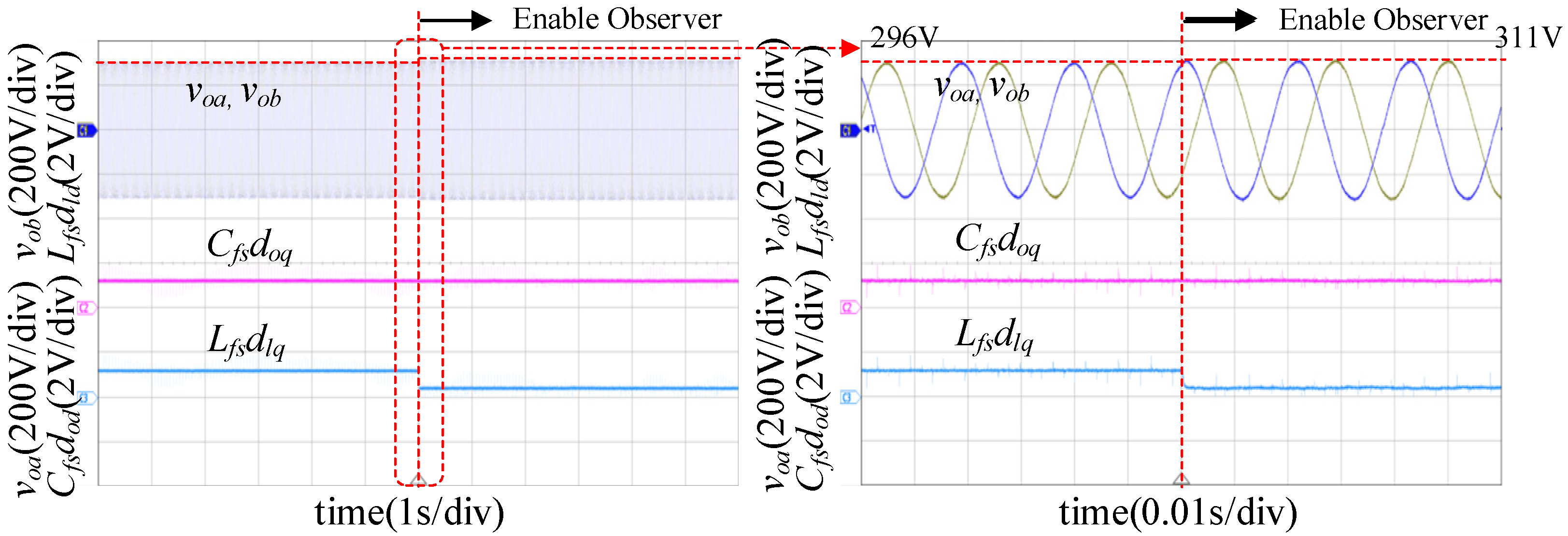
4.1. Experimental Results of the Inverter with and without the Observer

Figure 6 and Figure 7 present the experimental results for the inverter controlled by the proposed controller, both with and without the EHGSO. The inverter’s output voltage, when controlled solely by the PBC, exhibits a steady-state error of approximately 15 V. This discrepancy can be attributed to model errors, parameter uncertainties, and other perturbations inherent in the system. However, upon activation of the EHGSO, this steady-state error is effectively eliminated. The EHGSO’s capability to observe and compensate for disturbances enables the PBC controller to counteract these influences, thereby achieving a more accurate and stable output voltage. This demonstrates the efficacy of integrating EHGSO with PBC in mitigating the impact of various disturbances and enhancing the overall performance of the inverter control system.

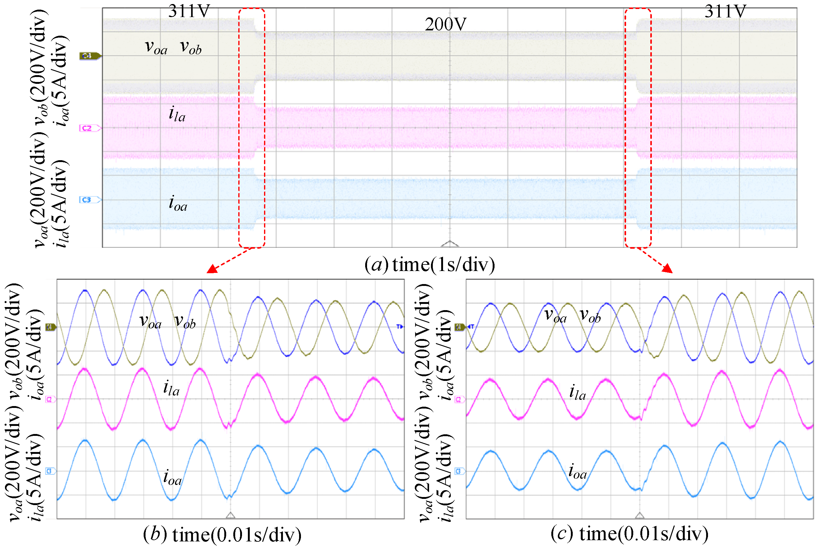
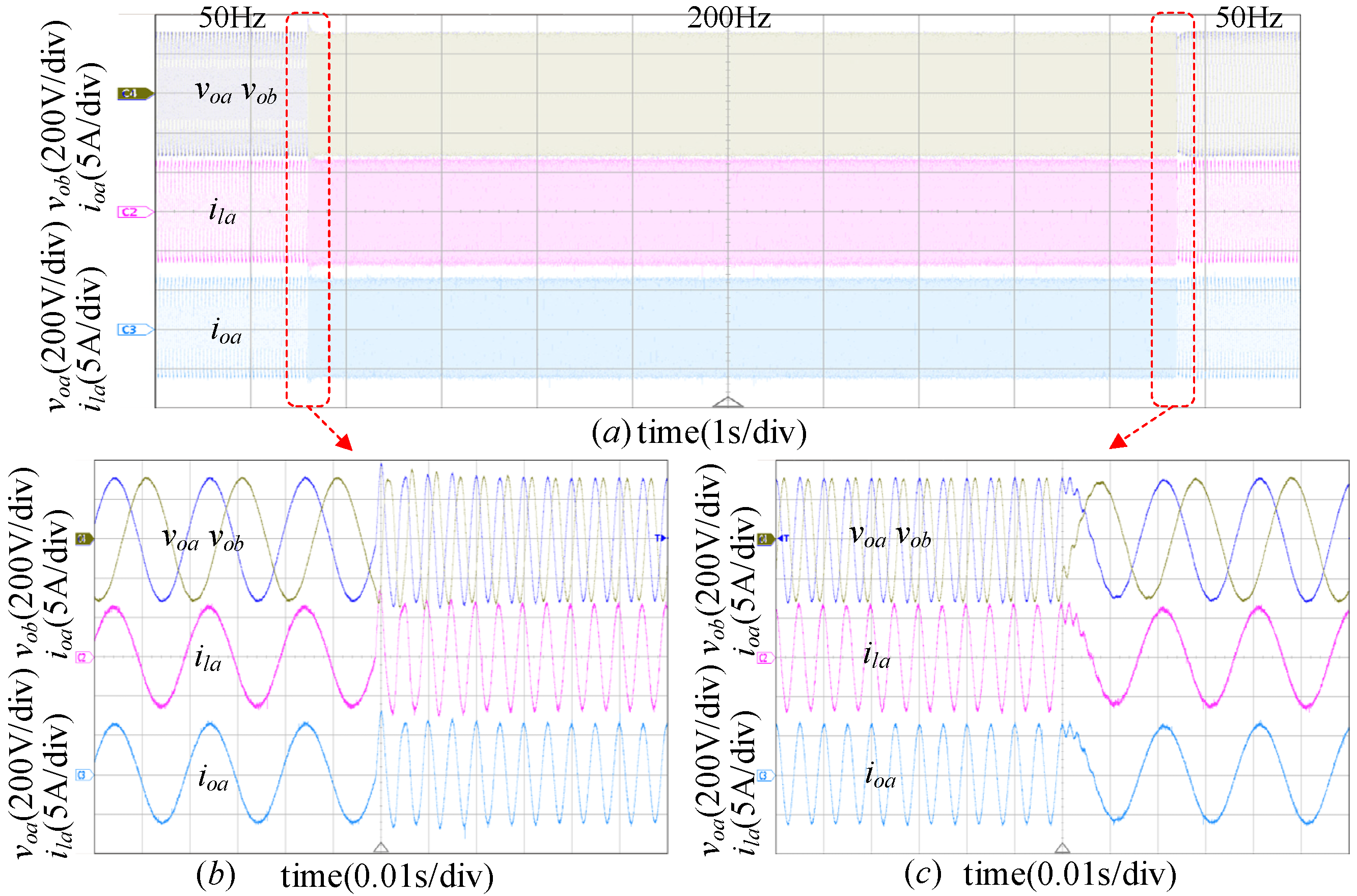
4.2. Voltage and Frequency Adjusting Performances

Figure 8 and Figure 9 show the experimental results of adjusting the output voltage and frequency of the inverter controlled by improved PBC, respectively. The inverter with the proposed PBC controller responds fast when the output voltage reference is adjusted from 311 V to 200 V, as shown in Figure 8b. Low distortions are observed in this transient. This is also the case when the voltage reference is increased from 200 V to 311 V, as shown in Figure 8c. This result indicates that the inverter with the proposed PBC has a good output voltage adjustment performance.

In Figure 9, the frequency reference is changed from 50 Hz to 200 Hz and then back to 50 Hz. The results shown in Figure 9b,c, which are zoomed-in results during transients, show that with the proposed PBC, the inverter can perform fast dynamic frequency regulation.

As a result, the proposed controller can achieve zero and fast-tracking for the inverter’s frequency under varying frequency references.

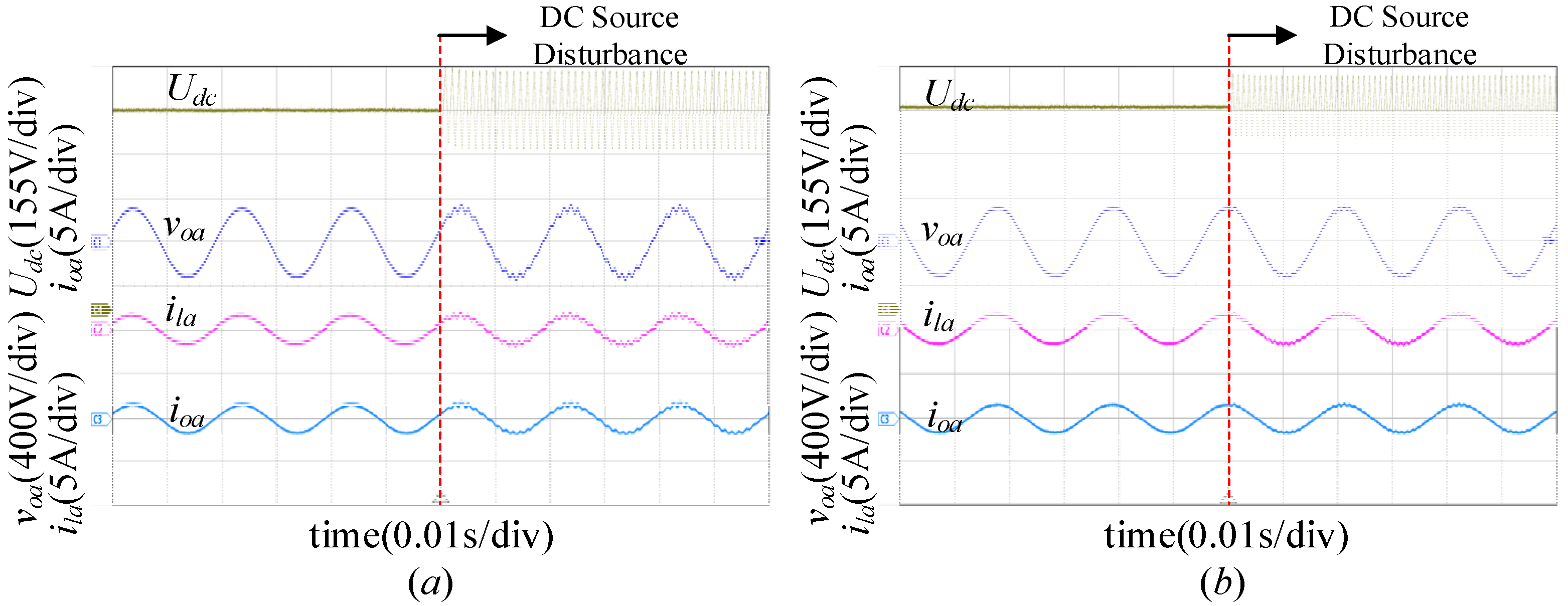
4.3. Comparisons of the Inverter’s Performances with Proposed PBC and PI Controllers

To demonstrate the effectiveness of the proposed PBC method, its performances are compared with the widely used traditional PI controller. The PI controller’s parameters were tuned according to the guidelines provided in reference [25] to achieve good performance. The specific parameters of the PI controller are listed in

Table 4. Parameters of the PI controller.

Symbol	Value
Proportional gain of current loop PI controller kpi	15
Integral gain of current loop PI controller kii	400
Proportional gain of voltage loop PI controller kpv	0.045
Integral gain of voltage loop PI controller kiv	45

.

As shown in Figure 10, when the inverter is under constant power loads (10 kW active power and 2 kVar reactive power), it starts to oscillate with the PI controller, leading to instability problems. However, the improved PBC can stabilize the inverter, maintaining stable output voltage and current waveform.

Furthermore, when the filter inductance (L_f) varies from 1.5 mH to 1 mH (the filter parameter reduces up to 33%), which is a severe condition for the inverter’s operation, the traditional PI controller has high-frequency oscillation as it can not bear such strong parameter variation, as shown in Figure 11a. However, the output voltage and current of the inverter with the proposed PBC do not change so much, as shown in Figure 11b. This is because the proposed PBC is not sensitive to parameter changes, which is consistent with the theoretical analysis.

In addition, as shown in Figure 12, when the filter capacitance (C_f) reduces from 25 µF to 1 µF (the filter parameter reduces up to 96%), the output voltage and current waveforms of the inverter with PBC are better than those of the inverter with PI controller. Again, it is proved that the proposed PBC is not sensitive to the system parameter changes.

Finally, as shown in Figure 13, when the DC input voltage has a disturbance of about ±155 V (the input voltage approximately varies 22%), the proposed PBC can better suppress the source-side disturbance than the traditional PI controller. Higher-quality voltage and current waveforms are obtained.

5. Conclusions

To improve the stability of the standalone inverter under numerous influencing factors such as time-varying parameter uncertainties, modeling errors, and external random disturbances, this paper proposes a composite controller that integrates EHGSO and PBC. Firstly, an extended state model of the system is established under the influence of parameter uncertainties, modeling errors, and external random disturbances. Based on this model, a PBC controller that can ensure the global system stability of the inverter is derived. Concurrently, a method utilizing EHGSO for online observation and compensation of various disturbances within the system is proposed, ensuring system robustness and disturbance rejection performance. Experimental results performed by a 15 kVA inverter prototype show that the proposed control is able to ensure the inverter’s stable operation under the following conditions: (a) constant power load; (b) the filter inductance and capacitance reduce up to 33% and 96%; and (c) the input voltage varies more than 22%. Therefore, with the proposed controller, good static and dynamic performances, as well as high robustness, are achieved for the inverters.

Despite the promising results, the proposed method cannot be used under unbalanced three-phase loads, potentially limiting its application in real applications. We acknowledge this limitation and plan to address it in future research.

References

1. Uddin, M.; Mo, H.; Dong, D.; Elsawah, S.; Zhu, J.; Guerrero, J.M. Microgrids: A review, outstanding issues and future trends. Energy Strategy Rev. 2023, 49, 101127. [Google Scholar] [CrossRef]
2. Hasheminasab, S.; Alzayed, M.; Chaoui, H. A Review of Control Techniques for Inverter-Based Distributed Energy Resources Applications. Energies 2024, 17, 2940. [Google Scholar] [CrossRef]
3. Zhang, Q.; Zhai, Z.; Mao, M.; Wang, S.; Sun, S.; Mei, D.; Hu, Q. Control and Intelligent Optimization of a Photovoltaic (PV) Inverter System: A Review. Energies 2024, 17, 1571. [Google Scholar] [CrossRef]
4. Hosseinzadeh, N.; Aziz, A.; Mahmud, A.; Gargoom, A.; Rabbani, M. Voltage stability of power systems with renewable-energy inverter-based generators: A review. Electronics 2021, 10, 115. [Google Scholar] [CrossRef]
5. Fazal, S.; Haque, M.E.; Arif, M.T.; Gargoom, A.; Oo, A.M.T. Grid integration impacts and control strategies for renewable based microgrid. Sustain. Energy Technol. Assess. 2023, 56, 103069. [Google Scholar] [CrossRef]
6. Pogaku, N.; Prodanovic, M.; Green, T.C. Modeling, analysis and testing of autonomous operation of an inverter-based microgrid. IEEE Trans. Power Electron. 2007, 22, 613–625. [Google Scholar] [CrossRef]
7. Li, Y.; Meng, K.; Dong, Z.Y.; Zhang, W. Sliding framework for inverter-based microgrid control. IEEE Trans. Power Syst. 2020, 35, 1657–1660. [Google Scholar] [CrossRef]
8. Leitner, S.; Yazdanian, M.; Mehrizi-Sani, A.; Muetze, A. Small-signal stability analysis of an inverter-based microgrid with internal model-based controllers. IEEE Trans. Smart Grid 2017, 9, 5393–5402. [Google Scholar] [CrossRef]
9. Peng, Y.; Shuai, Z.; Liu, X.; Li, Z.; Guerrero, J.M.; Shen, Z.J. Modeling and stability analysis of inverter-based microgrid under harmonic conditions. IEEE Trans. Smart Grid 2019, 11, 1330–1342. [Google Scholar] [CrossRef]
10. Xie, Z.; Chen, Y.; Wu, W.; Wang, Y.; Gong, W.; Guerrero, J.M. Frequency coupling admittance modeling of quasi-PR controlled inverter and its stability comparative analysis under the weak grid. IEEE Access 2021, 9, 94912–94922. [Google Scholar] [CrossRef]
11. Yadav, M.; Jaiswal, P.; Singh, N. Fuzzy Logic-Based Droop Controller for Parallel Inverter in Autonomous Microgrid Using Vectored Controlled Feed-Forward for Unequal Impedance. J. Inst. Eng. (India) Ser. B 2021, 102, 691–705. [Google Scholar] [CrossRef]
12. Habib, M.; Ladjici, A.A.; Harrag, A. Microgrid management using hybrid inverter fuzzy-based control. Neural Comput. Appl. 2020, 32, 9093–9111. [Google Scholar] [CrossRef]
13. Yang, Y.; Wai, R.J. Design of adaptive fuzzy-neural-network-imitating sliding-mode control for parallel-inverter system in islanded micro-grid. IEEE Access 2021, 9, 56376–56396. [Google Scholar] [CrossRef]
14. Li, Z.; Cheng, Z.; Li, S.; Si, J.; Gao, J.; Dong, W.; Das, H.S. Virtual synchronous generator and SMC-based cascaded control for voltage-source grid-supporting inverters. IEEE J. Emerg. Sel. Top. Power Electron. 2021, 10, 2722–2736. [Google Scholar] [CrossRef]
15. Heins, T.; Joševski, M.; Gurumurthy, S.K.; Monti, A. Centralized model predictive control for transient frequency control in islanded inverter-based microgrids. IEEE Trans. Power Syst. 2022, 38, 2641–2652. [Google Scholar] [CrossRef]
16. Liu, E.; Han, Y.; Zalhaf, A.S.; Yang, P.; Wang, C. Performance evaluation of isolated three-phase voltage source inverter with LC filter adopting different MPC methods under various types of load. Control Eng. Pract. 2023, 135, 105520. [Google Scholar] [CrossRef]
17. Zeng, J.; Huang, Z.; Huang, Y.; Qiu, G.; Li, Z.; Yang, L.; Yang, B.; Yu, T. Modified linear active disturbance rejection control for microgrid inverters: Design, analysis, and hardware implementation. Int. Trans. Electr. Energy Syst. 2019, 29, e12060. [Google Scholar] [CrossRef]
18. Shi, H.; Zhou, J.; Zhang, J.; Feng, K.; Su, G. A voltage recovered control strategy for microgrid inverters based on Narendra-MRAC. Meas. Control 2023, 56, 403–410. [Google Scholar] [CrossRef]
19. Zhao, E. Research on Multi-Scale Instability Mechanism and Robust Passivity Control Method for Isolated Microgrids. Ph.D. Thesis, University of Electronic Science and Technology of China, Chengdu, China, 2023. [Google Scholar]
20. Zhao, J.; Wu, W.; Gao, N.; Wang, H.; Chung, H.S.H.; Blaabjerg, F. Combining passivity-based control with active damping to improve stability of LCL filtered grid-connected voltage source inverte. In Proceedings of the 2018 IEEE International Power Electronics and Application Conference and Exposition (PEAC), Shenzhen, China, 4–7 November 2018. [Google Scholar]
21. Zonetti, D.; Bergna-Diaz, G.; Ortega, R.; Monshizadeh, N. PID passivity-based droop control of power converters: Large-signal stability, robustness and performance. Int. J. Robust Nonlinear Control 2022, 32, 1769–1795. [Google Scholar] [CrossRef]
22. Lai, J.; Yin, X.; Jiang, L.; Yin, X.; Wang, Z.; Ullah, Z. Disturbance-observer-based PBC for static synchronous compensator under system disturbances. IEEE Trans. Power Electron. 2019, 34, 11467–11481. [Google Scholar] [CrossRef]
23. Lee, T.S. Lagrangian modeling and passivity-based control of three-phase AC/DC voltage-source converters. IEEE Trans. Ind. Electron. 2004, 51, 892–902. [Google Scholar] [CrossRef]
24. Freidovich, L.B.; Khalil, H.K. Performance recovery of feed-back-linearization-based designs. IEEE Trans. Autom. Control 2008, 53, 2324–2334. [Google Scholar] [CrossRef]
25. Skogestad, S. Simple analytic rules for model reduction and PID controller tuning. J. Process Control 2003, 13, 291–309. [Google Scholar] [CrossRef]
Figure 1. Schematic diagram of a typical inverter.
Electronics 13 02851 g001
Figure 2. Dynamic response of inverter output voltage under different PBC control parameters: (a) r2 unchanged, r1 varies; (b) r1 unchanged, r2 varies.
Electronics 13 02851 g002
Figure 3. Dynamic response of EHGSO under different control parameters.: (a) α11~α13 unchanged, ε1 varies; (b) ε1 unchanged, α11~α13 varies.
Electronics 13 02851 g003
Figure 4. Block diagram of the inverter with PBC + EHGSO.
Electronics 13 02851 g004
Figure 5. Experimental platform.
Electronics 13 02851 g005
Figure 6. The experimental results of the inverter controlled by PBC with and without the EHGSO (disturbances in the d-axis).
Electronics 13 02851 g006
Figure 7. The experimental results of the inverter controlled by PBC with and without the EHGSO (disturbances in q-axis).
Electronics 13 02851 g007
Figure 8. The experimental results of adjusting the inverter’s output voltage with the proposed PBC.
Electronics 13 02851 g008
Figure 9. The experimental results of adjusting the inverter’s frequency with the proposed PBC.
Electronics 13 02851 g009
Figure 10. Experimental results of the inverter with CPLs: (a) with PI control and (b) with PBC.
Electronics 13 02851 g010
Figure 11. Experimental waveforms of the inverter with changing filter inductance: (a) with PI control and (b) with PBC.
Electronics 13 02851 g011
Figure 12. Experimental results of the inverter with changing capacitor value: (a) with PI control and(b) with PBC.
Electronics 13 02851 g012
Figure 13. Comparative experimental waveforms of the inverter with input disturbance: (a) with PI control and (b) with PBC.
Electronics 13 02851 g013