Short-Term Load Forecasting Method Based on Bidirectional Long Short-Term Memory Model with Stochastic Weight Averaging Algorithm

Abstract

To accommodate the rapid development of the distribution network of China, it is essential to research load forecasting methods with higher accuracy and stronger generalization capabilities in order to optimize distribution system control strategies, ensure the efficient and reliable operation of the power system, and provide a stable power supply to users. In this paper, a short-term load forecasting method is proposed for low-voltage distribution substations based on the bidirectional long short-term memory (BiLSTM) model. First, principal component analysis (PCA) and the fuzzy C-means method based on a genetic algorithm (GA-FCM) are used to extract the main influencing factors and classify different types of user electricity consumption behaviors. Then, the BiLSTM forecasting model utilizing the stochastic weight averaging (SWA) algorithm to enhance generalization capability is constructed. Finally, the load data from a low-voltage distribution substation in China over recent years are selected as a case study. Compared with conventional LSTM and BiLSTM prediction models, the annual electricity load curves for various user types forecasted by the PCA-BiLSTM model are more closely aligned with actual data curves. The proposed BiLSTM forecasting model exhibits higher accuracy and can forecast user electricity consumption data that more accurately reflect real-life usage.

1. Introduction

With the rapid development of the socio-economic landscape of China, the demand for electricity in society has sharply increased. As a direct-to-user link in the power system, the distribution network is vast and has a complex structure. The massive integration of new elements such as distributed renewable energy and electric vehicles at the medium and low voltage distribution network level, coupled with various uncertainties, has significantly changed the source and load characteristics of the power distribution system, bringing great challenges to the safe and efficient operation of the system [1,2]. There is an urgent need for more effective methods for analyzing and predicting the behavior characteristics of new types of distribution systems.

Load forecasting aims to predict the electricity demand by considering various factors such as regional and weather changes that affect the load on the distribution system. By analyzing historical load data, it seeks to uncover the inherent patterns of load changes and make prior estimates and predictions [3]. Accurate load forecasting is a prerequisite for optimizing the control strategy of the power distribution system, ensuring the safe and efficient operation of the system and a reliable power supply for users [4,5]. Load forecasting can be divided into system-level and distribution substation-level forecasting, in which the goal of system-level forecasting is to provide a basis for power departments at all levels to arrange dispatch plans, while the goal of distribution substation-level forecasting is to guide the arrangement of maintenance plans, realize advance warning, allocate emergency repair resources, and adjust operation modes and other distribution network work. From a system perspective, it covers many types of loads with complementary characteristics, making the overall regularity more significant. In contrast, the geographic scale of distribution substations is smaller, with a weaker overall load change regularity, making system-level forecasting methods inapplicable. In addition, for a long time, it has been difficult to achieve accurate load forecasting at the station level due to the measurement communication level, data conditions, and computing power of the distribution system. The application of advanced information technology such as edge computing improves the data collection and utilization capabilities of the edge side of the distribution system and enables the distribution network business to shift from the main station to the edge side [6,7]. This provides the basic conditions for more accurate substation load forecasting and proposes new methods for forecasting substation loads under the influence of multiple integrated factors. From the timescale analysis of load forecasting research, short-term load forecasting can help guide the daily production of the distribution network. At the same time, the characteristics of user electricity consumption are reflected by the daily load curve of users, which extracts valuable information from the daily load data of massive users, which helps to build accurate user portraits and ensure the effective implementation of demand-side response strategies. Therefore, accurate short-term and daily load forecasting results are of great significance for the normal operation of the power distribution system.

The research on electric load forecasting has achieved many results. Early studies mostly employed linear methods such as regression analysis [8,9], the time series method [10,11], improved algorithms based on gray theory [12,13], and the Kalman filter algorithm [14,15]. However, due to the complexity of load forecasting itself and the multitude of influencing factors, traditional linear methods often fail to effectively uncover the inherent characteristics of electricity load data, making accurate predictions difficult to achieve. With the gradual improvement in nonlinear theory and the popularization and application of artificial intelligence technology, a large number of application results based on traditional machine learning and its improved algorithms have emerged in the research of load forecasting and related technologies. Among them, Chapagain and Jiang [16,17] improved the traditional Bayesian forecasting model to improve the generalization ability of the model and obtain high forecasting accuracy, but when such methods face complex influencing factors, a problem of low prediction efficiency occurs due to a significant amount of calculation. Xi and Zhang [18,19] improved the accuracy of electricity load forecasting by improving the support vector machine regression (SVR) algorithm, which is more mature and can quickly obtain the global optimal solution, but it relies heavily on historical data, and the prediction effect becomes worse when the load significantly fluctuates.

Traditional machine learning and its improved algorithms have the following two problems in the application of load forecasting: relatively simple model structures that may not fully capture the information contained in the distribution system, and weaker capabilities in handling the time-series data problems. In recent years, deep learning has emerged as a machine learning algorithm that mimics the human brain’s mechanism to learn representations from data [20]. Deep learning models have significant complexity and strong non-linear mapping capabilities, enabling them to effectively explore data features and express the underlying patterns present in large-scale electricity data [21].

Sha et al. [22] proposed the use of a genetic algorithm to optimize the backpropagation (BP) neural network for load forecasting. Dong et al. [23] applied a limited Boltzmann machine with pre-trained weight values to improve load forecasting accuracy. These forward neural network-based methods exhibit high forecasting accuracy, but they suffer from drawbacks such as slow convergence, poor model interpretability, and susceptibility to overfitting. The recurrent neural network model represented by the long-short-term memory network (LSTM) adds a time-series information expression module on the basis of the serial of neurons to achieve the effective processing of the load data [24,25]. Electricity load changes are influenced by multiple factors with complex interconnections, making it challenging for a single model to comprehensively reflect these relationships. In order to solve the problem, ensemble forecasting methods have emerged. By leveraging the strengths of multiple models, the characteristics of load data can be fully explored and utilized, so that the model can be more expressive, to achieve the goal of improving the accuracy of load forecasting. Ding et al. [26] reduces the dimensionality of load-influencing factors through the stacking model and uses the LSTM network to achieve the rapid and accurate forecasting of short-term load. Wu et al. [27] proposed a short-term electricity load forecasting method based on a feature screening convolutional neural network–bidirectional long short-term memory network (CNN-BiLSTM) combination model, which improved the short-term prediction accuracy of multi-dimensional electricity load data.

Electric load values are influenced by various factors, and integrating datasets that represent these factors often results in a significant amount of redundant information. During model training, this can lead to overfitting, thereby reducing prediction accuracy. Furthermore, most of the current research has focused on the load characteristics alone, with modeling based purely on electrical characteristics without fully considering the differentiated electricity consumption behaviors of users, which inevitably leads to a decrease in prediction accuracy to some extent. In view of the above problems, this study focuses on the short-term and load forecasting in low-voltage substations, analyzes the factors influencing electricity consumption (including external factors and consumption behaviors), and constructs a BiLSTM model for daily substation load forecasting on an annual basis. The specific process involves the following steps: first, using principal component analysis (PCA) to calculate the correlations of various external factors and reducing dimensionality based on these correlations; second, extracting the electricity consumption behavior characteristics of substation users from daily load historical data and applying the fuzzy C-means method based on genetic algorithm (GA-FCM) algorithm for feature clustering of users; third, combining the dimensionality reduction results of external factors and using the BiLSTM model to predict daily load for users with different characteristics; and finally, aggregating proportionally to obtain the substation load forecasting model. Compared to general hybrid forecasting models and other machine learning methods, the approach in this paper divides influencing factors into external factors and electricity consumption behavior factors, enabling a more comprehensive exploration of load-influencing factor characteristics while ensuring prediction efficiency and improving accuracy. Additionally, in this paper, the effectiveness is validated of the proposed BiLSTM load forecasting method integrating multi-dimensional influencing factor analysis through simulation models based on data from a specific low-voltage substation of a power company.

2. Load Forecasting Methodology

2.1. PCA Algorithm

Electric load forecasting is a prediction problem of multi-index variables, where the increase in input characteristic variables will greatly increase the complexity of the problem and extend the computation time. PCA is used to explore the correlation between different influencing factors of electricity load, remove overlapping feature information, and reduce data dimension.

The basic idea of PCA is to describe the correlation relationship of the entire variable system with a small number of representative variables, which belongs to the multivariate statistical analysis method [28]. This method is based on linear transformation, which transforms the original variable into a new variable that is not related to the other while containing as much information as possible about the original variable. That is, by solving the orthogonal matrix of the original variable, the following conditions are met, that the sum of squares of the coefficients of each original variable is 1, and the covariance between each new variable is 0. In addition, the variance in the variables is used to reflect the amount of information contained during the analysis, and the variables are evaluated by calculating the cumulative contribution ratio.

2.2. GA-FCM Algorithm

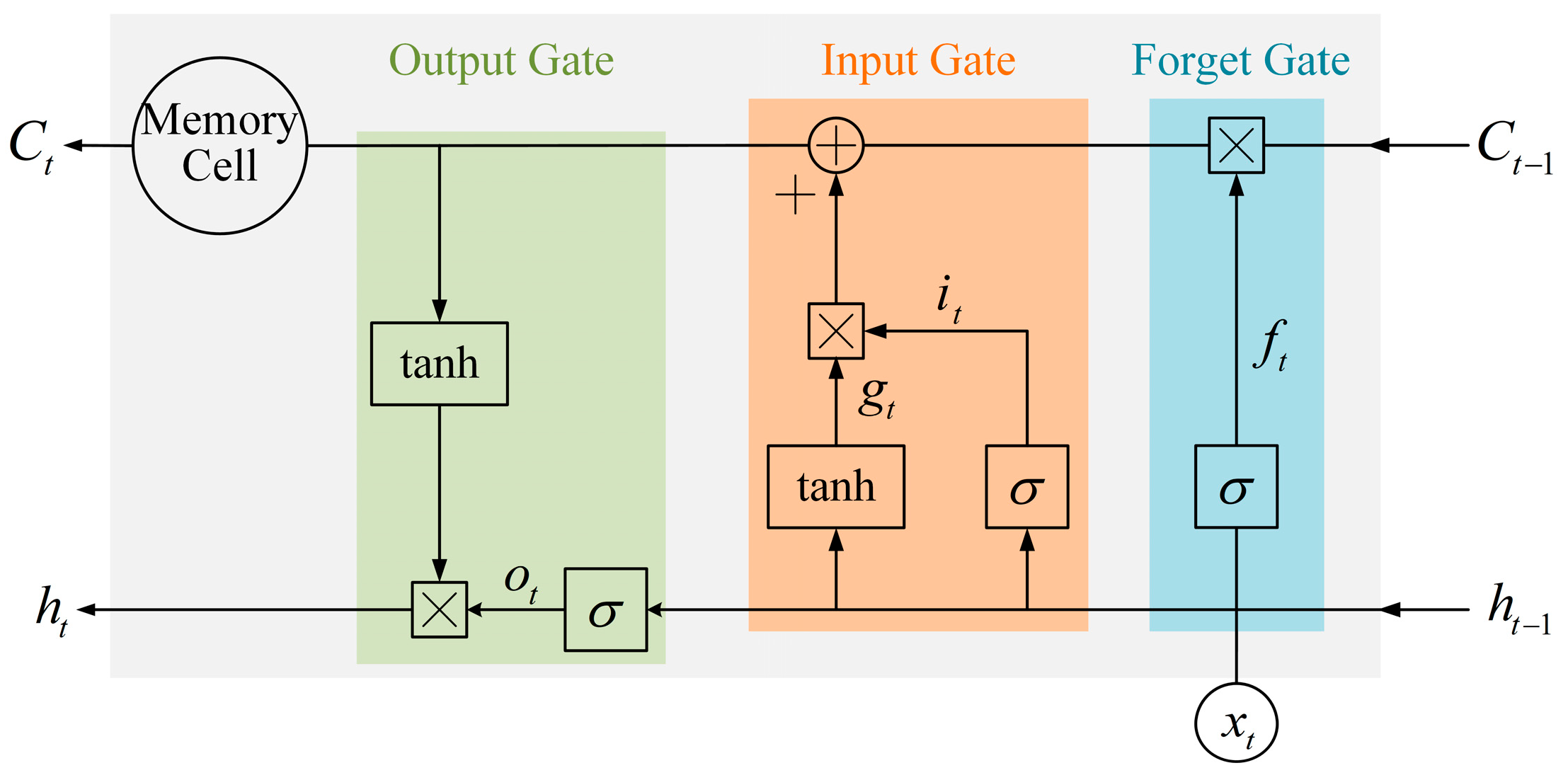
In order to identify the electricity consumption behavior of users in a distribution substation, the fuzzy C-means clustering algorithm (FCM) and genetic algorithm (GA) are combined for cluster analysis. FCM is a widely used local search fuzzy clustering algorithm [29], which realizes the clustering of sample data by calculating the membership degree of data and each cluster center, which can be defined as an optimization problem with a sample size of N, specifically as follows:

$$\left\{\begin{array}{l}\min J={\displaystyle \sum _{i=1}^N{\displaystyle \sum _{j=1}^c{u}_{ij}^M{‖{\mathit{x}}_i-{\mathit{c}}_j‖}^2}}\\ s.t.{\displaystyle \sum _{i=1}^N{u}_{ij}=1}\end{array}\right.$$

(1)

where c represents the number of cluster centers; M represents a fuzzy weighted index; X_i is the i-th sample; c_j is the j-th cluster center; and u_ij is the membership coefficient of sample x_i belonging to category j. The respective iterative calculation formulas for cluster center and membership coefficient are expressed as follows:

$$c_j={\displaystyle \frac{{\displaystyle \sum _{i=1}^N{u}_{ij}^M{\mathit{x}}_i}}{{\displaystyle \sum _{i=1}^N{u}_{ij}^M}}}$$

(2)

$$u_{ij}={\displaystyle \frac{1}{{\displaystyle \sum _{k=1}^c{\left(\frac{‖{\mathit{x}}_j-{\mathit{c}}_i‖}{‖{\mathit{x}}_j-{\mathit{c}}_k‖}\right)}^{\frac{2}{M-1}}}}}$$

(3)

The FCM algorithm has a fast convergence speed, but since it is based on the gradient descent method for optimization, it has the disadvantages of a high dependence on initial values and the tendency to become trapped in local optima, resulting in the inability to obtain accurate clustering results of electricity consumption characteristics. In order to solve the above problems, the GA algorithm is introduced to optimize the initial cluster centers of FCM [30]. The basic idea is to start the search process from an initial solution of a group of randomly generated populations, and each individual in the population corresponds to a solution to the problem. Offspring are produced by operations such as crossovers and mutations from the previous generation, and a selection process based on fitness values determines which offspring are retained or eliminated to maintain a constant population size. After several generations, the algorithm converges to the optimal individual, that is, the approximate solution of the global optimal solution is obtained. The FCM algorithm is further used to obtain the final classification results.

2.3. BiLSTM

BiLSTM is a time-based bidirectional recurrent neural network, which can effectively mine the intrinsic relationship between the current data and the past and future time data through forward time series and reverse time series training, and then make full use of the information of the load data [31]. The BiLSTM network is an improvement and optimization based on the LSTM network, which aims to solve the technical problem of the LSTM network due to one-way propagation, that is, when forecasting based on time series, the past and future sequence information cannot be used to evaluate the current moment. As shown in Figure 1, the neuronal structure of the LSTM network is mainly composed of a forget gate, an input gate, an output gate, and a memory cell.

During the training process of the LSTM network, the state c_t of the memory cell at time t is composed of a forgotten part and a retained part. The forgotten part is determined by the input x_t, the state c_t−1 of the memory cell at time (t − 1), and the intermediate output h_t. The reserved part of the state is jointly determined by the output of x_t after being transformed by the sigmoid function (σ) and the tanh function. Additionally, in the output gate, x_t and c_t are transformed to obtain h_t. The calculation formulas for each variable in Figure 1 are written as follows:

$$f_t=\sigma \left(W_f\times \left[h_{t-1},x_t\right]+b_f\right)$$

(4)

$$i_t=\sigma \left(W_i\times \left[h_{t-1},x_t\right]+b_i\right)$$

(5)

$$g_t=\tanh \left(W_g\times \left[h_{t-1},x_t\right]+b_g\right)$$

(6)

$$o_t=\sigma \left(W_o\times \left[h_{t-1},x_t\right]+b_o\right)$$

(7)

$$c_t=c_{t-1}\times f_t+g_t\times i_t$$

(8)

$$h_t=o_t\times \tanh \left(c_t\right)$$

(9)

where W_f is the weight matrix for the forgotten gate; W_i and W_g are the weight matrices for the input gate; W_o is the weight matrix for the output gate; b_f is the bias term for the forget gate; b_i and b_g are the bias terms for the input gate; and b_o is the bias term for the output gate.

The BiLSTM network is constructed by connecting two LSTMs, forming a forward propagation hidden layer and a backward propagation hidden layer. This creates a data flow from past to future and from future to past, enabling the output at the current time step to utilize information in both forward and reverse directions at the same time. Figure 2 shows the result of the BiLSTM model unfolding along the time axis, where $x^{\prime }$ is the model input, $h^{\prime }$ is the hidden layer state, and y is the model output.

Let $\overrightarrow{h_t^{\prime }}$ be the state of the forward propagation hidden layer at time t and $\overleftarrow{h_t^{\prime }}$ be the backward propagation hidden layer at time t, then

$$\overrightarrow{h_t^{\prime }}=\mathrm{LSTM}\left(x_t^{\prime },\overrightarrow{h_{t-1}^{\prime }}\right)$$

(10)

$$\overleftarrow{h_t^{\prime }}=\mathrm{LSTM}\left(x_t^{\prime },\overleftarrow{h_{t-1}^{\prime }}\right)$$

(11)

where LSTM represents the LSTM unit; $x_t^{\prime }$ is the input of time t; $\overrightarrow{h_{t-1}^{\prime }}$ is the state of the forward propagation hidden layer at time (t − 1); and $\overleftarrow{h_{t-1}^{\prime }}$ is the state of the backward propagation hidden layer at time (t − 1). By combining $\overrightarrow{h_t^{\prime }}$ and $\overleftarrow{h_t^{\prime }}$, the overall output state y_t of the BiLSTM network is formed.

3. Modeling of Distribution Substation Load Forecasting

3.1. Forecasting Model Architecture

As shown in Figure 3, the load forecasting model architecture is constructed using the aforementioned methods. The specific process is divided into the following two stages.

(1)

Analysis of the Characteristics of Influencing Factors.

PCA is used to extract the principal components of the high-dimensional external factor data and be input into the BiLSTM network for training. At the same time, the FCM algorithm is used to cluster the user electricity consumption data, the optimal initial clustering center is obtained based on the GA algorithm, and the user datasets of different electricity consumption behavior categories are obtained.

(2)

BiLSTM Forecasting Model Design.

Separate BiLSTM forecasting models are constructed for each category of users, and the stochastic weight averaging (SWA) algorithm is employed to optimize the network. For different categories of users in the target distribution substation, the corresponding PCA-BiLSTM models are used for forecasting. The predicted values of all users are aggregated to obtain the load forecasting result for the distribution substation.

3.2. Data Preprocessing

3.2.1. Data Characteristics

There are many factors influencing the load of the power system, with meteorological factors being the most prevalent [32]. Additionally, since the electricity load curve has obvious daily periodicity and weekly periodicity [33], it is necessary to consider the weather conditions and date types when making load forecasting. Moreover, historical load data conceal the electricity consumption behavior patterns of the users. Exploring these data and studying user types can contribute to a more comprehensive description of the substation system.

Based on the above analysis, the focus of this paper is on predicting daily electricity loads at the substation level, categorizing the influencing factors of the system into external factor features and electricity consumption behavior features. Moreover, incorporating substation losses and regional factors into load forecasting methodologies offers potential improvements in forecasting accuracy and model robustness. Future research should explore these factors across diverse geographical regions to validate and generalize the findings of this study.

(1)

Characteristics of external factors.

Nine characteristics of the forecast day, comprising maximum temperature, minimum temperature, average temperature of the day, average temperature of the previous day, humidity, precipitation, weather conditions (including 33 weather types such as sunny, cloudy, overcast, and shower), date type (day of the week), and month are selected as alternative inputs for the model. In addition, the model output is the daily load value for the next one day.

(2)

Characteristics of electricity consumption behavior.

By analyzing the shape characteristics of the electricity consumption curve of the users, the electricity consumption behavior is described. The shape of the electricity consumption curve is depicted from the three dimensions of fluctuation point, mean, and variance. The specific process is as follows: first, the random fluctuation component in the electricity consumption data is stripped by smoothing. Secondly, the reference peak electricity consumption tends to occur in summer and winter [34], and considering the operating efficiency of the system, the two fluctuation points with the largest change in the slope of the electricity consumption curve are selected, and the curve is divided into three segments. Then, calculate the average and variance in each segment of electricity consumption data after segmentation. Finally, the time series coordinate values of the two fluctuation points of the electricity consumption curve of each user, the average electricity consumption value of the three curves, and the variance in electricity consumption are taken as the characteristics of the electricity consumption behavior.

3.2.2. Missing Values

In order to ensure the correctness and objectivity of the forecasting results, in view of the missing value problem of the time series data, this paper combines the characteristics of the daily and weekly periodicity of the electricity load curve, and considers the time continuity of the load data, and adopts the method of mean data imputation, that is, the average number of daily electricity load values of a total of five sampling points 2 days before and after the missing value and 1 week ago is completed as follows:

$$L_{m,n}={\displaystyle \frac{L_{m-1,n}+L_{m,n-1}+L_{m,n-2}+L_{m,n+1}+L_{m,n+2}}{5}}$$

(12)

where $L_{m,n}$ represents the value of the electricity load on the n-th day of the m-th week.

3.2.3. Outliers

Outliers are caused by input errors, measurement errors, experimental errors, and other similar situations. When such data are included in the forecasting model training, they can lead to significant biases in the forecasting results. In this paper, box plot analysis is applied [35] to identify outlier data and validate them against the normal fluctuation range of electrical quantities in the distribution network. Once confirmed as outliers, these data points are treated as missing values and handled according to the methods for handling missing data.

3.3. Analysis of Influencing Factor Characteristics

3.3.1. External Factor Characteristic Dimensionality Reduction

According to the characteristics of the nine external factors selected in the data preprocessing process, the PCA method is used to reduce the data dimensionality. The specific steps are as follows.

Step 1: Represent the input variable dataset X of nine influencing factors with p load data samples as $X=\left[X_1,X_2,\dots ,X_9\right]$, where $X_i=\left[X_{1i},X_{2i},\dots ,X_{pi}\right]$. Then, the covariance matrix of X can be represented as follows:

$$S={\displaystyle \sum {\left(s_{ij}\right)}_{9\times 9}}$$

(13)

$$s_{ij}={\displaystyle \frac{1}{p-1}}{\displaystyle \sum _{k=1}^p\left(x_{ki}-{\overline{x}}_i\right)}\left(x_{kj}-{\overline{x}}_j\right)$$

(14)

where $i=1,2,\dots ,9$; $j=1,2,\dots ,9$; $\overline{x}$ is the average of x.

Step 2: Compute the eigenvalues and corresponding orthogonal unit eigenvectors of matrix S, and reorder the nine influencing factors based on their eigenvalues in descending order, resulting in a new eigenvalue sequence ${\lambda }_1,{\lambda }_2,\dots ,{\lambda }_9$ and eigenvector sequence ${\mu }_1,{\mu }_2,\dots ,{\mu }_9$.

Step 3: Calculate the variance contribution rate ${\eta }_r$ and the cumulative variance contribution rate ${\eta }_{\Sigma }\left(r\right)$ of the r-th input variable, which are expressed, respectively, as follows:

$${\eta }_r={\displaystyle \frac{{\lambda }_r}{{\displaystyle \sum _{k=1}^9{\lambda }_k}}}$$

(15)

$${\eta }_{\sum }\left(r\right)={\displaystyle \sum _{i=1}^r{\eta }_i}$$

(16)

When the cumulative variance contribution rate of the input variables exceeds 85%, it is considered that the first r influencing factors contain most of the information in the input variable dataset, that is, the principal components [36,37].

3.3.2. Feature Clustering of Electricity Consumption Behavior

In order to fully reflect the characteristics of users’ electricity consumption behavior and obtain objective classification results, when performing feature clustering analysis, the data should include the daily electricity load value of users in recent years. On this basis, the load data of each user are superimposed in annual intervals, and the average daily electricity load is obtained. Considering that the electricity consumption behavior has obvious weekly periodicity, the segmented aggregation approximation method with a sampling frequency of 7 days/time is used to smooth the data, and the sampling value represents the user’s electricity consumption in the previous week. Further, the GA-FCM method is further applied for feature clustering, and the steps are as follows.

Step 1: Initialize the parameters, including the initial number of cluster centers c, population size, cross probability, and iteration termination threshold T. On this basis, the binary gene string coding $\alpha =\left\{{\alpha }_1{\alpha }_2\dots {\alpha }_i\dots {\alpha }_q\right\}$ of the cluster center coordinates is performed, where each pair of values in $\alpha$ represents the coordinates of a cluster center, resulting in $q=c\times 2$.

Step 2: Randomly select the initial population and set the number of iterations $l=0$.

Step 3: Design the fitness function $f=1/\left(1+J\right)$ according to Equation (1) and calculate the individual fitness.

Step 4: Generate a new population through genetic operations (selection, crossover, mutation). Terminate the computation when the stopping iteration condition $‖c^{\left(l\right)}-c^{\left(l+1\right)}‖<T$ is met, otherwise, increment l by 1 and return to Step 2 to continue iterating until the stopping iteration condition is satisfied. Output the clustering results.

3.4. BiLSTM Forecasting Model Design

3.4.1. Forecasting Model Structure

In this paper, a BiLSTM forecasting model is built based on the built-in neural network structure under the Keras framework, with the programming environment set to Python 3.7. Third-party libraries such as NumPy, Pandas, Matplotlib, Keras, and Scikit-learn are utilized. Recognizing the issue of reduced prediction accuracy due to stochastic fluctuations in time series forecasting, the experiment constructs a two-layer BiLSTM network. This BiLSTM network is connected with a dense (fully connected) layer to extract the deeper level features.

Building upon this, the mean absolute percentage error (MAPE) is selected as the loss function whose calculation formula is shown as Equation (17) to predict the electricity load of each category of users. Further, by adding a dropout layer, the overfitting problem is solved. The model network structure is depicted in Figure 4.

$$\mathrm{MAPE}={\displaystyle \frac{1}{n_f}}{\displaystyle \sum _{i=1}^{n_f}\frac{\left|\left.y_i-\widehat{y_i}\right|\right.}{y_i}}\times 100\%$$

(17)

where $n_f$ is the number of load forecast points, and $y_i$, $\widehat{y_i}$ are the true value and forecast value for the i-th load forecasting point, respectively.

The architecture of our model is structured with the first and second layers consisting of BiLSTM units, each initialized with 128 neurons and utilizing the ReLU activation function. These choices are informed by established practices in natural language processing for effectively capturing sequential dependencies. The third layer is a fully connected layer with 64 neurons and a ReLU activation function, aimed at integrating features extracted from the preceding BiLSTM layers. The fourth layer incorporates a dropout mechanism with a dropout probability of 0.3, which helps mitigate overfitting by randomly dropping neuron nodes during training. The final layer serves as the output layer with a dimensionality of one, employing the ReLU activation function to produce the final predictions.

The selection of these specific parameter values was guided by a hybrid approach combining insights from the literature review and empirical experimentation. The initial neuron count of 128 in the BiLSTM layers, for instance, aligns with recommended settings for handling sequential data. Similarly, the use of ReLU activation functions throughout the network is standard practice due to their effectiveness in avoiding the vanishing gradient problem. The choice of a dropout probability of 0.3 was determined through iterative testing to balance model complexity and generalization performance.

3.4.2. SWA Optimization Algorithm

In our study, we opted for stochastic gradient descent (SGD) as the baseline optimizer due to its simplicity and well-established effectiveness in optimizing deep neural networks across various domains. This choice was motivated by the need to maintain a stable learning trajectory, particularly given the complexity of our experimental setup. Building upon SGD, we explored stochastic weight averaging SGD (SWA-SGD), which involves averaging weight vectors during the optimization process. Recent studies have demonstrated that SWA-SGD can enhance generalization performance and robustness by smoothing out the trajectory of SGD. While optimization methods like adaptive moment estimation (Adam) offer adaptive learning rates and momentum terms, which may accelerate convergence in certain scenarios, we chose to focus on SGD and SWA-SGD for their specific benefits in our experimental context.

The typical training process of a deep learning network involves optimizing the loss function using an optimizer with a decaying learning rate until the model converges. In the model training process, using the stochastic gradient descent (SGD) optimizer and during each parameter update round, a random sample or subset is used to compute gradients, which serve as estimates of the global gradients. However, due to noise in the real data, the SGD optimizer often struggles to approach the optimal parameters along the best update direction, leading to frequent parameter updates and oscillations in the loss function, which can impact the accuracy of load forecasting.

To address these issues, this paper applies the SWA algorithm to improve the SGD optimizer and further enhance the model’s generalization ability. The SWA algorithm, built upon the SGD optimizer, incorporates periodic sliding average operations that limit weight changes, i.e., averaging the network weights traversed by the SGD optimizer. This limitation reduces the frequency of parameter updates and facilitates easier identification of optimal value ranges [38,39]. The specific optimization steps are as follows:

Step 1: set the pre-training weight $W_{\mathrm{SWA}}=\widehat{\omega }$ and start training based on the SGD optimizer;

Step 2: during the training process, the sliding average $W_{\mathrm{SWA}}$ with a period of $\theta$, that is, every iteration, computes the weighted average of the model parameters and updates $W_{\mathrm{SWA}}$;

Step 3: apply the updated $W_{\mathrm{SWA}}$ for gradient descent training and repeat Step 2 until the model converges.

4. Example Analysis

In this study, the electricity load data are analyzed, collected from a low-voltage distribution substation in China servicing 174 users from 2018 to 2021. The users encompass diverse categories including residential and commercial, situated across various building types. This research employs methodologies for integrating electricity consumption feature clustering and PCA-BiLSTM for forecasting.

Table 1. Load power of the distribution substation.

Year	Maximum Power/kW	Minimum Power/kW
2018	488.890	151.792
2019	524.355	183.294
2020	501.634	157.415
2021	519.181	180.428

presents the annual maximum and minimum power levels recorded at the substation. The data reveal fluctuations across the study period, notably with a peak in 2019 followed by a decline in 2020 and a subsequent slight increase in 2021 (see Table 1). These variations may reflect broader economic or seasonal factors influencing electricity consumption patterns among different user categories. While our initial analysis suggested a minimal direct impact of the COVID-19 pandemic on the overall load, these observations prompt further exploration into the underlying dynamics driving these fluctuations.

During the experimental process, each year from 1 January to 31 December is considered as one cycle. Historical load data from 2018 to 2020 are selected as the training set to establish the distribution substation load forecasting models. Historical load data from 2021 are chosen as the test set to evaluate the forecasting performance. Furthermore, MAPE and root mean square percentage error (RMSPE) are utilized as the evaluation metrics to compare the prediction accuracy of the LSTM model, BiLSTM model, and PCA-BiLSTM model, aiming to validate the effectiveness of the proposed forecasting method. These scale-invariant measures are well-suited for assessing the predictive performance across diverse datasets, providing insights into percentage-wise and squared percentage-wise errors, respectively. The calculation formula for RMSPE is written as follows:

$$\mathrm{RMSPE}=\sqrt{{\displaystyle \frac{1}{n_f}}{{\displaystyle \sum _{i=1}^{n_f}\left(\frac{\left|\left.y_i-\widehat{y_i}\right|\right.}{y_i}\right)}}^2}\times 100\%$$

(18)

While our study focused on MAPE and RMSPE for their consistency and interpretability across various conditions, future investigations could benefit from integrating scale-dependent metrics like mean absolute error (MAE) and root mean square error (RMSE). These metrics capture absolute differences, offering complementary insights, particularly in contexts sensitive to data variability and magnitude. Exploring the inclusion of MAE, RMSE, or other scale-dependent metrics in future work would enrich our understanding of prediction performance, especially where absolute error magnitudes are critical. This approach would contribute to a more nuanced evaluation framework, enhancing the robustness and applicability of our findings.

4.1. Input Variable Selection

The results of extracting the principal components of the four load-influencing factors based on the PCA method are shown in

Table 2. Principal component extraction results.

Principal Component	Eigenvalue	Variance Contribution/%	Cumulative Variance Contribution/%
1	12.782	29.491	29.491
2	10.433	24.071	53.562
3	8.365	19.300	71.862
4	5.964	13.760	86.622

. The cumulative contribution of Principal Component 1 to Principal Component 4 reaches 86.622%, which already contains most of the information of the loaded impact factors. The external factor characteristics with the largest weight coefficient among the four principal components are the average temperature of the forecast day, the date type, the weather condition, and the month. Therefore, these four principal components can replace the original set of nine features as input variables for training the BiLSTM forecasting model. This approach achieves feature dimensionality reduction, thereby enhancing the efficiency of the algorithm.

4.2. Classification of Electricity Consumption Behavior

The daily average load for each user over 3 years is calculated based on historical load data from 2018 to 2020. Furthermore, the weekly electricity consumption data are obtained through down-sampling. Considering the significant differences in electricity consumption levels among different users, the weekly electricity consumption data are normalized as follows:

$$z_{i,t}={\displaystyle \frac{co{n}_{i,t}}{co{n}_{i,\max }}}$$

(19)

where $z_{i,t}$ represents the normalized data of the sampled values of the user i at time t; $co{n}_{i,t}$ is the weekly electricity consumption of the user i at time t; and $co{n}_{i,\max }$ is the maximum weekly electricity consumption of the user i over the year.

The GA-FCM method is applied to perform feature clustering on the normalized data, resulting in three typical user groups. Figure 5 displays the weekly average electricity consumption curves for each user group, highlighting distinct differences in electricity consumption patterns among the three groups, characterized by seasonal fluctuations.

4.3. Experimental Results Analysis

In this experiment, daily cumulative loads for each user category from 2018 to 2020 are selected as the training sets for their respective forecasting models. Further application of these forecasting models is used to forecast the daily cumulative loads of all users in each user category for 2021.

4.3.1. Analysis of BiLSTM Forecasting Model

To evaluate the effectiveness of the two-layer BiLSTM network, single-layer and two-layer BiLSTM networks are separately trained using the training set. The models are optimized using SGD. Furthermore, the training process is compared based on the loss of the training set after each iteration, as shown in Figure 6. The loss of the validation set is also plotted in Figure 6, and it can be found that the validation set is closer to the training set, which solves the overfitting problem better. It can be observed that both network structures significantly reduced the loss values after 150 iterations. By 600 iterations, the loss values had stabilized. Additionally, the two-layer BiLSTM network consistently exhibited lower loss values, demonstrating superior forecasting performance.

In addition, the SWA algorithm is further applied to optimize the forecasting model based on the bilayer BiLSTM network. During the training process, when the iteration reaches 500 times, the loss value tends to be stable, showing better generalization ability.

4.3.2. User Load Forecasting Results

For the three user categories, the LSTM, BiLSTM, and PCA-BiLSTM forecasting models are constructed using a five-layer neural network structure with identical layer parameters and trained for 500 iterations. The load forecasting results and performance metrics comparison for the three models are shown in Figure 7 and

Table 3. Valuation metrics of load forecasting for category 1.

Evaluation Metric	LSTM/%	BiLSTM/%	PCA-BiLSTM/%
MAPE	13.29	6.69	5.61
RMSPE	17.56	12.31	8.93

,

Table 4. Valuation metrics of load forecasting for category 2.

Evaluation Metric	LSTM/%	BiLSTM/%	PCA-BiLSTM/%
MAPE	12.18	5.80	5.56
RMSPE	15.73	11.08	8.87

and

Table 5. Valuation metrics of load forecasting for category 3.

Evaluation Metric	LSTM/%	BiLSTM/%	PCA-BiLSTM/%
MAPE	12.44	7.01	5.43
RMSPE	16.41	12.39	8.79

.

From Table 3, Table 4 and Table 5, it can be observed that compared to the LSTM model, both the BiLSTM and PCA-BiLSTM models closely approximate the actual load values, accurately reflecting the daily electricity consumption of the three user categories throughout the year. Furthermore, error analysis data and comparison of the BiLSTM model’s forecasting results show significant reductions in MAPE and RMSPE metrics for the PCA-BiLSTM model across all three user categories. This further highlights the significant improvement in forecasting performance achieved by the PCA method. By reducing the data dimensions effectively, the PCA-BiLSTM model enhances load forecasting accuracy.

Following further analysis of the electricity load curves of the three categories of users, the corresponding electricity consumption behavior characteristics are obtained as follows.

(1)

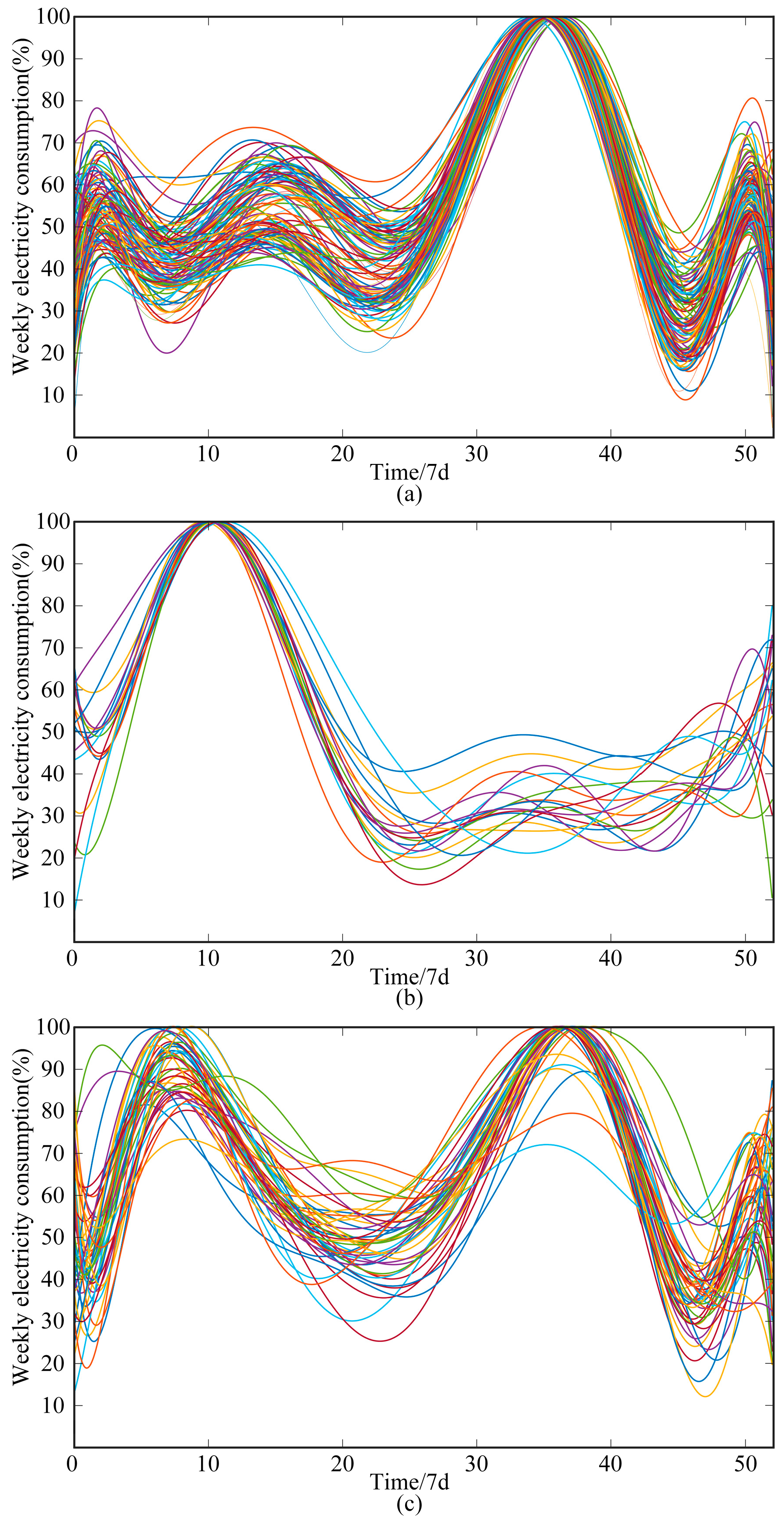
As shown in Figure 7a, the electricity load curve of the first type of user is unimodal in summer. The electricity consumption has a significant peak in July and August, and the electricity consumption in other periods is relatively stable. Combined with the regional climate characteristics, it is inferred that such users use air conditioners and other electrical equipment in a large area in summer, so the demand for electricity and cooling is high. However, the demand for electricity heating in winter is small. This category can correspond to residential users with better heating effects in winter in the substation.

(2)

As shown in Figure 7b, the electricity load curve of the second type is unimodal in the winter–spring alternating season. The electricity consumption peaks in February and March, and the fluctuation of electricity consumption in other seasons is small. It is inferred that after the end of the winter central heating period, this category has a surge in electricity heating consumption due to poor house insulation.

(3)

As shown in Figure 7c, the electricity load curve of the third type is bimodal. There is a peak in the winter–spring season and the summer months, and the peak period of summer electricity demand is more concentrated. According to this, it is inferred that the electricity demand for summer cooling and winter heating of this category is large.

4.3.3. User Load Forecasting Results

The PCA-BiLSTM model forecasting results of the above three categories of users are linearly superimposed to obtain the 2021 load forecasting data of the selected substation. A comparison is then made with the PCA-BiLSTM model results that do not distinguish between electricity consumption behavior categories as shown in Figure 8. According to Equations (17) and (18), the calculated MAPE for the differentiated electricity consumption category prediction within the 52-week (364-day) period for the selected substation is 5.65%, with an RMSPE of 7.89%. In contrast, the MAPE for the undifferentiated electricity consumption category results is 6.22%, with an RMSPE of 10.57%. It can be observed that distinguishing between electricity consumption behavior categories for all users in the substation, constructing PCA-BiLSTM models accordingly, and aggregating the results yield higher forecasting accuracy. Therefore, analyzing different types of electricity consumption behavior within the substation can help in formulating more targeted plans for power operations, maintenance, and other related activities.

4.4. Comparison with Existing Literature

Our study introduces a novel short-term load forecasting method for low-voltage distribution substations using the BiLSTM model enhanced with the stochastic weight averaging (SWA) algorithm. This approach integrates principal component analysis (PCA) and GA-FCM-based fuzzy C-means to classify user electricity consumption behaviors, thereby enhancing feature extraction and model generalization. Comparatively, the existing literature has explored the following different methodologies:

Chapagain et al. [16] enhanced traditional Bayesian forecasting models to improve generalization and achieve high prediction accuracy. However, these methods may face computational inefficiencies under complex influencing factors. Zhang et al. [19] improved the support vector machine regression (SVR) algorithm, known for its maturity in quickly attaining global optima but heavily reliant on historical data, potentially affecting accuracy during load fluctuations. Dong et al. [23] utilized pre-trained weight values in restricted Boltzmann machines to enhance the load forecasting accuracy using forward neural network models. These methods demonstrate high precision but have been critiqued for slow convergence, poor model interpretability, and susceptibility to overfitting.

In contrast, our PCA-BiLSTM-SWA model demonstrates superior accuracy in forecasting annual electricity load curves across various user types compared to conventional LSTM and BiLSTM models. By leveraging SWA, our model improves robustness against overfitting and enhances generalization capabilities, making it suitable for real-time forecasting scenarios.

5. Conclusions

In this paper, the GA-FCM algorithm is applied to classify electricity consumption behaviors among three typical categories of users in low-voltage substations. It utilizes PCA to extract the four influential factors affecting electricity load as feature inputs for the forecasting model. Based on this foundation, BiLSTM models are constructed to forecast the short-term electricity loads of each user category, thereby obtaining the overall load profiles of the distribution substation. The conclusions of the analysis and verification are as follows.

(1)

A certain correlation among various influencing factors of electricity load exists in the low-voltage substation. By recombining the influencing factors, four principal component variables can be formed to describe the external factor system that affects electricity consumption.

(2)

Significant differences exist in electricity consumption behaviors among users in the low-voltage substation. Based on the weekly electricity load curves of each user class, these behaviors can be categorized into three types: summer peak, winter–spring single peak, and double peak.

(3)

Compared to the LSTM and BiLSTM models, the PCA-BiLSTM model demonstrates a higher accuracy in load forecasting, which can accurately reflect the electricity consumption behaviors of various user categories in the low-voltage substation. The classification forecasting method based on electricity consumption behavior analysis effectively enhances the accuracy of forecasting results, demonstrating a practical application value.

This study employs data sourced from a specific region’s electricity information collection system to validate the effectiveness of the proposed algorithm. The selection of this dataset was motivated by its availability and suitability for demonstrating the practical application of the BiLSTM model enhanced with the SWA algorithm in short-term load forecasting. While the chosen data source serves to validate our methodology within the studied region, we acknowledge that its regional specificity may limit the generalizability of our findings to areas with diverse socio-economic conditions, weather patterns, and electricity consumption behaviors. To mitigate this limitation, future research endeavors could focus on validating our approach across various data sources from different geographical locations. Future work will integrate load data from different regions and consider substation losses to further analyze electricity consumption behavior and external factor characteristics, achieving more accurate load forecasting to enhance the efficient operation of the power grid.

References

1. Qiu, Z.T.; Han, X.Y.; Tian, X.; Zhu, R. Research on collaborative needs and typical scenarios of smart distribution network assisting modern infrastructure construction. Distrib. Util. 2024, 41, 47–54. [Google Scholar]
2. Yang, X.Y.; Li, S.J. Design of distribution network operation safety monitoring system based on electric power big data and portrait. Electron. Des. Eng. 2023, 31, 54–57+62. [Google Scholar]
3. Kong, X.Y.; Ma, Y.Y.; Ai, Q.; Zhang, X.Y.; Li, C.; Xiao, B. Review on Electricity Consumption Characteristic Modeling and Load Forecasting for Diverse Users in New Power System. Autom. Electr. Power Syst. 2023, 47, 2–17. [Google Scholar]
4. Lin, J.; Ma, J.; Zhu, J.; Cui, Y. Short-term load forecasting based on LSTM networks considering attention mechanism. Int. J. Electr. Power Energy Syst. 2022, 137, 107818. [Google Scholar] [CrossRef]
5. Hong, T.; Fan, S. Probabilistic electric load forecasting: A tutorial review. Int. J. Forecast. 2016, 32, 914–938. [Google Scholar] [CrossRef]
6. Li, P.; Xi, W.; Cai, T.T.; Yu, H.; Li, P.; Wang, C.S. Concept, architecture and key technologies of digital power grids. Proc. CSEE 2022, 42, 5002–5016. [Google Scholar]
7. Zhou, X.X.; Chen, S.Y.; Lu, Z.X.; Huang, Y.H.; Ma, S.C.; Zhao, Q. Technology Features of the New Generation Power System in China. Proc. CSEE 2018, 38, 1893–1904+2205. [Google Scholar]
8. Song, K.B.; Baek, Y.S.; Hong, D.H.; Jang, G. Short-term load forecasting for the holidays using fuzzy linear regression method. IEEE Trans. Power Syst. 2005, 20, 96–101. [Google Scholar] [CrossRef]
9. Bunnoon, P.; Chalermyanont, K.; Limsakul, C. Mid term load forecasting of the country using statistical methodology: Case study in Thailand. In Proceedings of the International Conference on Signal Processing Systems, Singapore, 15–17 May 2009; pp. 924–928. [Google Scholar]
10. Lei, S.L.; Sun, C.X.; Zhou, Q.; Zhang, X.X. The research of local linear model of short term electrical load on multivariate time series. In Proceedings of the IEEE Russia Power Tech, St. Petersburg, Russia, 27–30 June 2005; pp. 1–5. [Google Scholar]
11. Soares, L.J.; Medeiros, M.C. Modeling and forecasting short-term electricity load: A comparison of methods with an application to Brazilian data. Int. J. Forecast. 2008, 24, 630–644. [Google Scholar] [CrossRef]
12. Tao, Y.; He, L.; Zhang, H.; Wang, X. Research on the prediction of fatigue life of tower crane based on grey system. Mech. Sci. Technol. Aerosp. Eng. 2012, 31, 1236–1240. [Google Scholar]
13. Wang, Q.; Li, S.; Li, R. Forecasting energy demand in China and India: Using single-linear, hybrid-linear, and non-linear time series forecast techniques. Energy 2018, 161, 821–831. [Google Scholar] [CrossRef]
14. Ma, J.; Yang, H.G. Application of adaptive kalman filter in power system short-term load forecasting. Power Syst. Technol. 2005, 29, 75–79. [Google Scholar]
15. Guan, C.; Luh, P.B.; Michel, L.D.; Chi, Z. Hybrid Kalman filters for very short-term load forecasting and prediction interval estimation. IEEE Trans. Power Syst. 2013, 28, 3806–3817. [Google Scholar] [CrossRef]
16. Chapagain, K.; Kittipiyakul, S. Short-term electricity load forecasting model and Bayesian estimation for Thailand data. In Proceedings of the Asia Conference on Power and Electrical Engineering (ACPEE), Bangkok, Thailand, 20–22 March 2016. [Google Scholar]
17. Jiang, W.; Huang, L.L.; Feng, W.; Yang, L.; Wang, L.; Xu, Q.S.; Wu, J.; Yang, H.B. Research on load forecasting technology of transformer areas based on distributed graph computing. Proc. CSEE 2018, 38, 3419–3430. [Google Scholar]
18. Xi, Y.W.; Wu, J.Y.; Shi, C.; Zhu, X.W.; Cai, R. A refined load forecasting based on historical data and real-time influencing factors. Power Syst. Prot. Control 2019, 47, 80–87. [Google Scholar]
19. Zhang, Z.; Hong, W.C. Application of variational mode decomposition and chaotic grey wolf optimizer with support vector regression for forecasting electric loads. Knowl.-Based Syst. 2021, 228, 107297. [Google Scholar] [CrossRef]
20. Dong, S.; Wang, P.; Abbas, K. A survey on deep learning and its applications. Comput. Sci. Rev. 2021, 40, 100379. [Google Scholar] [CrossRef]
21. Bedi, J.; Toshniwal, D. Deep learning framework to forecast electricity demand. Appl. Energy 2019, 238, 1312–1326. [Google Scholar] [CrossRef]
22. Sha, F.; Zhu, F.; Guo, S.N.; Gao, J.T. Based on the EMD and PSO-BP neural network of short-term load forecasting. Adv. Mater. Res. 2012, 614, 1872–1875. [Google Scholar] [CrossRef]
23. Dong, Y.; Dong, Z.; Zhao, T.; Li, Z.; Ding, Z. Short term load forecasting with markovian switching distributed deep belief networks. Int. J. Electr. Power Energy Syst. 2021, 130, 106942. [Google Scholar] [CrossRef]
24. Ciechulski, T.; Osowski, S. High precision LSTM model for short-time load forecasting in power systems. Energies 2021, 14, 2983. [Google Scholar] [CrossRef]
25. Zheng, J.; Xu, C.; Zhang, Z.; Li, X. Electric load forecasting in smart grids using long-short-term-memory based recurrent neural network. In Proceedings of the 51st Annual Conference on Information Sciences and Systems (CISS), Baltimore, MD, USA, 22–24 March 2017; pp. 1–6. [Google Scholar]
26. Ding, B.; Xing, Z.K.; Wang, F.; Yuan, B.; Liu, Y.; Sun, Y. Short-term load forecasting of LSTM network based on Stacking model integration. China Meas. Test 2020, 46, 40–45. [Google Scholar]
27. Wu, K.; Wu, J.; Feng, L.; Yang, B.; Liang, R.; Yang, S.; Zhao, R. An attention-based CNN-LSTM-BiLSTM model for short-term electric load forecasting in integrated energy system. Int. Trans. Electr. Energy Syst. 2021, 31, e12637. [Google Scholar] [CrossRef]
28. Shi, H.B. Power Load Forecasting Based on Principal Component Analysis and Support Vector Machine. Comput. Simul. 2010, 27, 279–282. [Google Scholar]
29. Bian, H.; Zhong, Y.; Sun, J.; Shi, F. Study on power consumption load forecast based on K-means clustering and FCM–BP model. Energy Rep. 2020, 6, 693–700. [Google Scholar] [CrossRef]
30. Zhang, L.; Lu, W.; Liu, X.; Pedrycz, W.; Zhong, C.; Wang, L. A global clustering approach using hybrid optimization for incomplete data based on interval reconstruction of missing value. Int. J. Intell. Syst. 2016, 31, 297–313. [Google Scholar] [CrossRef]
31. Varadharajan, S.K.; Nallasamy, V. P-SCADA—A novel area and energy efficient FPGA architectures for LSTM prediction of heart arrthymias in BIoT applications. Expert Syst. 2022, 39, e12687. [Google Scholar] [CrossRef]
32. Li, B.; Lu, M.Z. Short-term load forecasting modeling of regional power grid considering real-time meteorological coupling effect. Autom. Electr. Power Syst. 2020, 44, 60–68. [Google Scholar]
33. Dong, Y.; Ma, X.; Ma, C.; Wang, J. Research and application of a hybrid forecasting model based on data decomposition for electrical load forecasting. Energies 2016, 9, 1050. [Google Scholar] [CrossRef]
34. Wang, C.L.; Zheng, H.Y. A portrait of electricity consumption behavior mode of power users based on fuzzy clustering. Electr. Meas. Instrum. 2018, 55, 77–81. [Google Scholar]
35. Xu, M.; Liu, Z.C.; Yan, X.; Huang, B.X.; Wang, Y.; Wang, J.G. Online detection method for incremental capacity internal resistance consistency. Energy Storage Sci. Technol. 2019, 8, 1197–1203. [Google Scholar]
36. Chen, T.; Wang, Y.C. Long-term load forecasting by a collaborative fuzzy-neural approach. Int. J. Electr. Power Energy Syst. 2012, 43, 454–464. [Google Scholar] [CrossRef]
37. Afshar, K.; Bigdeli, N. Data analysis and short term load forecasting in Iran electricity market using singular spectral analysis (SSA). Energy 2011, 36, 2620–2627. [Google Scholar] [CrossRef]
38. Jiang, Z.H.; Wang, Y.X.; Yan, J.J.; Zhou, T.R. Modeling and analysis of cotton price forecast based on BILSTM. J. Chin. Agric. Mech. 2021, 42, 151–160. [Google Scholar]
39. Hu, Q.; Zhang, S.; Yu, M.; Xie, Z. Short-term wind speed or power forecasting with heteroscedastic support vector regression. IEEE Trans. Sustain. Energy 2015, 7, 241–249. [Google Scholar] [CrossRef]
Figure 1. Neuron structure of LSTM network.
Electronics 13 03098 g001
Figure 2. The structure of the BiLSTM network.
Electronics 13 03098 g002
Figure 3. Framework of the load forecasting model for the transformer district.
Electronics 13 03098 g003
Figure 4. Structure of the BiLSTM forecasting model.
Electronics 13 03098 g004
Figure 5. Clustering results of electricity consumption behavior characteristics: (a) Category 1 electricity consumption behavior of 109 users; (b) category 2 electricity consumption behavior of 18 users; (c) category 3 electricity consumption behavior of 47 users.
Electronics 13 03098 g005
Figure 6. Training set loss and validation set loss of the forecasting model.
Electronics 13 03098 g006
Figure 7. Load forecasting results: (a) Category 1 electricity consumption behavior; (b) category 2 electricity consumption behavior; (c) category 3 electricity consumption behavior.
Electronics 13 03098 g007
Figure 8. Load forecasting results of the distribution substation.
Electronics 13 03098 g008