Electromagnetic Fields Calculation and Optimization of Structural Parameters for Axial and Radial Helical Air-Core Inductors

Abstract

To improve the current density distribution and electromagnetic performance of air-core inductors, a structural optimization method combining back-propagation(BP) neural network and genetic algorithm(GA) is proposed for the study of axial and radial spiral multi-winding inductors. The Monte Carlo method was used to extract the structural size samples of the inductors, and the training dataset was obtained through the finite element calculation of electromagnetic fields. Based on BP neural networks, nonlinear mapping models between the inductance value, volumetric inductance density, current distribution non-uniformity coefficient, and inductor structural parameters were constructed. A sensitivity analysis of the inductor inductance value affected by the structural parameters was conducted using the Sobol index calculation. Using the current distribution non-uniformity coefficient as the fitness function and the volumetric inductance density as the constraint condition, a genetic algorithm was applied to globally optimize the structural parameters of the inductor. The optimization results were verified through a finite element comparison. The results show that, under the requirement of satisfying the volumetric inductance density, the current distribution non-uniformity coefficient of the Axial Helical Inductor (AHI)-type inductor was reduced by 4.57% compared with the best sample in the sampling, while that of the Radial Helical Inductor (RHI)-type inductor was reduced by 5.33%, demonstrating the practicality of the BP-GA joint algorithm in the structural optimization design of inductors.

1. Introduction

Inductors are devices used in power systems for current limiting, voltage stabilization, and reactive power compensation. Common inductors include air-core inductors, iron-core inductors, dry-type inductors, and oil-immersed inductors [1]. Dry-type air-core inductors are widely used in power systems due to their simple structure, low loss, good inductance linearity, absence of magnetic saturation, and ease of installation and maintenance [2,3]. As the core parameter of an inductor, the inductance has a decisive impact on its magnetic field distribution and performance. Meanwhile, the accuracy of the magnetic field calculations is directly related to the inductor’s performance evaluation and design precision. Therefore, accurately calculating the inductance and magnetic field of the inductor is crucial for ensuring stable operation of the power system [4,5].

Currently, there are two main methods for calculating the inductance and magnetic field of inductors: the analytical method and the finite element method [6]. To calculate single-winding inductors, Hao et al. [7] used analytical methods to investigate the magnetic field and inductance characteristics of inductors in pulsed power supplies, revealing the influence of shape ratios on inductor performance. Liu et al. [8] proposed analytical expressions representing performance parameters with structural parameters, improving the efficiency and parameter range of inductance calculations. Jiang et al. [9] employed the finite volume method to establish a calculation model for electromagnetic field loss and temperature rise in dry-type air-core inductors. To calculate the magnetic fields and inductances in multi-winding inductors, it is necessary to calculate the self-inductance and mutual inductance of each winding [10]. The derivation process using analytical methods can be complex and requires a certain degree of simplification, resulting in lower accuracy. Especially for inductors with special-shaped structures or iron cores, the calculation difficulty using analytical methods increases significantly.

Given the limitations of analytical methods in analyzing the magnetic field and inductance of inductors, the finite element method has gained attention due to its ability to flexibly handle various complex geometries and material properties, as well as its good adaptability to nonlinear problems and complex boundary conditions. Liu [11] and Gan [12] et al. used finite element software to establish field-circuit coupling models of air-core inductors. The former calculated the magnetic field and inductance of the inductor, while the latter analyzed the electromagnetic field and electromagnetic force distribution under steady-state conditions. Lin [13] utilized the finite element method to study the magnetic field and temperature field of dry-type air-core inductors, analyzing the loss distribution and temperature characteristics of the inductor. Ye et al. [14] proposed calculation the methods for 2D and 3D winding inductances of air-core inductors and verified their accuracy using finite element analysis. Most of the studies focus on model construction and the presentation of calculation results. However, there remains a lack of thorough examination of the spatial magnetic field distribution characteristics and systematic research on the influencing factors of inductance values for specific types of inductors, such as air-core inductors, which necessitates further exploration.

To further enhance the performance of inductors in power systems and meet the requirements for the stable operation of inductors under complex conditions, the structural optimization design of inductors is particularly important. Tan et al. [15] conducted a structural optimization design on controllable inductors with taps, proposing an optimization scheme that divides a single winding into inner and outer windings to seek the structural parameters for optimal impedance. Li et al. [16] comprehensively considered the temperature rise and structural strength requirements during the continuous operation of inductors. They optimized the structure of pulse inductors for electromagnetic launch by comparing the effects of different fixing methods and cooling methods on the stress and temperature of the inductor. With the goal of maximizing the energy density, Sun [17] and Li [18] et al. used genetic algorithms to optimize the design of toroidal air-core inductors and compiled an optimization program that can adjust the structural parameters of the inductor under given constraints to find samples with the maximum energy density, seeking the optimal structural parameters for inductors in induction pulse power supplies.

To improve the current density distribution and electromagnetic performance of air-core inductors, this paper considers axial spiral and radial spiral multi-winding inductors as the research objects and proposes a method for optimizing the inductor structure by combining a BP neural network with a genetic algorithm. The Monte Carlo method is used to extract samples of inductor structural dimensions, and the training dataset is obtained through parametric finite element calculations of electromagnetic fields. Based on BP neural networks, nonlinear mapping models between the inductance value, volumetric inductance density, current distribution non-uniformity coefficient, and inductor structural parameters were constructed. After that, Sobol index calculations are performed to analyze the parameter sensitivity of the inductor’s inductance value. A genetic algorithm is used to perform global optimization of the inductor’s structural parameters, and the optimization results are verified through finite element comparisons. This research provides more reliable theoretical foundations and data support for the optimized design of air-core inductors.

2. Finite Element Calculation of Electromagnetic Field for Air-Core Inductors

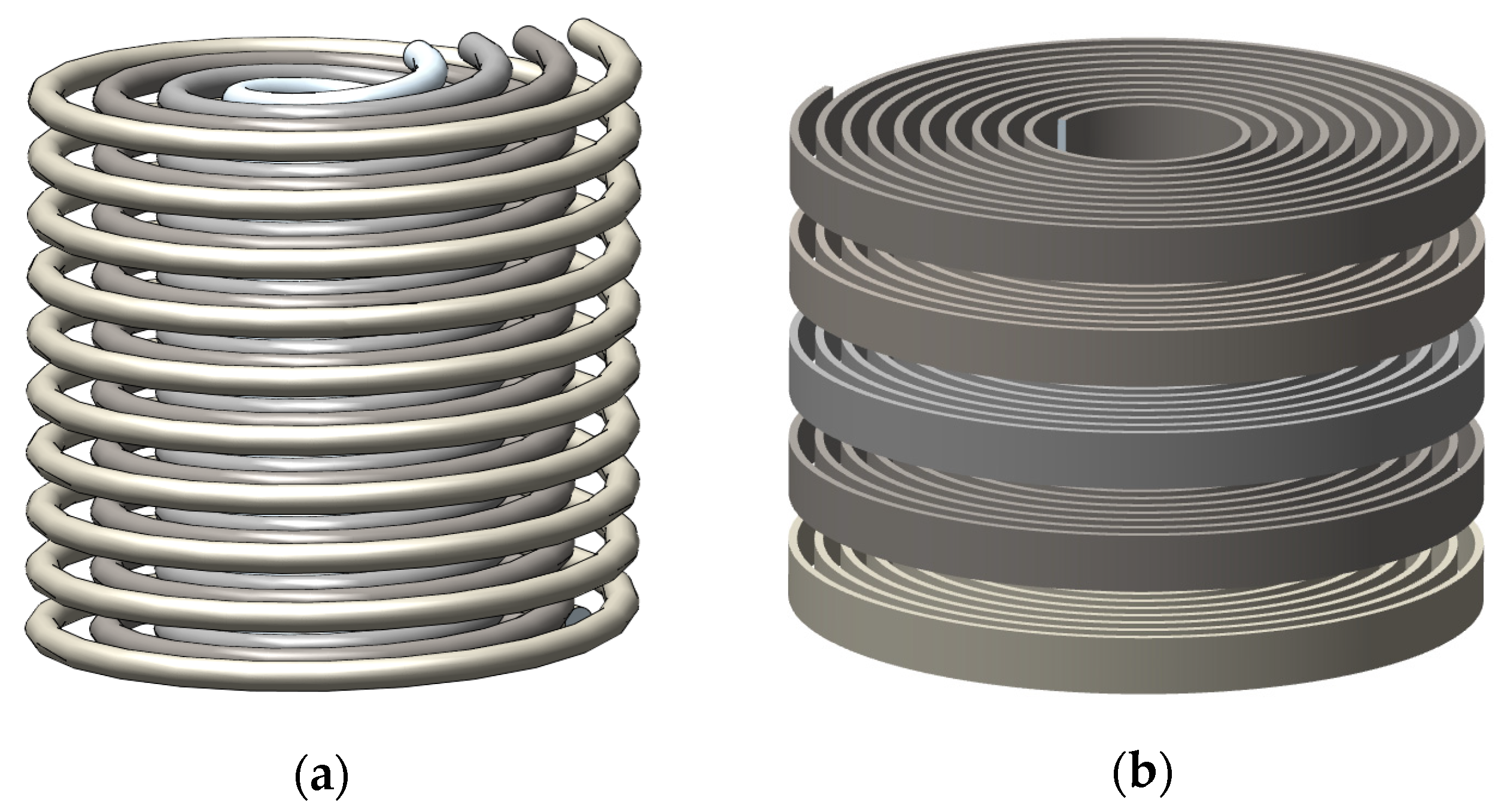
2.1. Two Types of Inductor Structures

The primary components of dry-type air-core inductors are coils, star frames, and support strips [19]. Coils are made of multiple envelopes connected in parallel. Each coil envelope is solidified into a single unit using glass fiber impregnated with epoxy resin, and insulation support strips made of epoxy resin are placed between the encapsulations to form heat dissipation channels. This paper compares two basic configurations of air-core inductors: the Axial Helical Inductor (AHI) and the Radial Helical Inductor (RHI), which are intended for capacitor energy storage-type pulse power supply. Their main functions are to adjust the capacitor discharge current pulse width and limit the current amplitude. The 3D structural models of the two inductors are shown in Figure 1. Figure 2 illustrates the structural parameters of the two types of inductors. The main parameters of the AHI include the inner winding radius r₁, outer winding radius R₁, conductor diameter d₁, axial number of turns N₁, radial number of layers M₁, and inductor height H₁. The main parameters of the RHI include the inner winding radius r₂, outer winding radius R₂, conductor thickness d₂, height of a single turn h₂, radial number of turns N₂, axial number of layers M₂, and inductor height H₂.

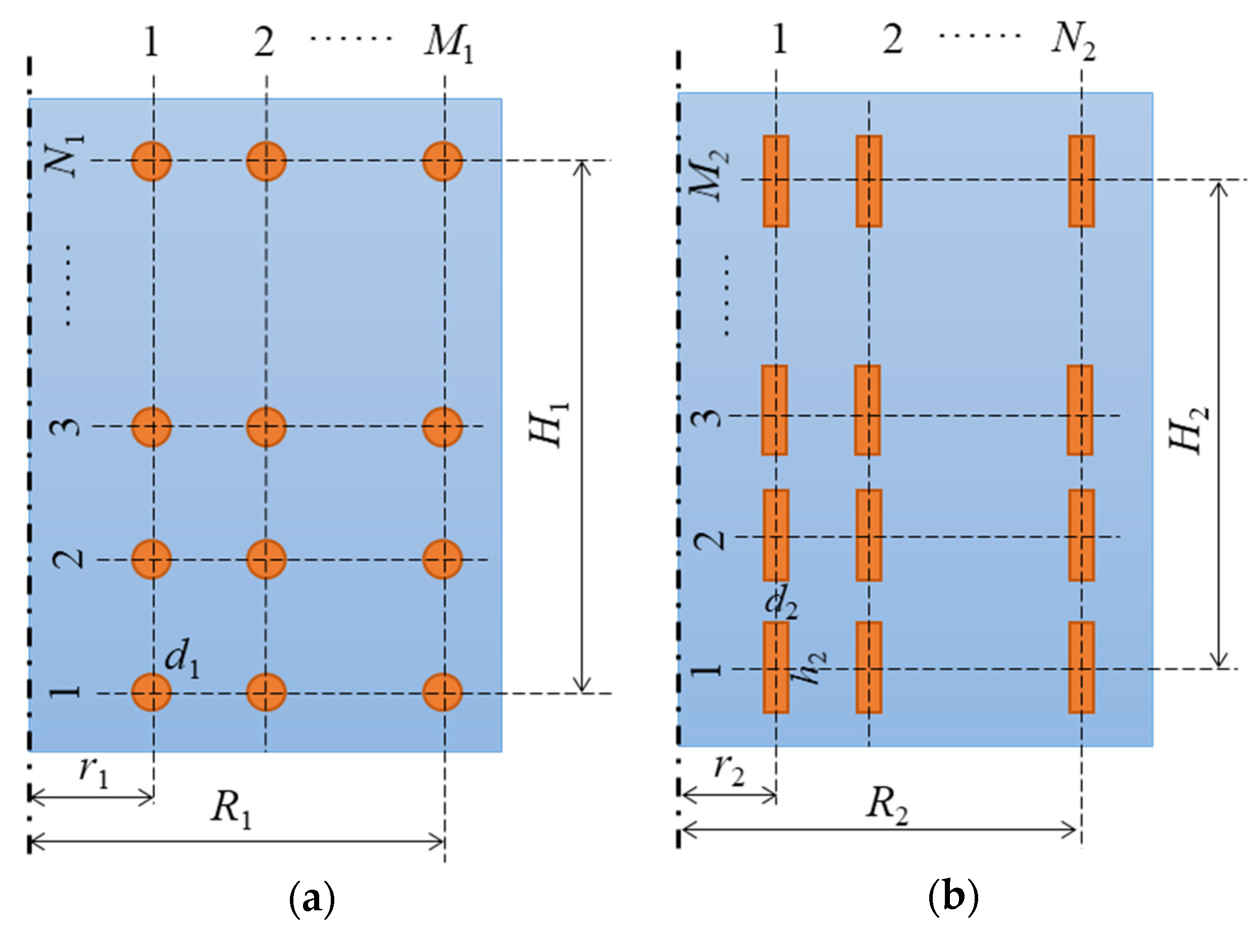
2.2. Parameterized Finite Element Modeling

Since the helical structures of both inductors have central symmetry, to improve the computational efficiency, the 2D axisymmetric models of the above two types of air-core inductors are established in COMSOL Multiphysics version 6.2. Due to the skin effect of the conductor, to improve the resolution of the electromagnetic field calculations for the conductor and the nearby air domain, the surface mesh of the conductor was stratified and refined. The mesh transitions from a dense grid in the conductor domain to a sparse grid in the far-field air domain, as shown in Figure 3. The conductor material is copper, with a conductivity of 5.998 × 10⁷ S/m.

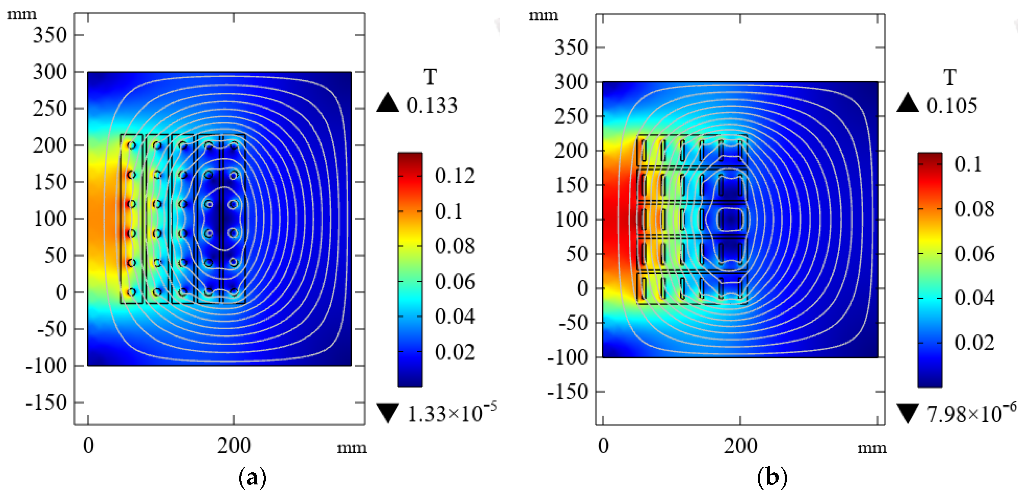
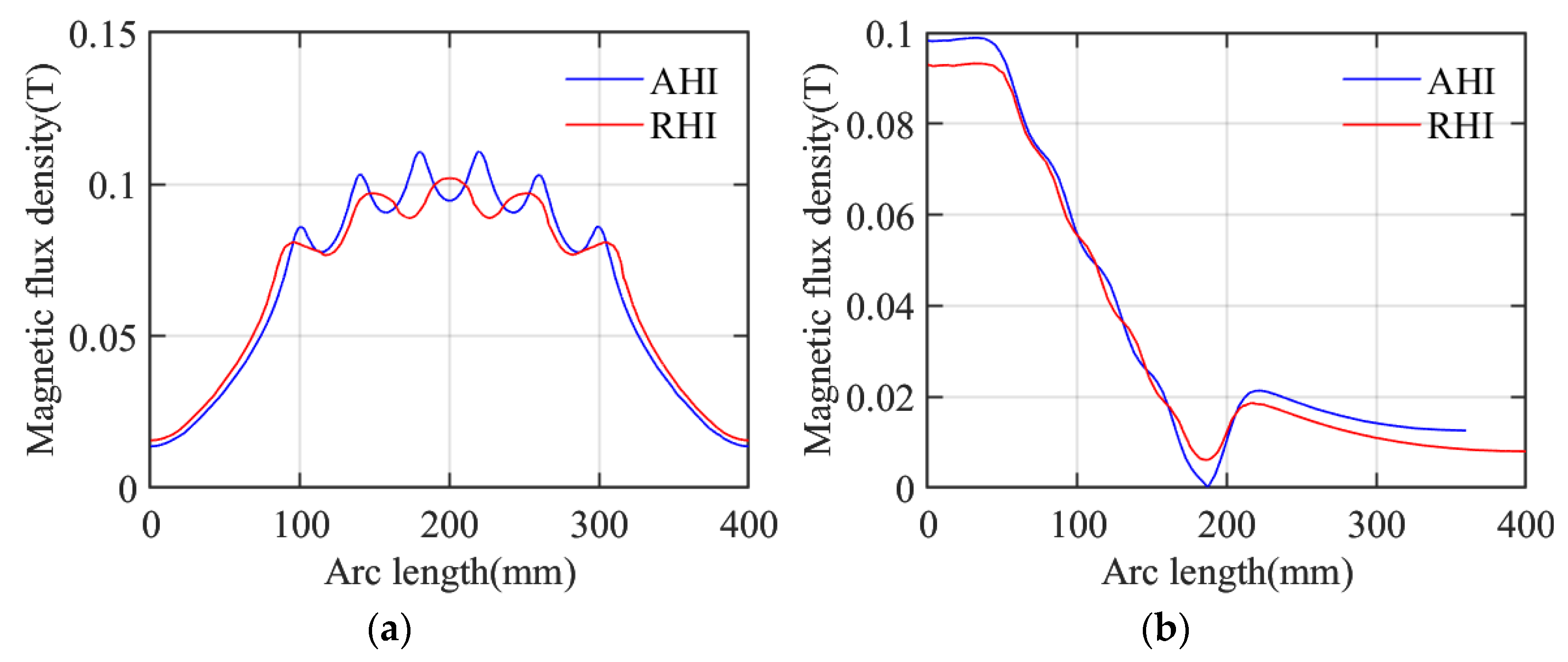
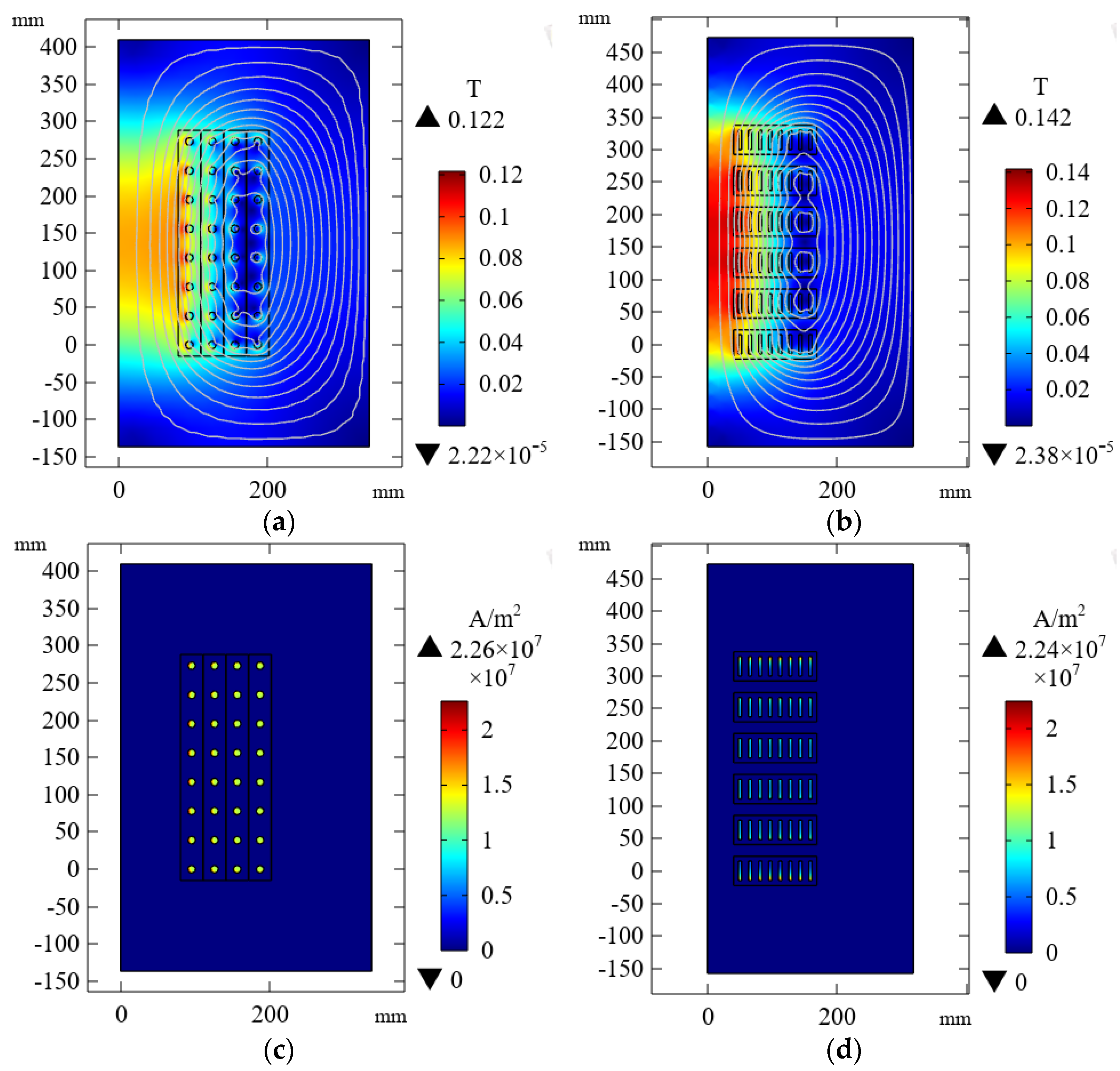
2.3. Spatial Magnetic Field Distribution Characteristics of Inductors

Figure 4 shows the distribution of magnetic flux density in space for the two types of inductors under the excitation of a current magnitude of 1000 A and a frequency of 100 Hz. The distribution patterns of the magnetic field in the space around the inductor coils are similar, with the magnetic flux density being more concentrated in the inner areas of the coils and gradually decreasing in the outer areas of the coils. The peak value of the magnetic flux density appears near the surface of the innermost conductor, close to the center of the coil.

To quantitatively analyze the spatial distribution of magnetic flux density in the two types of inductors, cross-sectional lines were taken along the central axial and radial directions of the inductor windings, and the variation curves of magnetic flux density along these paths were obtained, as shown in Figure 5. The magnetic flux density of the two types of inductors is symmetrically distributed along the axis of the coil and exhibits a periodic pattern of alternating peaks and valleys; that is, peak values appear at the corresponding positions of the conductors, and valley values appear between adjacent conductors. The variation law of magnetic flux density along the radial direction of the windings is as follows: a peak appears on the inner side of the windings, and then it gradually decreases from the inside to the outside of the windings until it approaches zero at the center of the magnetic flux contour lines. After that, a small peak appears on the outer side of the windings, followed by a gradual decrease towards the far-field air domain.

3. Generation of Training Data and Modeling of BP Neural Network

3.1. Monte Carlo Sampling

The design variables for the AHI inductor include the inner winding radius r₁, outer winding radius R₁, axial number of turns N₁, radial number of layers M₁, and inductor height H₁. The design variables for the RHI inductor include the inner winding radius r₂, outer winding radius R₂, radial number of turns N₂, axial number of layers M₂, and inductor height H₂. The value ranges of each design variable are shown in

Table 1. Range of design variables for both types of inductors.

Inductor Type	Structural Design Variables	Lower Design Limit	Upper Design Limit
AHI	r1 (mm)	50	100
	R1 (mm)	150	250
	N1	5	14
	M1	3	7
	H1 (mm)	200	400
RHI	r2 (mm)	50	100
	R2 (mm)	150	250
	N2	5	14
	M2	5	9
	H2 (mm)	200	400

.

To ensure the quality of automatic mesh generation during parametric finite element analysis, certain spatial constraints need to be satisfied between the design variables. Additionally, the number of coil turns and layers should be rounded to integers. In summary, the constraint conditions for the design variables are as follows:

$$\{\begin{array}{l}3(N_1-1)d_1\le H_1\\ 3(M_1-1)d_1\le R_1-r_1\\ 1.5(M_2-1)h_2\le H_2\\ 3(N_2-1)d_2\le R_2-r_2\\ N_1,M_1,N_2,M_2\in N^{*}\end{array},$$

(1)

In the formula, d₁ = 10 mm, d₂ = 5 mm, and h₂ = 30 mm are all constants.

For the relatively complex constraint conditions mentioned above, the conventional Latin Hypercube method is difficult to effectively perform sampling. In comparison, using the Monte Carlo method for sampling is a more appropriate choice. Monte Carlo is a random sampling method that can randomly draw samples from a defined probability distribution to estimate overall parameters or characteristics [20]. As the number of trials increases, this estimated value approaches the true probability value. This method is not restricted by the specific form of the problem and has broad applicability.

The optimization objective of this paper is to find the optimal structural parameters when the current distribution non-uniformity coefficient W_j is minimized under the condition that the volumetric inductance density L/V meets certain criteria. The spatial volumes occupied by the AHI inductor and the RHI inductor are respectively:

$$V_1=\pi {(R_1+0.5d_1)}^2(H_1+d_1),$$

(2)

$$V_2=\pi {(R_2+0.5d_2)}^2(H_2+h_2),$$

(3)

The non-uniformity coefficient of the current distribution within the winding is defined as follows:

$$W_j={\displaystyle \frac{j_{\max }}{j_{ave}}}={\displaystyle \frac{j_{\max }}{\frac{{\displaystyle ∯jdA}}{A}}},$$

(4)

where j is the current density in the cross-section, j_max is the maximum current density, j_ave is the average current density, and A is the cross-sectional area of the winding. A smaller value of W_j indicates a more uniform current distribution in the cross-section.

Within the value ranges of each design variable, the Monte Carlo sampling method was used to draw 100 sets of sample points for both the AHI inductor and the RHI inductor. Then, through parameterized finite element analysis of the inductor’s electromagnetic field, the training dataset was obtained.

3.2. Modeling of BP Neural Network

BP neural network is a feed-forward neural network trained by a backpropagation algorithm. It consists of an input layer, hidden layers, and an output layer, capable of learning and storing a large number of input-output pattern mapping relationships [21]. In this paper, a single-hidden-layer BP neural network is used, and the training function utilizes the ‘trainlm’ function. The structural parameters of the AHI inductor and the RHI inductor are taken as the input parameters of the neural network, while the inductance value L, the volumetric inductance density L/V, and the current distribution non-uniformity coefficient W_j are used as the output parameters. The prediction accuracy of a neural network is influenced by the number of hidden layer units, which has a direct relationship with the number of input and output parameters. The calculation formula is as follows:

$$K=\sqrt{k+m}+c,$$

(5)

where K is the number of hidden layer units, k is the number of input parameters, m is the number of output parameters, and c is a constant value between 1 and 10.

After experimenting with different values for training parameters, it was found that when the number of hidden layer units in the AHI is set to 7, the neural network training results in the smallest error. For the RHI, the smallest training error is achieved when the number of hidden layer units is set to 8. From the aforementioned 100 sets of sample data for each, 70 sets were selected as the training set, with the remaining 30 sets serving as the test set. After training the neural network with the training set, the relationship between the output parameters and the input parameters of the neural network model was obtained, as shown in Figure 6. The errors between the predicted values and the real values of each output parameter are relatively small.

To evaluate the accuracy of the BP neural network fitting model, the coefficient of determination R² and the Relative Root Mean Square Error (RRMSE) are used as evaluation metrics. The calculation formulas for these two metrics are as follows

$$R^2={\displaystyle \frac{{\displaystyle \sum {({\widehat{y}}_i-\overline{y})}^2}}{{\displaystyle \sum {(y_i-\overline{y})}^2}}},$$

(6)

$$RRMSE={\displaystyle \frac{\sqrt{{\displaystyle \sum {({\widehat{y}}_i-\overline{y})}^2}}}{\overline{y}\times m_1}},$$

(7)

In the formulas, ŷ represents the predicted value, ȳ represents the average value, y represents the true value, and m₁ represents the number of samples. A higher R² value closer to 1 indicates a better fitting accuracy of the model. A lower RRMSE value closer to 0 suggests a smaller fitting deviation and more reliable accuracy of the model.

The R² and RRMSE values for both AHI and RHI inductors based on the fitting results of the BP neural network are listed in

Table 2. R² and RRMSE values for both types of inductors with different output parameters.

Inductor Type		Evaluation Index	L	L/V	Wj
AHI	Training samples	R2	0.9987	0.9985	0.9992
		RRMSE	0.0033	0.0027	0.0006
	Testing samples	R2	0.9963	0.9965	0.9984
		RRMSE	0.0078	0.0063	0.0011
RHI	Training samples	R2	0.9982	0.9984	0.9990
		RRMSE	0.0037	0.0026	0.0005
	Testing samples	R2	0.9903	0.9938	0.9960
		RRMSE	0.0092	0.0055	0.0013

. The data in the table show high fitting accuracy for both the training set and the testing set, indicating that the training effect of the BP neural network model is good.

4. Analysis of Factors Affecting the Inductance Value of Inductors

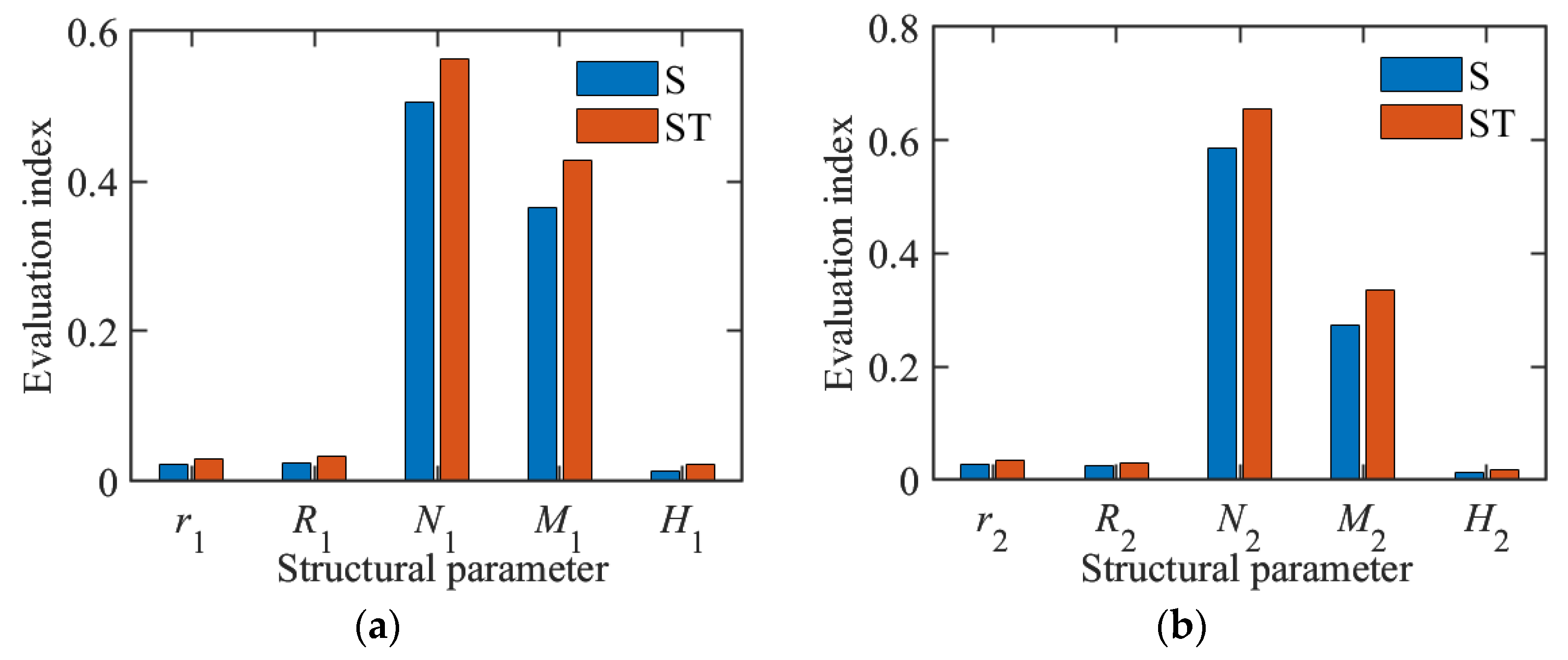
4.1. Sensitivity Analysis of Structural Parameters

Before proceeding with the optimization design, this paper first conducts a sensitivity analysis to investigate the degree of impact of changes in various structural parameters of the inductor on its inductance value. It is assumed that there exists a mathematical mapping relationship between the inductance value of the inductor and its structural parameters, which can be expressed as

$$L=f(X),$$

(8)

where L represents the inductance value of the inductor, and X = (X₁, X₂, …, X_i) represents the vector composed of various structural parameters of the inductor.

Variance analysis methods are employed to evaluate the sensitivity of the structural parameters to the inductance value, thereby assessing their importance. Sobol’s indices are commonly used variance analysis metrics, which are divided into the first-order effect index S_i and the total effect index S_Ti. The first-order effect index S_i represents the contribution of the variance of each input variable to the variance of the dependent variable, thus quantifying the sensitivity of a single variable to the model.

$$S_i={\displaystyle \frac{V_i}{V(L)}},$$

(9)

In the formula, V_i represents the variance contribution of the main effect of variable X_i, and V(L) represents the total variance of the mathematical model. The total effect index S_Ti reflects the combined influence of the variance of each input variable, along with its interactions with other input variables, on the variance of the dependent variable. It provides a more comprehensive understanding of the impact of the complex relationships between various input variables on the model output.

$$S_{Ti}={\displaystyle \frac{V_i+{\displaystyle {\sum }_{i\ne j}}{V}_{ij}+\dots +V_{1,2,\dots ,i,\dots ,k}}{V(L)}},$$

(10)

where V_ij is the variance contribution of the interaction effect of variables X_i and X_j, and so on.

Sobol analysis is a commonly used method for sensitivity analysis, which is based on using variance to characterize the uncertainty of the output. In this paper, based on the trained BP neural network fitting model mentioned earlier, Monte Carlo sampling was performed in the design space with 4000 sampling points, and Sobol indices were calculated for them. The results are shown in Figure 7. Within the designed variable range, for the AHI inductor, the axial number of turns N₁ has the greatest influence on its inductance value, followed by the radial number of layers M₁, while the other parameters have relatively smaller impacts. For the RHI inductor, the radial number of turns N₂ has the greatest influence on its inductance value, followed by the axial number of layers M₂.

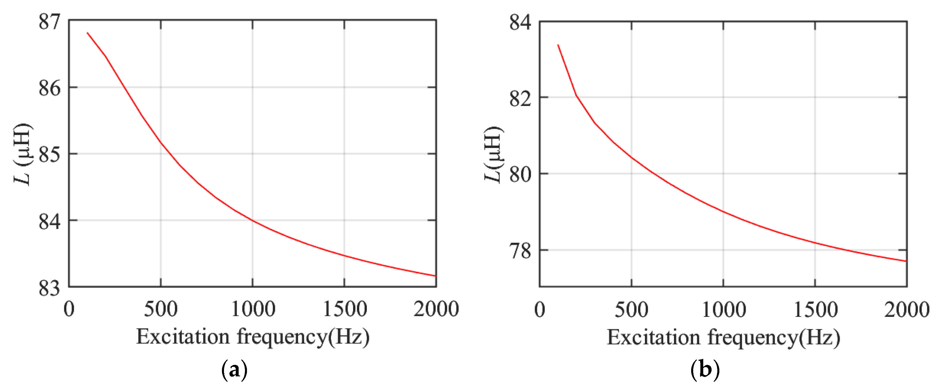
4.2. The Effect of Excitation Frequency

To explore the impact of different excitation frequencies on the inductance value of inductors, both types of inductors were subjected to an incremental approach, where the excitation frequency was increased by 100 Hz at a time, gradually increasing it up to 2000 Hz. Figure 8 shows the variation curves of the inductance values for the two types of inductors at different frequencies. As the excitation frequency increases, the inductance value of the inductors gradually decreases.

Figure 9 shows the magnetic flux density distribution cloud chart of the two types of inductors under 500 Hz and 2000 Hz excitation. It can be seen that the overall spatial distribution pattern of magnetic flux density is basically consistent with the aforementioned, but what differs is that with the increase in excitation frequency, the peak value of the inductor’s magnetic flux density gradually increases, and the distribution of magnetic field strength in space becomes more uneven.

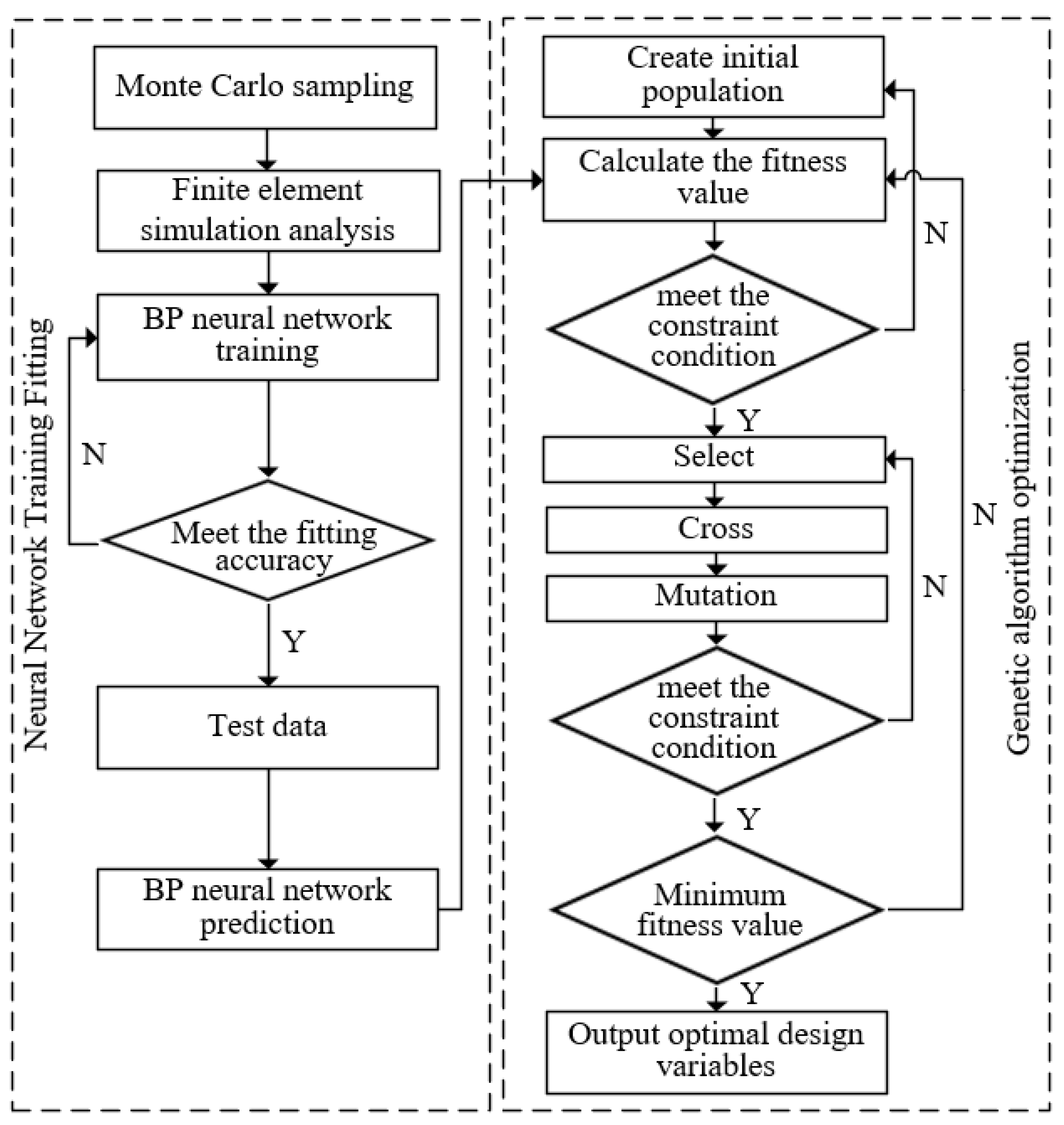
5. Optimization of Inductor Structural Parameters Based on BP-GA Algorithm

5.1. Mathematical Model for the Structural Optimization of Inductors

The mathematical model for the structural optimization of inductors encompasses three components: optimization objectives, design variables, and constraints. The optimization objective is the current distribution non-uniformity coefficient W_j in the inductor. A smaller W_j can effectively reduce the problem of thermal stress concentration caused by uneven current distribution during inductor operation. The design variables are the structural parameters of the inductor. The constraints include the value range of the inductor design variables and its volumetric inductance density, L/V. Due to the mutual influence and constraints between factors such as inductance and current density, the structural design becomes complex. In order to ensure the compactness of the structure and improve the energy storage density of the pulsed power supply, the volumetric inductance density L/V was introduced as an additional constraint [22]. A higher L/V implies that a higher inductance value can be achieved within a limited space. In this paper, the volumetric inductance density constraints for the two types of inductors are referenced to the average volumetric inductance density of their respective 100 sets of sample data, which are 3500 μH/m³ and 4500 μH/m³. The established optimization models for the AHI and RHI inductors are as follows:

$$\{\begin{array}{l}\min W_j\\ {\displaystyle \frac{L}{V}}\ge 3500\mu {\mathrm{H}/\mathrm{m}}^3\\ X_{\min }\le X\le X_{\max }\\ 3(N_1-1){\mathrm{d}}_1\le H_1\\ 3(M_1-1)d_1\le R_1-r_1\\ N_1,M_1\in N^{*}\end{array},$$

(11)

$$\{\begin{array}{l}\min W_j\\ {\displaystyle \frac{L}{V}}\ge 4500\mu {\mathrm{H}/\mathrm{m}}^3\\ X_{\min }\le X\le X_{\max }\\ 1.5(M_2-1)h_2\le H_2\\ 3(N_2-1)d_2\le R_2-r_2\\ N_2,M_2\in N^{*}\end{array}$$

(12)

In the formula, W_j represents the current distribution non-uniformity coefficient, L/V represents the volumetric inductance density, and X_min and X_max are the value ranges of the design variables. N₁, M₁, H₁, r₁, and R₁ are the five design variables of the AHI inductor, while N₂, M₂, H₂, r₂, and R₂ are the five design variables of the RHI inductor. d₁ is the conductor diameter, d₂ is the conductor thickness, and h₂ is the height of a single turn, all of which are constants.

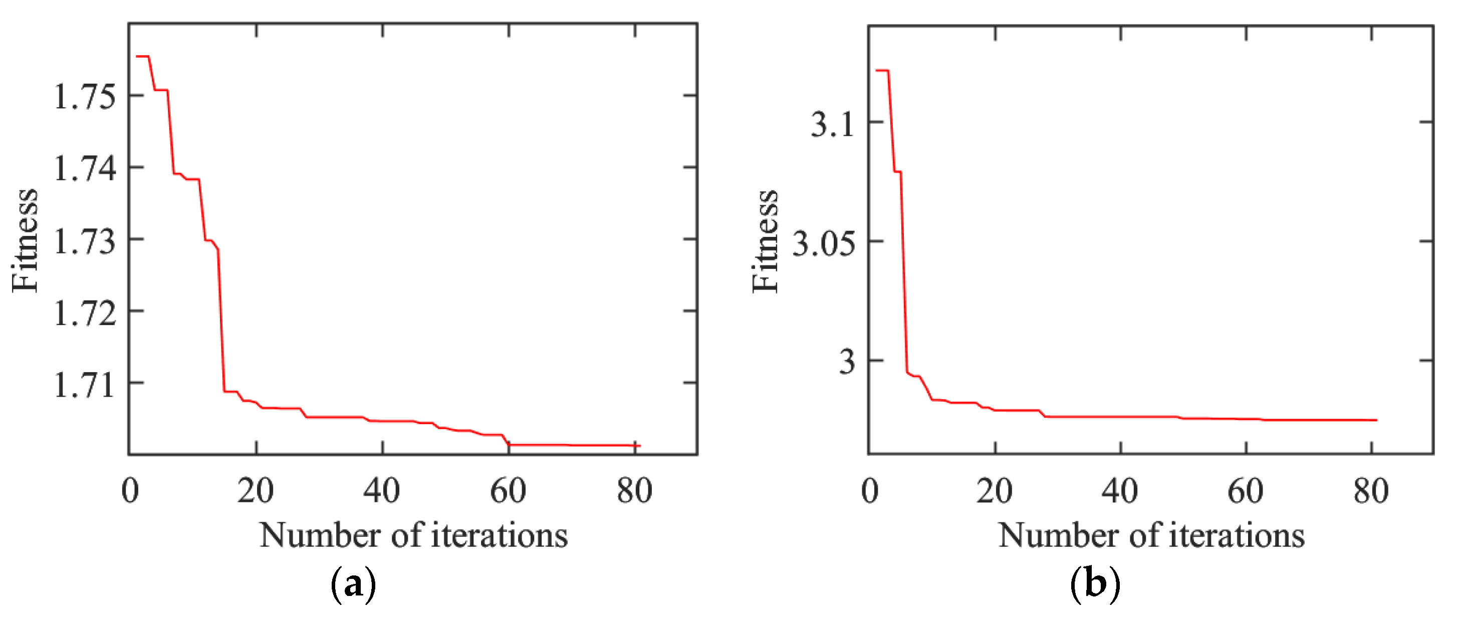
5.2. Optimization by BP-GA Joint Algorithm

A genetic algorithm (GA) is a search algorithm that simulates the mechanisms of natural selection and genetics in biological evolution. Encoding represents the possible solutions to a problem as chromosomes and gradually seeks the optimal solution through select, cross, and mutation operations, simulating the biological evolution process. The BP-GA algorithm combines the nonlinear mapping ability of a BP neural network with the fast optimization capability of genetic algorithms, and the complementary advantages of both make it more effective in solving complex optimization problems for inductor structural parameters.

The optimization objective of the inductor in this paper is to reduce the current distribution non-uniformity coefficient W_j. This is achieved by setting the fitness function value to W_j and then selecting the chromosome with the minimum fitness value to obtain the optimal result. Leveraging the previously trained BP neural network prediction model, the current distribution non-uniformity coefficient W_j is established as the individual fitness evaluation criterion in the genetic algorithm. Under this criterion, a lower fitness value indicates a better individual. Given that both input and output parameters are subject to strict constraints, after creating the initial population according to the constraints of the structural parameters in the genetic algorithm process, it is essential to ensure that the volumetric inductance density L/V of all individuals meets the constraints during the fitness value calculation. However, after the selection, crossover, and mutation operations, new individuals that do not satisfy the constraints may be generated. Therefore, it is necessary to re-examine newly generated individuals to ensure that they meet all constraints. The optimization process of the BP-GA joint algorithm is shown in Figure 10.

After optimization using the BP-GA joint algorithm, the optimal structural parameters of the air-core inductor were determined. As shown in Figure 11, for the AHI, after 60 iterations, the fitness value of the individuals tends to stabilize, with the best fitness value being 1.7013. For the RHI, its fitness value gradually converges after approximately 63 iterations, with the best fitness value being 2.9749.

The optimized structural dimensions of the two types of inductors after the optimization solution are shown in

Table 3. The structure parameters of two kinds of inductors after the BP-GA joint algorithm.

Inductor Type	Structural Design Variables	Optimal Parameter
AHI	r1 (mm)	95.15
	R1 (mm)	186.70
	N1	8
	M1	4
	H1 (mm)	272.89
RHI	r2 (mm)	50.34
	R2 (mm)	158.72
	N2	8
	M2	6
	H2 (mm)	315.03

. The optimal dimensions for the AHI are: coil inner diameter 95.15 mm, coil outer diameter 186.70 mm, axial turns 8, radial layers 4, inductance height 272.89 mm, and the inductor inductance value is 114.66μH. The optimal dimensions for the RHI are: coil inner diameter 50.34 mm, coil outer diameter 158.72 mm, radial turns 8, axial layers 6, inductance height 315.03 mm, and the inductor inductance value is 127.88 μH.

5.3. Finite Element Validation

To verify the rationality of the inductor structural parameters obtained through optimization using the BP-GA joint algorithm, a finite element analysis model of the inductor’s electromagnetic field was re-established based on the optimized dimensions. Figure 12 shows the magnetic flux density and current density distributions of the two optimized inductors under the excitation of a current magnitude of 1000 A and frequency of 100 Hz.

After data processing, the finite element calculation results after optimization were compared in detail with the training sample data, as shown in the relevant statistical data in

Table 4. Finite element analysis data comparison before and after optimization of the two inductors.

Inductor Type		L (μH)	L/V (μH/m3)	Wj
AHI	Sample of optimal L/V	486.0346	8459.9692	2.8657
	Sample of optimal Wj	116.7442	3531.5769	1.7934
	post-optimization	114.6565	3510.6846	1.7115
RHI	Sample of optimal L/V	803.1687	13330.8319	3.9640
	Sample of optimal Wj	114.9423	4591.9504	3.0388
	post-optimization	127.8841	4539.2142	2.8768

.

When the AHI is at its optimal dimensions, the current distribution non-uniformity coefficient W_j is 1.7115, which is a reduction of 40.28% compared to the sample with the best volumetric inductance density L/V in the sampling, and a reduction of 4.57% compared to the optimal sample that also meets the constraint of a volumetric inductance density L/V greater than 3500 μH/m³ in the sampling. The error between the finite element verified calculation results and the prediction results of the BP neural network model is only 0.60%.

When the RHI is at its optimal dimensions, the current distribution non-uniformity coefficient W_j is 2.8768, which is a reduction of 27.43% compared to the sample with the best volumetric inductance density L/V in the sampling. It is also a reduction of 5.33% compared to the optimal sample that meets the constraint of a volumetric inductance density L/V greater than 4500 μH/m³ in the sampling. The error between the finite element verified calculation results and the prediction results of the BP neural network model is 2.46%.

From the above, it can be seen that the inductor design parameters obtained after optimization using the BP-GA joint algorithm, when compared with the optimal data in the training samples, have all reduced the current distribution non-uniformity coefficient W_j, meaning that the uniformity of the inductor’s current distribution has been improved. In addition, the optimized inductor parameters were further validated by finite element simulation, which confirmed the high predictive accuracy of the constructed BP neural network model, with the prediction error of the current distribution non-uniformity coefficient W_j for both types of inductors being within 3%.

6. Conclusions

In this paper, the combination of the powerful nonlinear mapping capability of the BP neural network and the search capability of the genetic algorithm is used for the structural optimization of axial and radial helical multi-winding inductors, achieving good results. The main work and conclusions are as follows:

(1) Based on Monte Carlo sampling and parametric finite element simulations of AHI and RHI inductors, training and testing datasets for neural networks were generated. Nonlinear mapping models between the inductor’s volumetric inductance density L/V, current distribution non-uniformity coefficient W_j, and inductor structural parameters were established through BP neural networks. On this basis, the current distribution non-uniformity coefficient was used as the fitness function of the genetic algorithm, and the volumetric inductance density was used as a constraint. The optimal combination of inductor structural parameters was obtained through rapid optimization processes, such as selection, crossover, and mutation.

(2) The Sobol index was calculated to analyze the sensitivity of the inductor’s inductance value to changes in the structural parameters. For the AHI, the axial turns N₁ have the greatest impact on the inductance value, followed by the radial layers M₁. For the RHI, the inductance value is most significantly affected by the radial turns N₂, followed by the axial layers M₂. At the same inductance value, the RHI has a higher volumetric inductance density and a more compact structure than the AHI.

(3) After joint optimization using the BP-GA algorithm, the current distribution non-uniformity coefficient W_j of the AHI was reduced by 40.28% compared to the sample with the optimal volumetric inductance density L/V in the sampling and reduced by 4.57% compared to the sample with the best W_j in the sampling. The current distribution non-uniformity coefficient W_j of the RHI was reduced by 27.43% compared to the sample with the optimal volumetric inductance density L/V in the sampling and reduced by 5.33% compared to the sample with the best W_j in the sampling. Further verification using finite element analysis showed an error within 3%, demonstrating the practicality of the BP-GA joint algorithm in inductor structural optimization.

References

1. Tian, M.; Wang, T.; Zhang, H.; Yi, L. Review and prospect of controllable inductors. J. Jilin Univ. Eng. Technol. Ed. 2023, 53, 328–345. [Google Scholar]
2. Zhang, Y.; Zhao, J.; Qin, C.; Zhang, R.; Li, S. Analysis of turn-to-turn short circuit magnetic field of dry-type air-core inductor. In Proceedings of the 2023 3rd New Energy and Energy Storage System Control Summit Forum (NEESSC), Mianyang, China, 26–28 September 2023. [Google Scholar]
3. Bai, G.; Gu, C.; Lai, L. Electromagnetic analysis of an air-core HTS transformer. IEEE Trans. Appl. Supercond. 2019, 29, 1–3. [Google Scholar] [CrossRef]
4. Jin, L.; Zhu, D.; Yang, Q.; Zhang, J.; Gong, D. Grey-box model and optimization for inductance calculation of EHV inductors. Trans. China Electrotech. Soc. 2022, 37, 6093–6103. [Google Scholar]
5. Wang, T.; Tian, M.; Zhang, H.; Zhang, Y. Unified study on electromagnetic characteristics of controllable inductors based on transformer models. Power Syst. Technol. 2023, 47, 2947–2956. [Google Scholar]
6. Yuan, F.; Lv, K.; Liu, J.; Zhou, B.; Tang, B. Optimization method for coil structure of iron-core inductors based on electromagnetic-thermal-structural multi-physics coupling. Trans. China Electrotech. Soc. 2022, 37, 6431–6441. [Google Scholar]
7. Hao, S.; Li, Z.; Ma, F.; Li, B. Characteristic analysis of inductor in pulsed power supply changing with shape ratio. In Proceedings of the 2020 Spring International Conference on Defence Technology (ICDT Spring), Nanjing, China, 20–24 April 2020. [Google Scholar]
8. Liu, X.; Yu, X.; Li, Z. Inductance calculation and energy density optimization of the tightly coupled inductors used in inductive pulsed power supplies. IEEE Trans. Plasma Sci. 2017, 45, 1026–1031. [Google Scholar] [CrossRef]
9. Jiang, Z.; Zhou, H.; Song, J.; Yu, Y.; Weng, X. Calculation and experimental analysis of temperature field in dry-type air-core inductor. Trans. China Electrotech. Soc. 2017, 32, 218–224. [Google Scholar]
10. Shetty, C.; Kandeel, Y.; Ye, L.; O’Driscoll, S.; McCloskey, p.; Duffy, M.; Mathúna, C.Ó. Analytical expressions for inductances of 3-D air-core inductors for integrated power supply. IEEE J. Emerg. Sel. Top. Power Electron. 2022, 10, 1363–1383. [Google Scholar] [CrossRef]
11. Liu, Z.; Wang, J.; Geng, Y.; Shi, C. Calculation and analysis of magnetic field and inductance of dry-type air-core inductor. High Volt. Appar. 2003, 39, 7–11. [Google Scholar]
12. Gan, Y.; Bai, R.; Zhang, Q. Steady-state electromagnetic field and electromotive force analysis of dry-type air-core inductor based on field-circuit coupling. Power Syst. Prot. Control. 2019, 47, 144–149. [Google Scholar]
13. Lin, Q. Magnetic field analysis of dry-type air-core inductor. Transformer 2019, 56, 29–33. [Google Scholar]
14. Ye, C.; Yu, K.; Zhang, G.; Pan, Y. The windings inductance calculation of an air-core compulsator. IEEE Trans. Magn. 2009, 45, 522–524. [Google Scholar]
15. Tan, W.; Zhou, L.; Gong, X.; Wu, W.; Ou, Q. Research on structural optimization design of controllable inductor with taps. Transformer 2019, 56, 9–14. [Google Scholar]
16. Li, S.; Lu, J.; Cheng, L.; Zhu, B. Stress analysis and structural design of pulsed inductor for electromagnetic launch. J. Natl. Univ. Def. Technol. 2019, 41, 39–45. [Google Scholar]
17. Sun, H.; Yu, X.; Li, Z.; Li, B.; He, H. Inductance calculation and structural optimization of toroidal circular disk-type inductors in IPPS. IEEE Trans. Plasma Sci. 2021, 49, 2247–2255. [Google Scholar] [CrossRef]
18. Li, Z.; Yu, X.; Ma, S.; Sha, Y. Structural parameter optimization of inductors used in inductive pulse power supply. IEEE Trans. Plasma Sci. 2015, 43, 1456–1461. [Google Scholar]
19. Li, Y.; Zhang, Z.; Zhu, L.; Jiang, M. Calculation and Design of Dry-Type Hollow Inductors. Transformer 2013, 50, 1–6. [Google Scholar]
20. Hung, Y.C. A review of Monte Carlo and quasi-Monte Carlo sampling techniques. Wiley Interdiscip. Rev. Comput. Stat. 2023, 16, e1637. [Google Scholar] [CrossRef]
21. Qi, S.; Lu, X.; Liu, H.; Zhu, L.; Wang, F. Application of BP Neural Network Optimized by Genetic Algorithm in Fault Diagnosis of Distribution Network. Electr. Power Sci. Technol. 2023, 38, 182–187. [Google Scholar]
22. Wang, Y.; Liu, L.; Zhang, M.; Zhang, W.; Li, P. Review of Turn-to-Turn Insulation Detection for Dry-Tors. Electr. Power Capacit. React. Power Compens. 2018, 39, 91–95. [Google Scholar]
Figure 1. 3D models of two types of inductors: (a) AHI and (b) RHI.
Electronics 13 03463 g001
Figure 2. Structural parameters of two types of inductors: (a) AHI and (b) RHI.
Electronics 13 03463 g002
Figure 3. Finite element mesh: (a) AHI and (b) RHI.
Electronics 13 03463 g003
Figure 4. Spatial distribution of magnetic flux density around inductors: (a) AHI and (b) RHI.
Electronics 13 03463 g004
Figure 5. Radial and axial variation of the flux density of inductors: (a) AHI and (b) RHI.
Electronics 13 03463 g005
Figure 6. BP neural network model training results for two types of inductors: (a) Inductance L of AHI (b) Inductance L of RHI (c) Volumetric inductance density L/V of AHI (d) Volumetric inductance density L/V of RHI (e) Current distribution non-uniformity coefficient Wj of AHI (f) Current distribution non-uniformity coefficient Wj of RHI.
Electronics 13 03463 g006
Figure 7. Sobol index of structural parameters for two types of inductors: (a) AHI and (b) RHI.
Electronics 13 03463 g007
Figure 8. Variation in inductance of inductor with excitation frequency: (a) AHI (b) RHI.
Electronics 13 03463 g008
Figure 9. Magnetic flux density distribution of inductors at 500 Hz and 2000 Hz frequencies: (a) AHI 500 Hz (b) AHI 2000 Hz (c) RHI 500 Hz (d) RHI 2000 Hz.
Electronics 13 03463 g009
Figure 10. The optimization process of the BP-GA joint algorithm.
Electronics 13 03463 g010
Figure 11. Fitness evolution curve: (a) AHI and (b) RHI.
Electronics 13 03463 g011
Figure 12. The optimized inductor finite element simulation results: (a) Magnetic flux density distribution of AHI (b) Magnetic flux density distribution of RHI (c) Current density distribution of AHI (d) Current density distribution of RHI.
Electronics 13 03463 g012