Online Joint Optimization of Virtual Network Function Deployment and Trajectory Planning for Virtualized Service Provision in Multiple-Unmanned-Aerial-Vehicle Mobile-Edge Networks

Abstract

The multiple-unmanned-aerial-vehicle (multi-UAV) mobile edge network is a promising networking paradigm that uses multiple resource-limited and trajectory-planned unmanned aerial vehicles (UAVs) as edge servers, upon which on-demand virtual network functions (VNFs) are deployed to provide low-delay virtualized network services for the requests of ground users (GUs), who often move randomly and have difficulty accessing the Internet. However, VNF deployment and UAV trajectory planning are both typical NP-complete problems, and the two operations have a strong coupling effect: they affect each other. Achieving optimal virtualized service provision (i.e., maximizing the number of accepted GU requests under a given period T while minimizing the energy consumption and the cost of accepting the requests in all UAVs) is a challenging issue. In this paper, we propose an improved online deep reinforcement learning (DRL) scheme to tackle this issue. First, we formulate the joint optimization of the two operations as a nonconvex mixed-integer nonlinear programming problem, which can be viewed as a sequence of one-frame joint VNF deployment and UAV-trajectory-planning optimization subproblems. Second, we propose an online DRL based on jointly optimizing discrete (VNF deployment) and continuous (UAV trajectory planning) actions to solve each subproblem, whose key idea is establishing and achieving the coupled influence of discrete and continuous actions. Finally, we evaluate the proposed scheme through extensive simulations, and the results demonstrate its effectiveness.

1. Introduction

The multiple-unmanned-aerial-vehicle (multi-UAV) mobile-edge network is a promising networking paradigm that uses multiple resource-limited unmanned aerial vehicles (UAVs) as edge servers to serve ground users (GUs) [1]. Because UAVs are low in cost and flexible and deliver a prompt response, multi-UAV mobile-edge networks can be applied in harsh environments where terrestrial mobile edge networks do not work well, such as (1) forest, mountain, and desert areas, where terrestrial mobile edge networks cannot be reliably established or cannot be established at all, and (2) disaster areas, where terrestrial mobile-edge networks are destroyed by natural disasters [1]. First, the UAV communication range is limited, and GUs may move randomly within a wide range. Second, GU requests occur in real time, so UAV trajectories should be planned to serve as many GUs as possible within the request delay requirement. Moreover, the services are provided by virtual network functions (VNFs), which are software instances mapping from dedicated network service hardware [2,3]. Compared with hardware, the cost of using VNFs is lower, and VNFs can be flexibly deployed online on UAVs to meet GUs’ real-time and changing service requests.

Although using UAVs and VNFs to serve GUs has many benefits, achieving the optimal virtualized service provision (i.e., maximizing the number of accepted GUs requests under a given period T while minimizing the energy consumption and the cost of accepting the requests in all UAVs) via VNF deployment and UAV trajectory planning is challenging for the following two reasons: (1) VNF deployment and UAV trajectory planning are both typical NP-complete problems and (2) the two operations have a strong coupling effect, meaning that they affect each other. Specifically, optimal UAV trajectory planning that consumes minimum energy may cause poor VNF deployment, which leads to increased computational resource occupation and/or frequently deployed VNF instance switching, leading to a high cost of accepting requests. Conversely, an optimal and low-cost VNF deployment decision that is achieved with low computation resource occupation and no VNF instance switching may lead to poor UAV trajectory planning with high energy consumption because UAVs fly with high-energy power velocity to accept target GU requests. Thus, to optimize virtualized service provision, the joint optimization of VNF deployment and UAV trajectory planning is both important and necessary.

Based on the above challenge, we studied the joint optimization of VNF deployment and UAV trajectory planning to maximize the number of accepted GU requests under a given period T while minimizing the energy consumption and the cost of accepting the requests for all UAVs, in which the cost is composed of the instantiation cost of deploying VNF instances and the computing cost of processing requests in the VNF instances. To achieve this, we first formulated the proposed joint optimization as a nonconvex mixed-integer nonlinear programming problem, which can be viewed as a sequence of one-frame joint VNF deployment and UAV trajectory planning optimization subproblems. Second, we obtained, from simple analysis, that (1) the problem can be further formulated as a Markov decision process, which can be solved using a deep reinforcement learning (DRL) scheme, and (2) VNF deployment decisions are limited (discrete), and UAV trajectory plannings are infinite (continuous). Finally, we developed an improved online DRL based on jointly optimizing discrete (VNF deployment) and continuous (UAV trajectory planning) actions to solve the proposed problem by solving each subproblem.

The key idea of the proposed online DRL is establishing and achieving the coupled influence of discrete and continuous actions, which is achieved using two key designs. The first is the neural network design, which establishes the coupled relationship between discrete and continuous actions, with two neural networks used to obtain discrete and continuous actions, which are named Online-VNF-Qnetwork and UAVs-Trajectories Actor Network, respectively. Because the input of the neural network affects the output, continuous action is taken as one part of Online-VNF-Qnetwork’s input to obtain discrete action; similarly, discrete action is one part of the UAVs-Trajectories’ Actor Network’s input to obtain continuous action. The second is the training process designed for online joint optimization by learning the coupling relationship. To learn the influence of continuous action on discrete action, the sum of the reward obtained by discrete action and the reward obtained by continuous action (which is influenced by the discrete action) is used as Online-VNF-Qnetwork’s reward to fine-tune the discrete action, so Online-VNF-Qnetwork can determine the VNF deployment, optimizing the whole joint operation. To learn the influence of discrete action on continuous action, the approximate UAV flight areas are determined using the current VNF deployment. The reward used to adjust continuous action is jointly determined by the continuous action and discrete action related to it.

The main contributions of this study are as follows.

• We studied joint VNF deployment and UAV trajectory planning optimization in multi-UAV mobile-edge networks with the aim of maximizing the number of accepted GU requests under a given period T while minimizing both the energy consumption and the cost of accepting the requests for all UAVs with the constraints on their resources and the latency requirement of real-time requests. To the best of our knowledge, we are the first to jointly optimize VNF deployment and UAV trajectory planning based on emphasizing the coupling effect of the two processes to maximize the accepted number of requests under a given period T while minimizing both energy consumption and the cost, where the number of accepted requests is related to two process decisions, energy consumption is decided by UAV trajectories, and the cost is mainly related to VNF deployment.
• We formulated the proposed online joint problem as a nonconvex mixed integer nonlinear programming problem, and we designed an online DRL based on jointly optimizing discrete and continuous actions. The proposed algorithm can be used to solve real-time online joint problems of discrete and continuous variables that are coupled.
• We performed numerous simulations to verify algorithm performance. We compared the proposed algorithm with some baseline algorithms through simulations to verify that our algorithm is promising.

The rest of this paper is organized as follows: In Section 2, we review the related studies. Section 3 describes the system model and the formulated problem. In Section 4, we propose an online DRL based on jointly optimizing discrete and continuous actions. Section 5 describes the evaluation of the performance of the proposed algorithm, and Section 6 outlines our conclusions.

2. Related Studies

In this section, we review three kinds of related studies.

2.1. VNF Deployment in Mobile-Edge Networks with Terrestrial Fixed-Edge Servers

This area has been heavily investigated. P. T. A. Quang et al. [4] discussed service deployment in mobile networks. When placing a service on several noncooperative domains, they considered how to deploy services with the allocation of a virtual network function–forwarding graph (VNF-FG) so that the quality of service could be fulfilled. Thus, they developed a deep-reinforcement-learning-based VNF-FG-embedding approach. Z. Xu et al. [5] discussed the placement of Internet of Things (IoT) applications and their corresponding VNFs. For when IoT applications and their VNFs need to be placed in the same location, they devised an exact solution, an approximation algorithm, and a heuristic algorithm. When IoT applications and their VNFs are deployed in different locations, they designed a heuristic algorithm. Y. Ma et al. [6] investigated VNF provision in mobile-edge computing (MEC) networks with consideration of user mobility and service delay requirements. They proposed a constant approximation algorithm to solve the utility-maximization problem and designed an online algorithm for the accumulative throughput-maximization problem. Other researchers [7] aimed to maximize user request admissions while minimizing their admission cost. For times when the resources are sufficient to accept all requests, they proposed an integer linear programming (ILP) solution and two efficient heuristic algorithms to solve the cost minimization problem. For times when resources are limited, an ILP solution was designed for small problems and an efficient algorithm for large problems. H. Ren et al. [8] discussed the NFV-enabled multicasting problem in MEC networks. For a single multicast request admission, they designed an approximation algorithm without delay consideration and a heuristic with delay consideration. For a set of multicast requests, they developed a heuristic to maximize the system throughput while minimizing the implementation cost. M. Huang et al. [9] considered reliability-aware VNF instances’ provisioning in MEC networks and aimed to maximize the network throughput. They developed an approximation algorithm to solve the problem. Additionally, they proposed a constant approximation algorithm to solve the problem, assuming that only one primary and one secondary VNF instance are needed, and a dynamic programming algorithm for the problem assuming different VNF instances needed the same computing resources. S. Yang et al. [10] studied the minimization of the maximum link load ratio with the guarantee of each user’s requested delay. They proposed a randomized rounding approximation algorithm as the solution. Y. Qiu et al. [11] studied the VNF sharing and backup deployment problem in MEC servers, and their goal was to make the service function chains’ (SFCs’) actual reliabilities higher than the demand, while maximizing receiving request throughput and minimizing receiving cost. An online approximation solution was proposed to solve the problem. J. Li et al. [12] discussed how to maximize accumulative user satisfaction when providing VNFs in MEC networks, and they constructed an approximation algorithm to solve the problem. Additionally, researchers [13] investigated digital-twin-assisted, SFC-enabled, reliable service provisioning in MEC networks by exploiting the dynamics of VNF instance placement reliability. They proposed an ILP solution to solve the dynamic service admission maximization problem in the offline case and an approximation algorithm to solve the online service-cost-minimization problem. W. Liang et al. [14] investigated the service reliability augmentation problem in MEC networks, and they proposed an ILP solution and a randomized algorithm with certain resource violations to solve the problem. A deterministic heuristic algorithm without any resource violation was designed as the solution. F. Tian et al. [15] studied the joint optimization problem of VNF parallelization and deployment because the two steps affect each other. In small networks, an ILP method was proposed as the solution. For large networks, they proposed a solution by cascading I-SFG construction and VNF deployment approximation. J. Liang et al. [16] solved the problem regarding how to place VNFs on edge nodes in mobile-edge industrial Internet of Things to minimize the overall access delay by designing an online algorithm based on the heuristic algorithm. X. Wang et al. [17] discussed how to jointly optimize partial offloading and SFC mapping in an MEC system so that the long-term average cost is minimized, and they designed a cooperative dual-agent deep reinforcement learning algorithm to solve the problem.

These studies discuss VNF deployment problems in terrestrial mobile-edge networks with fixed-edge servers, so they focus on deployment only, even thogh some studies considered joint optimization. However, unlike these studies using fixed location terrestrial servers, we considered UAV mobility, so we then needed to consider the coupling effect between UAV trajectory planning and VNF deployment to jointly optimize the two processes.

2.2. VNF Deployment on Mobile-Edge Networks with Movable-Edge Servers

J. Bai et al. [18] explored the service-chain resilience in UAV-enabled MEC networks in terms of availability and reliability, and they presented a quantitative modeling approach based on a semi-Markov process. They focused on deploying VNFs in UAV networks so that service effectiveness could be increased. Their study provided guidance on UAV placement/trajectory optimization, which they did not study further. In our study, UAV trajectory planning needed to be optimized because this important online joint-optimization part achieves the goal. P. Zhang et al. [19] designed a DRL-assisted SFC embedding algorithm to more flexibly and efficiently provide user positioning services in collaborative cloud–edge–vehicle networks. In their study, the trajectories of vehicles used as movable-edge servers were not part of the solution: they were just a factor that needed to be considered when obtaining the VNF deployment solution. Therefore, they only focused on VNF deployment when obtaining the problem solution. However, in our study, UAVs were used as movable-edge servers, UAVs’ trajectories and VNF deployment together form the problem solution, and the two parts that form the solution influence each other when solving the problem.

2.3. Joint Optimization of Resource Allocation and UAV Trajectory Planning in Multi-UAV MEC Networks

This task has also been extensively studied. L. Bao et al. [20] minimized total UAV endurance time with their resource constraints. They solved the proposed problem by transforming it into three subproblems, designing solutions for each subproblem, and iteratively tackling the three in sequence. R. Zhou et al. [21] proposed a comprehensive optimization framework considering UAVs’ unique features to minimize service latency. L. Shen [22] presented a user-experience-oriented service provision model to improve user experience. L. Sharma et al. [23] designed a multi-agent federated reinforcement learning scheme to minimize overall energy consumption. Y. Ju et al. [24] constructed an alternating optimization algorithm based on the Riemannian conjugate gradient to achieve both communication and sensing. C. Wang et al. [25] solved the time-minimization consumption problem of each terminal device cluster by devising a joint optimization algorithm based on the particle swarm optimization and bisection searching approach. Y. Liu et al. [26] discussed the virtual machine configuration and UAV trajectory problem for an MEC, and they aimed to minimize latency. A DRL was proposed to solve the problem. W. Lu et al. [27] studied the secure transmission problem in multi-UAV-assisted MEC networks. Their goal was to use the fewest UAVs to cover all users and then perform secure offloading to maximize system utility. They devised single- and multi-agent reinforcement learning, respectively, as the solutions. M. Asim et al. [28] considered the overall cost-minimization problem in a multi-intelligent reflecting surface (IRS)- and multi-UAV-assisted MEC system. A trajectory planning and passive beamforming algorithm solving the proposed problem in four phases was presented. Researchers [29] aimed to reduce UAV energy consumption and task completion time, and a trajectory planning and passive beamforming algorithm with variable population size was developed. Z. Wang et al. [30], when completing user equipment (UE) offloading tasks, aimed to minimize total UAV energy consumption while achieving UE offloading balance and UAV load balance to ensure fairness. An optimization problem based on deep learning was developed. X. Qi et al. [31] proposed a collaborative two-fold computation offloading mechanism for a multi-UAV-assisted MEC network based on a connected dominating set. They designed a well-tailored alternating direction method of multipliers algorithm and applied Lyapunov optimization to solve the system’s energy-efficiency-maximizing optimization problem. Q. Tang et al. [32] integrated MEC and blockchain technology for UAV networks to establish a secure aerial computing architecture. On this basis, they minimized the weighted sum of energy consumption and delay. To tackle the problem, they decoupled the original problem into two subproblems, which were alternately solved. A block coordinate descent (BCD)-based algorithm and a successive convex approximation-based algorithm were proposed as the subproblems’ solutions. Y. Miao et al. [33] minimized energy consumption and total latency through path planning and computation offloading, and they devised an onboard double-loop iterative optimization UAV swarm energy efficiency algorithm. S. Tripathi et al. [34] discussed how to ensure the quality of service provided for Internet of Things devices (IoDs) in the case that IoDs are mobile. They proposed a method based on social relations to cluster mobile IoDs, a radio map created using the social relationship index between IoD clusters and a base station, and an energy-efficient UAV trajectory path-planning algorithm based on a radio map and an extended Kalman filter. Then, they solved the optimum UAV number problem to verify the method’s performance. Y. Liao et al. [35] established a UAV swarm-enabled wireless inland ship MEC network with time windows and minimized UAV swarm energy consumption in the network. They designed the method based on BCD and a heuristic algorithm. Z. Qin et al. [36] established an iterative algorithm based on the alternating optimization approach to minimize all terrestrial user equipment’s weighted age of information (AoI), where the AoI reflects the results’ freshness. Q. Hou et al. [37] constructed a two-timescale structure to maximize the minimum average user rate while ensuring fairness. L. Sun et al. [38] studied the shortest user requirement response guarantee problem in a UAV-enabled MEC system with the consideration of computing task priority, with the goal of minimizing the maximum stochastic processing time expectation for all tasks. To tackle the problem, a Markov-network-based cooperative evolutionary algorithm was devised. J. Chen et al. [39] aimed to minimize total system latency and energy consumption. They designed a joint UAV movement control, a mobile user (MU) association, and an MU power control algorithm, which iteratively solved the three subproblems decomposed from the original problem. S. Goudarzi et al. [40] considered UAV edge servers providing MEC services for ground mobile nodes through computation offloading, devising a resource-allocation and time-division multiple-access protocol. On this basis, they designed a two-layer cooperative co-evolution model to handle the energy consumption and computation-time-minimization problem. Y. Qin et al. [41] aimed to maximize the minimum weighted spectral efficiency among UAVs, for which centralized and decentralized DRL solutions were developed. R. Zhang et al. [42] investigated reconfigurable, intelligent, surface-assisted, simultaneous wireless information and power transfer networks with rate-splitting multiple access. They aimed to maximize the energy efficiency subject to a power budget for the transmitter as well as the quality of service of both information communication and energy harvesting. To solve this problem, they proposed a deep-reinforcement-learning-based approach with a proximal policy optimization (PPO) framework. Additionally, they designed a successive convex approximation (SCA) and used a Dinkelbach-method-based solution scheme to evaluate the PPO meth. C. H. Liu et al. [43] proposed an energy-efficient DRL-based control method for coverage and connectivity to control a group of UAVs to provide certain long-term communication coverage while preserving their connectivity and minimizing their energy consumption.

For some of the above problems, some coupling relationships between optimization variables were considered, including the coupling relationship between discrete and continuous variables. However, in addition to the coupling relationships mentioned in the above studies, we also need to consider the relationship of the coupling between VNF deployment and UAV trajectory planning, which has not previously been considered. In the above studies, UAVs could provide services for any GU. However, in our problem, UAVs use VNFs to provide services for GUs, so UAVs can only provide services to GUs who have requested VNFs. This service provision relationship was not and did not need to be considered in the above studies, but this relationship does need to be addressed in our study. Few studies solved their problems with the consideration of this relationship. Z. Chen et al. [44] noticed the coupling effect between VNF deployment and UAV trajectories. However, in their problem, the VNF deployment was a known condition. As such, to maximize the net benefit of constructing the service function chain, they only focused on how to optimize UAV trajectories based on the coupling effect. In our problem, VNF deployment needs to be optimized. M. Pourghasemian et al. [45] maximized UAV energy efficiency while minimizing service request delays by developing a hierarchical hybrid continuous and discrete action DRL method. In [45], the UAV communication range covered all areas, but we considered the situation where the UAV communication range is restricted. Additionally, in their proposed method, they only emphasized the influence of UAV trajectory on VNF deployment, while we emphasize the coupling effect between VNF deployment and UAV trajectory when solving the problem.

3. Problem Description

In this section, we first introduce the models, definitions, and notations related to our problem. Then, we formulate our problem as a nonconvex mixed integer nonlinear programming problem.

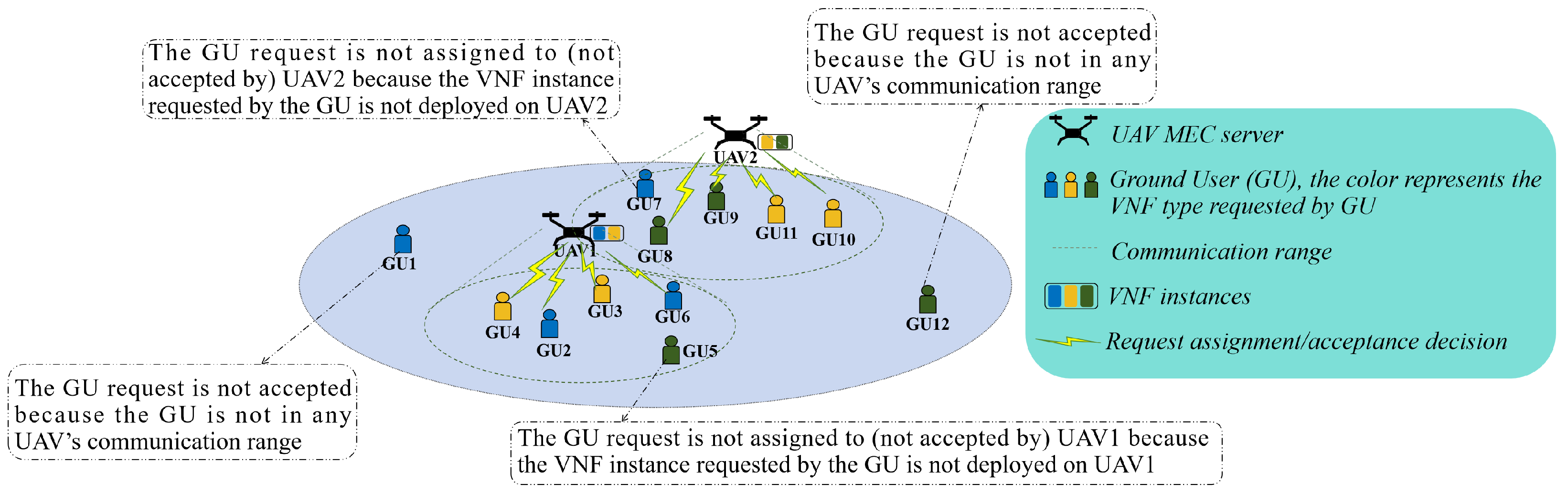
3.1. Network Architecture Model

We consider a multi-UAV mobile-edge network in which M UAVs, denoted by the set $\mathcal{M}$ = {1, 2, …, M}, act as mobile-edge servers to provide VNF services for K GUs, denoted by the set $\mathcal{K}$ = {1, 2, …, K}; F VNFs denoted by $\mathcal{F}$ = {$f^1$, $f^2$, …, $f^F$} are provided. Each GU has real-time and changing VNF requests during period T. Specifically, and for simplicity, T is equally divided into T time frames, and the length $\tau$ = T / T of each time frame t∈$\mathcal{T}$ = {1, 2, …, T} is short enough that decisions made in one time frame can be considered real time. We assume that each GU generates a VNF request at the beginning of each time frame. $r_k^t$ = ($f_k^{i,t}$, $B_k^t$) is used to represent the GU k’s (k∈$\mathcal{K}$) request in the tth time frame, where $f_k^{i,t}$ denotes that VNF $f^i$∈$\mathcal{F}$ is requested by GU k in the tth time frame (t∈$\mathcal{T}$); $B_k^t$ denotes the data size needed to be processed in the tth time frame. Because the requests are generated in real time, in the tth time frame, the requests after the tth time frame are not known.

UAV m ∈$\mathcal{M}$ has $C_m$ computing resources to deploy shared VNFs. A binary decision variable $d_{m,vnf}^{i,t}$ is used to indicate whether VNF $f^i$ is deployed on UAV m in the tth time frame. If VNF $f^i$ is deployed on UAV m in the tth time frame, $d_{m,vnf}^{i,t}$ = 1. Otherwise, $d_{m,vnf}^{i,t}$ = 0. $C_{ins}^i$ denotes the computing resources required for VNF $f^i$ instantiation. Because of the computing resources constraint, in each time frame, the resources that are needed by VNF instances deployed on UAV m should not be more than those possessed by UAV m, so

$$C1:\sum _{i=1}^F{C}_{ins}^i·d_{m,vnf}^{i,t}\le C_m.$$

(1)

An illustrative example of a multi-UAVs mobile-edge network is shown in Figure 1.

3.2. GU and UAV Mobility Model

GUs and UAVs are continuously mobile, but for simplicity, we assume that their locations are fixed in a time frame because the duration of a time frame is short enough. As such, the three-dimensional (3D) Cartesian coordinate system is used to represent GU and UAV locations.

3.2.1. GU Mobility Model

The location of GU k in the tth time frame is represented by $q_{k,user}^t$ = ($x_{k,user}^t$, $y_{k,user}^t$, 0), and we assume that GUs are mobile within a square area with a side length of $l_{max}$, so that the following is satisfied:

$$C2:0\le x_{k,user}^t\le l_{max},0\le y_{k,user}^t\le l_{max}.$$

(2)

In addition, the mobile velocity $v_{k,user}^t$ of GU k in the tth time frame can be expressed as

$$v_{k,user}^t=\left\{\begin{array}{c}0,t=1\hfill \\ \frac{\parallel q_{k,user}^t-q_{k,user}^{t-1}\parallel }{\tau },t\in \{2,3,\dots ,T\}\hfill \end{array}\right..$$

(3)

Each GU’s mobile velocity cannot exceed the GU’s mobile maximum velocity $v_{user}^{max}$, i.e.,

$$C3:v_{k,user}^t\le v_{user}^{max}.$$

(4)

The GUs’ mobile is random; in the tth time frame, the GUs’ locations after the tth time frame are not known.

3.2.2. UAV Mobility Model

The location of UAV m in the tth time frame is represented by $q_{m,uav}^t$ = ($x_{m,uav}^t$, $y_{m,uav}^t$, H), where H is the UAV’s flight altitude and is assumed to be identical and fixed for all UAVs. We assume that UAV m takes off from a predetermined initial location $q_{m,uav}^s$ = ($x_{m,uav}^s$, $y_{m,uav}^s$, H). A virtual time frame 0 is introduced, and UAV m’s initial location is location $q_{m,uav}^0$ of UAV m in time frame 0, i.e.,

$$C4:q_{m,uav}^0=q_{m,uav}^s.$$

(5)

This assumption more clearly expresses the continuity of a UAV’s trajectory in time, which is convenient for later calculation and problem formulation. The velocity $v_{m,uav}^t$ of UAV m in the tth time frame cannot exceed the UAV’s maximum velocity $v_{uav}^{max}$, i.e.,

$$C5:v_{m,uav}^t=\frac{\parallel q_{m,uav}^t-q_{m,uav}^{t-1}\parallel }{\tau }\le v_{uav}^{max},t\in \mathcal{T}.$$

(6)

Additionally, the distance $d_{m1,m2}^{t,uav}$ = $\parallel q_{m1,uav}^t-q_{m2,uav}^t\parallel$ (m1≠m2, t∈$\mathcal{T}$) between UAV m1 and UAV m2 in the tth time frame should be no less than the UAVs’ minimum safe distance $d_{uav}^{min}$ to prevent collision, which means

$$C6:d_{m1,m2}^{t,uav}\le d_{uav}^{min},m1\ne m2.$$

(7)

3.3. Request Admission Model

Assuming that each request’s real-time delay requirement is no more than a time frame’s duration $\tau$, the admission decision (accepted or rejected by a UAV) of request $r_k^t$ which is generated by GU k at the beginning of the tth time frame should be made in the tth time frame. Then, a binary decision variable $A{c}_{k,m}^t$ is introduced to indicate whether request $r_k^t$ is accepted by UAV m in the tth time frame. If request $r_k^t$ is accepted by UAV m in the tth time frame, $A{c}_{k,m}^t$ = 1. Otherwise, $A{c}_{k,m}^t$ = 0. A request can be accepted by no more than one UAV, so

$$C7:\sum _{m=1}^{M}A{c}_{k,m}^t\le 1.$$

(8)

When ${\sum }_{m=1}^{M}A{c}_{k,m}^t=0$, it means $r_k^t$ is not accepted by any UAV, i.e., request $r_k^t$ is rejected.

To complete the acceptance of requests generated at the tth time frame, during the tth time frame, GUs should offload request data to UAVs, UAVs use VNF instances to process request data, and UAVs send back the result to the GUs. For this process, we assume that (1) the resulting data size of a request is much smaller than that of the data that need to be processed, so the time needed for UAVs sending data back to GUs can be ignored, and (2) each UAV evenly divides time frame t into two time slots and the length of each time slot is $\frac{\tau }{2}$. The former time slot is used for GUs’ offloading requests, and the latter time slot is used for the UAV processing requests. The time division of a UAV is shown in Figure 2. We next explain request offloading and processing.

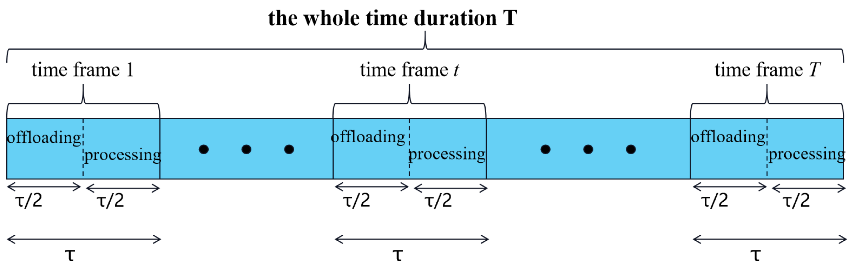
3.3.1. Request Offloading

In the tth time frame, if UAV m accepts GU k’s request, GU k must offload the request to UAV m, and GU k needs to be within communication range of UAV m, i.e.,  

$$C8:A{c}_{k,m}^t·d_{k,m}^{t,user}\le d_{comm}^{max},$$

(9)

where $d_{k,m}^{t,user}$ = $\parallel q_{k,user}^t-q_{m,uav}^t\parallel$ is the distance between GU k and UAV m in the tth time frame, and $d_{comm}^{max}$ is the maximum UAV communication distance.

Regarding the communication channel for offloading, because we assume that line-of-sight (LoS) links dominate the wireless channel between GUs and UAVs, the free-space path-loss model is used to model the channel. The channel power gain $h_{k,m}^t$ between GU k and UAV m in the tth time slot can be calculated as $g_0{\left(d_{k,m}^{t,user}\right)}^{-2}$, where $g_0$ is the path loss at a reference distance of 1 m. Each UAV has a W MHz bandwidth for GUs offloading data to it, and the UAV adopts frequency division multiplexing to receive multiple GUs’ offloading in the same time frame’s offloading time slot. Then, introducing a decision variable ${\alpha w}_{k,m}^t$ indicates the bandwidth proportion that UAV m allocates to GU k for offloading in the tth time frame. In the tth time frame, only when GU k needs offload to UAV m is it necessary for UAV m to allocate bandwidth to GU k, so that

$$C9:{\alpha w}_{k,m}^t\le A{c}_{k,m}^t.$$

(10)

Thus, the offloading rate $R{O}_{k,m}^t$, and offloading data size $B{O}_{k,m}^t$ that GU k offloads to UAV m in the tth time frame are, respectively, expressed as

$$R{O}_{k,m}^t={\alpha w}_{k,m}^{t}Wlo{g}_2(1+\frac{P_{k,m}{h}_{k,m}^t}{{\alpha w}_{k,m}^{t}W{N}_0}),B{O}_{k,m}^t=R{O}_{k,m}^t·\frac{\tau }{2},$$

(11)

where $P_{k,m}$ is the transmission power from GU k offloading to UAV m, and $N_0$ is the noise power spectral density. The offloading data size $B{O}_{k,m}^t$ should be no less than $B_k^t$ to ensure all data are offloaded if UAV m accepts GU k’s requests in the tth time frame, so

$$C10:B{O}_{k,m}^t\ge A{c}_{k,m}^t·B_k^t.$$

(12)

In the tth time frame, the bandwidth that UAV m allocates to GUs is no more than the bandwidth of UAV m, i.e.,

$$C11:\sum _{k=1}^K{\alpha w}_{k,m}^t\le 1.$$

(13)

3.3.2. Request Processing

To facilitate subsequent problem formulation, a binary auxiliary variable $a_k^{i,t}$ is used to indicate whether $r_k^t$ = ($f_k^{i,t}$, $B_k^t$) generated by GU k requests VNF $f^i$ in the tth time frame. If $r_k^t$ requests VNF $f^i$ in the tth time frame, $a_k^{i,t}$ = 1. Otherwise, $a_k^{i,t}$ = 0. Because requests can only be processed by the VNF instances on UAVs, if UAV m accepts $r_k^t$ = ($f_k^{i,t}$, $B_k^t$) in the tth time frame, VNF instance $f^i$ must be deployed on UAV m in the tth time frame, so

$$C12:A{c}_{k,m}^t·a_k^{i,t}·d_{m,vnf}^{i,t}=A{c}_{k,m}^t·a_k^{i,t}.$$

(14)

From the above, we know that the length of the processing time slot in each time frame is $\frac{\tau }{2}$, and the VNF $f^i$ instance has $C_{ins}^i$ instantiation computing resources, which can be used to process data. Thus, if UAV m deploys VNF instance $f^i$ in a time frame, it has $C_{ins}^i·\frac{\tau }{2}$ available computing resources in the time frame to process requests requiring $f^i$. Additionally, if UAV m does not deploy VNF instance $f^i$ in a time frame, it has no available computing resources in the time frame to process requests requiring $f^i$. Then, a decision variable ${\alpha c}_{k,m}^{i,t}$ is introduced to indicate the proportion of VNF $f^i$ instance’s available computing resources that UAV m allocates to request $r_k^t$. Only when UAV m accepts $r_k^t$ and $r_k^t$ requests $f^i$ is it necessary for UAV m to allocate VNF $f^i$ instance’s computing resources to GU k in the tth time frame, i.e.,  

$$C13:{\alpha c}_{k,m}^{i,t}\le A{c}_{k,m}^t·a_k^{i,t}.$$

(15)

We use $C_U$ to represent the number of CPU cycles required for processing a data bit. The data bits $B{P}_{k,m}^{i,t}$ used by UAV m’s VNF $f^i$ instance’s computing resources to process request $r_k^t$ can be calculated as

$$B{P}_{k,m}^{i,t}=\frac{{\alpha c}_{k,m}^{i,t}{d}_{m,vnf}^{i,t}\frac{\tau }{2}{C}_{ins}^i}{C_U}.$$

(16)

The data bits $B{P}_{k,m}^{i,t}$ should be no less than $B_k^t$ to ensure all data are processed if UAV m accepts request $r_k^t$ and the $r_k^t$ requests VNF $f^i$ in the tth time frame, i.e.,

$$C14:B{P}_{k,m}^{i,t}\ge A{c}_{k,m}^t·a_k^{i,t}·B_k^t.$$

(17)

To ensure the constraint of computing resources is met, for UAV m, its VNF $f^i$ instance’s computing resources allocated to GUs should not be more than it has in the tth time frame, so that

$$C15:\sum _{k=1}^K{\alpha c}_{k,m}^{i,t}\le d_{m,vnf}^{i,t}.$$

(18)

3.4. UAV Energy Consumption Model

UAVs consume energy for computing and flight propulsion.

3.4.1. Computing Energy Consumption

$P_U$ is introduced to represent the energy consumption for each CPU cycle. In the tth time frame, the computed bits $B_{m,com}^t$ and computing energy consumption $E_{m,com}^t$ of UAV m can be calculated as

$$B_{m,com}^t=\sum _{k=1}^{K}A{c}_{k,m}^t·B_k^t,E_{m,com}^t=B_{m,com}^t·C_U·P_U$$

(19)

Thus, the computing energy consumption $E_{com}^t$ of all UAVs in the tth time frame and the total computing energy consumption $E_{com}^{total}$ during the whole time duration T are

$$E_{com}^t=\sum _{m=1}^M{E}_{m,com}^t,E_{com}^{total}=\sum _{t=1}^T{E}_{com}^t.$$

(20)

3.4.2. Flight Propulsion Energy Consumption

According to [46], the flight propulsion power $P_m^t$ of UAV m in the tth time frame is related to the velocity $v_{m,uav}^t$, which can be expressed as

$$\begin{array}{cc}\hfill P_m^t=& P_0(1+\frac{3\parallel v_{m,uav}^t{\parallel }^2}{U_{tip}^2})+P_i{(\sqrt{1+\frac{{\parallel v_{m,uav}^t\parallel }^4}{4{v_0}^4}}-\frac{{\parallel v_{m,uav}^t\parallel }^2}{2{v_0}^2})}^{\frac{1}{2}}\hfill \\ & +\frac{1}{2}{d}_0\epsilon s{M}_{rotor}{\parallel v_{m,uav}^t\parallel }^3,\hfill \end{array}$$

(21)

where $P_0$, $P_i$, $U_{tip}$, $v_0$, $d_0$, s, $\epsilon$, and $M_{rotor}$ represent the blade profile power, induced power of UAV in hovering status, the rotor blade tip speed, the mean-rotor-induced velocity in forward flight, the fuselage drag ratio, rotor solidity, the air density, and rotor disc area, respectively. The flight propulsion energy consumption $E_{m,fly}^t$ of UAV m in the tth time frame can be calculated as

$$E_{m,fly}^t=P_m^t·\tau .$$

(22)

Thus, the flight propulsion energy consumption $E_{fly}^t$ of all UAVs in the tth time frame and the total flight propulsion energy consumption $E_{fly}^{total}$ during the whole time duration T which cosisting of T time frames are

$$E_{fly}^t=\sum _{m=1}^M{E}_{m,fly}^t,E_{fly}^{total}=\sum _{t=1}^T{E}_{fly}^t.$$

(23)

From the above, we know that during the whole time duration T which cosisting of T time frames, the total energy consumption $E^{total}$ of all UAVs is expressed as

$$E^{total}=E_{com}^{total}+E_{fly}^{total}.$$

(24)

3.5. Cost of UAVs’ Model for Accepting Requests

The cost includes two parts, namely, the instantiation cost produced when UAVs deploy VNF instances and the computing cost produced when UAVs use VNF instances to process GU requests.

3.5.1. Instantiation Cost

We assume that (1) no VNF instance is deployed on any UAV at the beginning of the time duration T which cosisting of T time frames, which is called initial VNF deployment; (2) the initial VNF deployment is the VNF deployment {$d_{m,vnf}^{i,0}$|m∈$\mathcal{M}$, $f^i$∈$\mathcal{F}$} in the introduced virtual time frame 0, so that

$$C16:d_{m,vnf}^{i,0}=0,m\in \mathcal{M},f^i\in \mathcal{F}.$$

(25)

A constant $C_{ins}^i$ is used to represent the instantiation cost of deploying VNF $f^i$. In the tth time frame ($t\in \mathcal{T}$), if UAV m does not deploy the VNF $f^i$ instance, a UAV m deploying VNF $f^i$ incurs no instantiation cost. If UAV m deploys a VNF $f^i$ instance in the tth time frame ($t\in \mathcal{T}$), the instantiation cost of UAV m deploying VNF $f^i$ depends on whether VNF $f^i$ instance is deployed on UAV m in the (t − 1)th time frame: (a) if VNF $f^i$ instance is deployed on UAV m in the (t − 1)th time frame, the instantiation cost of UAV m deploying VNF $f^i$ is 0; (b) if the VNF $f^i$ instance is not deployed on UAV m in the (t − 1)th time frame, the instantiation cost of UAV m deploying VNF $f^i$ is $C_{ins}^i$. Thus, the instantiation cost $c_{m,ins}^t$ of UAV m deploying VNF instances in the tth time frame can be expressed as

$$c_{m,ins}^t=\sum _{i=1}^F{d}_{m,vnf}^{i,t}·(d_{m,vnf}^{i,t}-d_{m,vnf}^{i,t-1})·C_{ins}^i,t\in \mathcal{T}.$$

(26)

Thus, the instantiation cost $c_{ins}^t$ of all UAVs deploying VNF instances in the tth time frame and the total instantiation cost $c_{ins}^{total}$ during the whole time duration T which cosisting of T time frames are

$$c_{ins}^t=\sum _{m=1}^M{c}_{m,ins}^t,c_{ins}^{total}=\sum _{t=1}^T{c}_{ins}^t.$$

(27)

3.5.2. Computing Cost

A constant $C_{com}^i$ is used to represent the computing cost of the VNF $f^i$ instances per CPU cycle to process data. In the tth time frame, the computing cost $c_{m,com}^t$ of UAV m processing requests is

$$c_{m,com}^t=\sum _{k=1}^K\sum _{i=1}^{F}A{c}_{k,m}^t·a_k^{i,t}·B_k^t·C_U·C_{com}^i.$$

(28)

Thus, the computing cost $c_{com}^t$ of all UAVs’ processing requests in the tth time frame and the total processing cost $c_{com}^{total}$ during the whole time duration T which cosisting of T time frames is

$$c_{com}^t=\sum _{m=1}^M{c}_{m,com}^t,c_{com}^{total}=\sum _{t=1}^T{c}_{com}^t.$$

(29)

Based on the above, during the whole time duration T which cosisting of T time frames, the total cost $c^{total}$ of all UAVs accepting requests is expressed as

$$c^{total}=c_{ins}^{total}+c_{com}^{total}.$$

(30)

3.6. Problem Formulation

The aim of the problem is to maximize the number of accepted requests while minimizing both the energy consumption and the cost of accepting requests within the constraints of UAV resources and real-time request latency. To achieve this, the optimization of joint VNF deployment ${\mathcal{D}}_{\mathcal{V}\mathcal{N}\mathcal{F}}$ = {$d_{m,vnf}^{i,t}$|m∈$\mathcal{M}$, $f^i$∈$\mathcal{F}$, t∈$\mathcal{T}$} and multiple UAV trajectory planning $\mathcal{Q}$ = {$q_{m,uav}^t$|m∈$\mathcal{M}$, t∈$\mathcal{T}$} is important. Additionally, during the whole time duration T, request admission decision $\mathcal{AC}$ = {$A{c}_{k,m}^t$|k∈$\mathcal{K}$, m∈$\mathcal{M}$, t∈$\mathcal{T}$}, resource allocation decision ${\mathcal{AR}}_{\mathcal{W}}$ = {${\alpha w}_{k,m}^t$|k∈$\mathcal{K}$, m∈$\mathcal{M}$, t∈$\mathcal{T}$}, and ${\mathcal{AR}}_{\mathcal{C}}$ = {${\alpha c}_{k,m}^{i,t}$|k∈$\mathcal{K}$, m∈$\mathcal{M}$, $f^i$∈$\mathcal{F}$, t∈$\mathcal{T}$} should be optimized. Then, the proposed problem can be formulated as a nonconvex mixed integer nonlinear programming problem as follows:

$$\begin{array}{c}\hfill \underset{\genfrac{}{}{0pt}{}{\mathcal{Q},{\mathcal{D}}_{\mathcal{V}\mathcal{N}\mathcal{F}},}{\mathcal{AC},{\mathcal{AR}}_{\mathcal{W}},{\mathcal{AR}}_{\mathcal{C}}}}{\max }Coe{f}_1^P·\sum _{t=1}^T\sum _{m=1}^M\sum _{k=1}^{K}A{c}_{k,m}^t-Coe{f}_2^P·({\omega }_c·c^{total}+{\omega }_e·E^{total}),\end{array}$$

(31)

subject to

C1-C16,

$$d_{m,vnf}^{i,t},A{c}_{k,m}^t\in \{0,1\},k\in \mathcal{K},m\in \mathcal{M},f^i\in \mathcal{F},t\in \mathcal{T},$$

(32)

$${\alpha w}_{k,m}^t,{\alpha c}_{k,m}^{i,t}\in [0,1],k\in \mathcal{K},m\in \mathcal{M},f^i\in \mathcal{F},t\in \mathcal{T},$$

(33)

where $Coe{f}_1^P$ represents the priority coefficient of the number of accepted requests, and $Coe{f}_2^P$ represents the priority coefficient of the weighted sum of the energy consumption and cost. The two priority coefficients are used to ensure that maximizing the number of accepted requests is the first priority. Additionally, ${\omega }_e$ and ${\omega }_c$, respectively, represent the weights of energy consumption and the cost, and ${\omega }_e$ + ${\omega }_c$ = 1. Problem formulation (1) has both discrete and continuous variables; problem formulation (2) has nonconvex formulas. Thus, solving the problem is difficult.

4. Problem Solution

From the above, the proposed problem is hard to solve because it includes both discrete and continuous variables and because of its nonconvexity. We can further formulate it as a Markov decision process by analyzing the problem’s characteristics. We thus developed an improved DRL algorithm, which is called an online DRL algorithm, based on jointly optimizing discrete and continuous actions, as the solution to handle the problem. The proposed algorithm was designed for centralized (single-agent) and decentralized (multi-agent) scenarios. In the single-agent case, the agent can be a terrestrial base station or an additional introduced UAV that controls the UAVs acting as servers; for the multi-agent case, each UAV that acts as the server is an agent. In both the single- and multi-agent cases, each agent can obtain all information in the environment. The difference between the cases is that in the case of a single agent, the agent generates the VNF deployments and trajectory planning of all UAVs. In the multi-agent case, one agent controls one UAV; that is, an agent generates its corresponding UAVs’ VNF deployments and trajectory planning. We will study the case where an agent in the multi-agent case can only obtain partial information in future work.

4.1. The Key Idea of the Proposed Algorithm

The key idea of the proposed algorithm is establishing the coupled influence between VNF deployment (discrete action) and UAV trajectories’ planning (continuous action). Specifically, when making the VNF deployment (discrete action) decision, UAV trajectory planning (continuous action) is considered, and vice versa. In our algorithm, the two keys are reflected in the design of the neural networks and the training process to achieve the key aims. Figure 3 shows the structure of the proposed algorithm in the centralized scenario (the single-agent case), in which the Online-VNF-Qnetwork is used to generate all UAVs’ discrete actions (VNF deployment), the UAVs-Trajectories Actor Network is used to generate all UAVs’ continuous actions (trajectories), and the Critic Network is used to criticize all actions generated by the agent. The structure for one agent of the proposed algorithm in the decentralized scenario (the multi-agent case) is similar to that in Figure 3. The difference is that each agent in the multi-agent scenario can only generate discrete actions (VNF deployments) of its corresponding UAV using Online-VNF-Qnetwork in its structure and generate the continuous actions (trajectories) of its corresponding UAV using the UAVs-Trajectories Actor Network. The Critic Network can only be used to criticize the actions it generates.

Because the inputs of a neural network affect its outputs, neural network design is key to reflecting and establishing the effect of the coupling of discrete and continuous actions. Specifically, continuous action is taken as one part of the input to the Online-VNF-Qnetwork; similarly, discrete action is taken as one part of the input of the UAVs-Trajectories Actor Network, where the Online-VNF-Qnetwork and UAVs-Trajectories Actor Network are used to obtain discrete and continuous actions, respectively.

The role of the training process is the joint optimization of VNF deployment and UAV trajectory planning by learning the coupling relationship between the two processes to determine the optimal target. The general training idea is as follows. In our setting, a complete action includes a discrete action (VNFs deployment) and a continuous action (UAVs’ trajectories planning). When training the Online-VNF-Qnetwork, the reward decided by a complete action rather than the reward decided by only the discrete action is used to fine-tune discrete action. Thus, after training, the choice of a discrete action considers the discrete action and its corresponding continuous action. As the method for calculating the reward used to train the UAVs-Trajectories Actor Network is complicated, we describe it later. What we emphasize here is that the reward is also decided by the complete action rather than only by the continuous action. Thus, when learning to adjust the choice of the continuous action, the adjustment is influenced by both discrete and continuous actions. After training, the choice of a continuous action considers both continuous and discrete actions.

Additionally, although a complete action includes a discrete action and a continuous action, whose selection is based on their coupled effect, we assume that the execution and selection of discrete and continuous actions are sequential. In a complete action, the discrete action is selected/executed before a continuous action. On this basis, we created a design to narrow the UAV flying option range, which reflects the influence of discrete action on continuous action. A detailed description of this design is provided next.

4.2. Environment State

We describe the information contained in the state using the notations in Section 3:

➀ The current time frame t, where t ∈$\mathcal{T}$.

➁ The VNF deployment. For the state in the tth time frame, its VNF deployment is {$d_{m,vnf}^{i,t-1}$|m∈$\mathcal{M}$, $f^i$∈$\mathcal{F}$}. In the first state, the UAV locations are the locations in time frame 0, so none of the UAVs deploy any VNF instance, which meets constraint C16.

➂ The UAV locations. For the state in the tth time frame, the UAV locations are {$q_{m,uav}^{t-1}$|m∈$\mathcal{M}$}. (1) In the first state, the UAV locations are the locations in time frame 0, which are also their initial locations. Thus, constraint C4 is met. (2) We assume that the UAV initial location setting satisfies the minimum safe distance constraint C6.

➃ The GU locations. For the state in the tth time frame, the GU locations are {$q_{k,user}^t$|k∈$\mathcal{K}$}. The GU locations are randomly generated with constraints C2 and C3.

➄ The GUs’ VNF requests. For the state in the tth time frame, the GUs’ VNF requests are {$r_k^t$|k∈$\mathcal{K}$}.

➅ GU sorting: GUs are sorted according to their distance from the coordinate origin from near to far in the first time frame, setting the lower left corner as the coordinate origin.

4.3. Reward

Before describing the reward calculation method, we should note that the state/info/ reward feedback from the environment received by the agent is the same regardless of whether the agent is in the single-agent case or in the multi-agent case, that is, the state/info/reward generated after all UAVs execute their corresponding actions. This is because, in the multi-agent case, the actions generated between agents should be cooperatively executed. Thus, an agent should receive not only the executing feedback of actions only generated by itself but also the executing feedback of actions generated by all agents. Therefore, the reward described in this subsection is applicable to both single- and multi-agent situations.

Based on the problem target and the goal of DRL, in the tth state, the reward $Rewar{d}_t$ obtained after executing the complete action is defined as

$$Rewar{d}_t=Coe{f}_1^P·(N_{acc}^t-N_{una}^t)-Coe{f}_2^P·({\omega }_e·(E_{com}^t+E_{fly}^t)+{\omega }_c·(c_{ins}^t+c_{com}^t)),$$

(34)

where $N_{acc}^t$/$N_{una}^t$ is the number of accepted/unaccepted GU requests in the tth state achieved by executing the complete action. $N_{acc}^t$ is counted using ${\sum }_{m=1}^M{\sum }_{k=1}^{K}A{c}_{k,m}^t$, and $N_{una}^t$ as computed by K - $N_{acc}^t$. $Coe{f}_1^P·(N_{acc}^t-N_{una}^t)$ means providing a positive reward for accepting a request and a negative reward for rejecting a request. This setting further encourages the acceptance of requests.

From the above, we assume that a discrete action is selected before that of a continuous action, but the reward of a discrete action is not decided by itself but by the reward of the complete action. In other words, $Rewar{d}_t$, which is computed in consideration of both discrete and continuous actions, is used as the reward for discrete action. Thus, when training the Online-VNF-Qnetwork to choose a discrete action, it considers the continuous action influenced by the discrete action.

After deciding upon a discrete action, the discrete action and current UAV locations are together used to narrow the UAV flying option range. When narrowing the flying option range, an integer $N_{comb}^t$ is generated, whose generation method is described in the Action Selection and Execution Process section. The reward Reward_CA = $Coe{f}_1^P·(N_{acc}^t-N_{comb}^t)-Coe{f}_2^P·({\omega }_e·(E_{com}^t+E_{fly}^t)+{\omega }_c·(c_{ins}^t+c_{com}^t))$ is used to as the reward for continuous action. First, we use $N_{acc}^t-N_{comb}^t$ rather than $N_{acc}^t-N_{una}^t$ because $N_{acc}^t$ is a basic accepted number reference found when narrowing the flying option range, $N_{acc}^t$ is the near-optimal or optimal accepted number of requests under the corresponding discrete action. A reference computing reward can be used to more accurately evaluate the request acceptance situation. Second, the cost and energy consumption are decided by both discrete and continuous actions. So, when training the UAVs-Trajectories Actor Network to choose continuous action, it considers the corresponding discrete action.

4.4. The Single-Agent Case in Centralized Scenario

This subsection introduces the implementation of the single-agent case in the centralized scenario.

4.4.1. Neural Network

Figure 3 shows that our proposed algorithm comprises three kinds of neural networks, Online-VNF-Qnetwork, UAVs-Trajectories Actor Network, and Critic Network, which are introduced in detail next.

• Online-VNF-Qnetwork: This neural network is used to obtain discrete actions (VNF deployment in the current time frame). Its input State_DA and its output DA_ID/DA are as follows: (a) State_DA includes state information ➁–➄, where the information about GUs is sorted by ➅. (b) DA_ID/DA: DA_ID is an integer representing a discrete action (DA, VNF deployment). Note that (1) DA_ID ∈ {0, 1, …, $N_{DA}-$1}, where $N_{DA}$ is the number of all VNF deployments (DA) on all UAVs that satisfy computing resource constraint C1; (2) all VNF deployments (DA) in all UAVs that satisfy computing resource constraint C1 and $N_{DA}$ are obtained via preprocessing.
• UAVs-Trajectories Actor Network: This neural network is used to obtain continuous actions (CAs, the UAV flying action). Its input State_CA and its output CA are as follows: (a) State_CA includes the new VNF deployment obtained by using DA to change ➁, state information ➂–➄, where the information about GUs is sorted using ➅. (b) CA includes 2 · M continuous variables. These continuous variables and the DA together determine the next location of the UAVs, which is described in detail in the Action Selection and Execution Process Section.
• Critic Network: This neural network is used in the training process to evaluate the quality of the continuous action. Its input State_Cri and its output Q_Cri are as follows: (a) State_Cri includes state information ➁–➄, where the information about GUs is sorted by ➅, the DA and the CA. (b) Q_Cri is a a real number used to evaluate the continuous action’s quality.

4.4.2. Action Selection and Execution Process

The action-selection and -execution processes are indicated by the black solid lines in Figure 3, and we explain this process in detail next.

In the action selection process, first, the agent obtains state information from the environment. Second, based on the State_DA obtained from state information, the DA_ID is obtained by the Online-VNF-Qnetwork, which knows the DA. Next, State_CA is computed using state information and the DA, and the UAVs-Trajectories Actor Network is used to obtain the CA based on State_CA. Finally, the agent combines the DA and CA into a complete action and returns the complete action to the environment.

The action execution process is as follows. When the environment in the tth state receives the complete action from the agent, the DA and CA are extracted from the complete action. Then, ➁ changes based on the DA, and, simultaneously, reward $R_{cost}^{ins,t}$ = −$Coe{f}_2^P·{\omega }_c·c_{ins}^t$ for the instantiation cost is computed. Next, the new UAV locations are computed, and the computing steps are as follows: (1) For UAV m∈$\mathcal{M}$, the area to which it can fly (a circle with its current location as the center and the maximum moving distance $v_{uav}^{max}·\tau$ as the radius) is divided into multiple subgrids with side length $l_{grid}$. Assume that there are $N_{node}$ grid nodes in the circle area and the circle center is one of the grid nodes. The locations of $N_{node}$ grid nodes for UAV m are called UAV m’s flying optional locations. Then, $N_{node}^M$ combinations exist for all mobile UAVs. (2) The optimal combination is found by examining all combinations. The target value computed using Equation (31) of the optimal combination is the maximum among all possible combinations. Then, we can know that the number of GU requests the optimal combination is accepting is $N_{comb}^t$. (3) The UAVs’ temporary next locations are found. For each UAV, its narrowed moving/flying option range is a circle, the center of which is obtained from the optimal combination, which has a radius that is the smaller of $l_{grid}$ and $Co{n}_{dis}$. $Co{n}_{dis}$ is the maximum flying distance $v_{uav}^{max}·\tau$ in a time frame minus the distance from the UAV’s current location to its moving option range center, which is used to avoid violating velocity constraint C5. (4) The new UAV locations are determined. If no collision occurs based on the UAVs’ temporary next locations, the UAVs’ temporary next locations are the UAVs’ new locations. Otherwise, all new UAV locations are their current location. Thus, the UAVs move only when the minimum safe distance constraint is guaranteed; otherwise, they stay in their current locations. Additionally, their initial locations meet the minimum safe distance constraint C6. Therefore, the minimum safe distance constraint C6 is always met. Next, the new UAV locations are used to update ➂, and the reward $R_{nrj}^{fly,t}$ = −$Coe{f}_2^P·{\omega }_e·E_{fly}^t$ regarding flight-propulsion energy consumption is computed. Then, on the basis of ➃, ➄, and updated ➁ and ➂, it is determined whether each GU request is accepted; if so, it is determined which UAV accepts the request. The method for deciding to accept a GU request is as follows. First, all requests that have not been accepted are marked. No communication or computing resources (computing resources are allocated based on the VNF instances) are allocated to any GU for each UAV, which guarantees constraints C9 and C13 are met. The distances between each UAV and each GU are calculated, and the distances from near to far are sorted. Second, the UAV–GU pair is removed according to the sorted distances, and the following operations are performed. If the distance between the UAV and GU is greater than the communication distance, the GU request acceptance decision is to stop, which guarantees constraint C8 is met. Otherwise, it is determined whether the GU’s request of the UAV–GU pair is marked as accepted; if so, no more operations are performed, and the next UAV–GU pair is removed, which guarantees constraint C7 is satisfied. Otherwise, we determine whether the instance of the VNF requested by the GU is deployed on the UAV in the UAV–GU pair. If not, no more operations are performed, and the next UAV–GU pair is removed, which can guarantee constraint C12 is satisfied. Otherwise, based on the GU data size that needs to be processed, the minimum communication resources required to offload all the data to the UAV are calculated, as are the minimum computing resources that are required to process all the data using the VNF instance requested by GU, which guarantees constraints C10 and C14 are satisfied. Then, we check whether the remaining communication resources of the UAV are no less than the minimum communication resources required by the GU and whether the remaining computing resources of the instance of the VNF requested by the GU deployed on the UAV instance are no less than the minimum computing resources required by the GU. If either of the remaining resources is insufficient, no more operations are performed, and the next UAV–GU pair is removed, which guarantees constraints C11 and C15 are satisfied. Otherwise, the GU’s request is accepted by the UAV. Thus, the GU’s request is marked as accepted; the rewards $R_{nrj}^{com,t}$ = −$Coe{f}_2^P·{\omega }_e·E_{com}^t$ and $R_{cost}^{com,t}$ = −$Coe{f}_2^P·{\omega }_c·c_{com}^t$ for computing energy and computing cost for processing the request should be computed, respectively. When deciding whether each request is accepted, the total number of accepted requests $N_{acc}^t$ in this state is counted. After the GU request acceptance decision, the total number of unaccepted requests $N_{una}^t$ in this state can be computed. Then, based on $N_{acc}^t$ and $N_{una}^t$, the reward for request acceptance is computed as $Coe{f}_1^P$· ($N_{acc}^t$−$N_{una}^t$). At this point, the complete action in this state is executed, so the reward of this completed action is computed by adding the rewards mentioned above. Then, all rewards, $N_{comb}^t$ and $N_{acc}^t$, are returned to the agent. If t≤ T, ➃ is updated with GU mobility constraints, and ➄ is randomly generated, which means the next state/time frame is entered. Otherwise, the termination state is reached. In the action-execution process, some fixed methods are used to avoid the violation of constraints.

4.4.3. Training Process

The training process for the single-agent case is shown in all lines in Figure 3, and its pseudo-code is shown in Algorithm 1.

Algorithm 1 The algorithm for the training of the single-agent case.

1: Initialize Online-VNF-Qnetwork $Q^d(·)$, UAVs-Trajectories Actor Network $\pi (·)$, and Critic Network $Q^c(·)$ with parameters ${\theta }_Q$, ${\theta }_{Act}$, ${\theta }_{Cri}$; Initialize Target Online-VNF-Qnetwork ${\widehat{Q}}^d(·)$, Target UAVs-Trajectories Actor Network $\widehat{\pi }(·)$, and Target Critic Network ${\widehat{Q}}^c(·)$ with parameters ${\widehat{\theta }}_Q$ = ${\theta }_Q$, ${\widehat{\theta }}_{Act}$ = ${\theta }_{Act}$ and ${\widehat{\theta }}_{Cri}$ = ${\theta }_{Cri}$; Initialize replay memory buffer $\mathcal{D}$. 2: for episode = 1,…,$Episod{e}_{max}$ do 3:     Initialize the state generating $stat{e}_1$; initialize a random process $\mathcal{N}$ for continuous action exploration. 4:     for t = 1,…,T do 5:        With probability $\epsilon$ select a random discrete action $a_{dis}^t$; 6:        Otherwise, obtain $State\_D{A}_t$ based on $stat{e}_t$ and then select $a_{dis}^t$ = $argma{x}_{a_{dis}}{Q}^d(State\_D{A}_t,a_{dis}|{\theta }_Q)$. 7:        Obtain $State\_C{A}_t$ based on $State\_D{A}_t$ and $a_{dis}^t$; 8:        Then select continuous action $a_{con}^t$ = $\pi (State\_C{A}_t|{\theta }_{Act})$ + ${\mathcal{N}}_t$ according to the current policy and exploration noise. 9:        Combine discrete action $a_{dis}^t$ and continuous action $a_{con}^t$ into a complete action $a^t$. 10:       Execute action $a^t$, and obtain $Rewar{d}_t$ and $inf{o}_t$ = [$N_{acc}^t$, $N_{una}^t$, $R_{cost}^{ins,t}$, $R_{nrj}^{fly,t}$, $R_{nrj}^{com,t}$, $R_{cost}^{com,t}$]; observe next state $stat{e}_{t+1}$. 11:       Compute $Reward\_C{A}_t$ = $Coe{f}_1^P·(N_{acc}^t-N_{comb}^t)$ + $R_{cost}^{ins,t}$ + $R_{nrj}^{fly,t}$ + $R_{nrj}^{com,t}$ + $R_{cost}^{com,t}$ and obtain $State\_D{A}_{t+1}$ based on $stat{e}_{t+1}$. 12:       Store transition ($State\_D{A}_t$, $a^t$, $Rewar{d}_t$, $Reward\_C{A}_t$, $State\_D{A}_{t+1}$) into $\mathcal{D}$. 13:       Sample random minibatch of B transitions ($State\_D{A}_b$, $a^b$, $Rewar{d}_b$, $Reward\_C{A}_b$, $State\_D{A}_{b+1}$) from $\mathcal{D}$; abstract $a_{dis}^b$ and $a_{con}^b$ from $a^b$. 14:       Select $a_{dis}^{b+1}$ = $argma{x}_{a_{dis}}{\widehat{Q}}^d(State\_D{A}_{b+1},a_{dis}|{\widehat{\theta }}_Q)$; obtain $State\_C{A}_{b+1}$ based on $State\_D{A}_{b+1}$ and $a_{dis}^{b+1}$. 15:       Set $targe{t}_b^{cri}$ = $Reward\_C{A}_b+\gamma {\widehat{Q}}^c(State\_D{A}_{b+1}+a_{dis}^{b+1},\widehat{\pi }(State\_C{A}_{b+1}|{\widehat{\theta }}_{Act})|{\widehat{\theta }}_{Cri})$ 16:       Update parameters ${\theta }_{Cri}$ of the Critic Network $Q^c(·)$ by minimizing its loss function $L\left({\theta }_{Cri}\right)=\frac{1}{B}{\sum }_{b=1}^B{(targe{t}_b^{cri}-Q^c(State\_D{A}_b+a_{dis}^b,a_{con}^b|{\theta }_{Cri}))}^2$ 17:       Obtain $State\_C{A}_b$ based on $State\_D{A}_b$ and $a_{dis}^b$. 18:       Update parameters ${\theta }_{Act}$ of the UAVs-Trajectories Actor Network $\pi (·)$ by using policy gradient approach according to ${\nabla }_{{\theta }_{Act}}J\approx \frac{1}{B}{\sum }_{b=1}^B{\nabla }_{a_{con}}{Q}^c(State\_D{A}_b+a_{dis}^b,a_{con}|{\theta }_{Cri}){|}_{a_{con}=\pi (State\_C{A}_b|{\theta }_{Act})}$; 19:       Set $targe{t}_b^{dis}$ = $Rewar{d}_b+\gamma ma{x}_{a_{dis}}{\widehat{Q}}^d(State\_D{A}_{b+1},a_{dis}|{\widehat{\theta }}_Q)$. 20:       Update parameters ${\theta }_Q$ of the Online-VNF-Qnetwork $Q^d(·)$ by minimizing its loss function according to $L\left({\theta }_Q\right)=\frac{1}{B}{\sum }_{b=1}^B{(targe{t}_b^{dis}-Q^d(State\_D{A}_b,a_{dis}^b|{\theta }_Q))}^2$. 21:       Update three target networks according to ${\widehat{\theta }}_Q={\tau }_{soft}{\theta }_Q+(1-{\tau }_{soft}){\widehat{\theta }}_Q$, ${\widehat{\theta }}_{Cri}={\tau }_{soft}{\theta }_{Cri}+(1-{\tau }_{soft}){\widehat{\theta }}_{Cri}$, ${\widehat{\theta }}_{Act}={\tau }_{soft}{\theta }_{Act}+(1-{\tau }_{soft}){\widehat{\theta }}_{Act}$. 22:     end for 23:   end for note:  In our method, when selecting an action, the focus is on the state information ➁–➅, not the time frame (state information ➀), which can be seen from the three neural networks’ inputting settings. Thus, the time frame used to prompt whether the state is finished is unrelated to the action selection. Then, the action selection of the last time frame can be regarded as the choice of the non-last time frame. So, when setting targets used to update networks, we do not consider the case of the end of the next step.

In the training algorithm, the related neural networks and a replay memory buffer used to store transitions are initialized (Line 1). For each episode, initialize the state generating $stat{e}_1$, and initialize a random process $\mathcal{N}$ to explore continuous actions. Then, for each time frame until the termination state, the first step involves obtaining the transitions (Lines 5–10), which is shown using the solid black and brown lines in Figure 3. In this step, first, select the discrete action $a_{dis}^t$ with the $\epsilon$-greedy strategy. After determining the discrete action, obtain $State\_C{A}_t$ based on $State\_D{A}_t$ and $a_{dis}^t$. Then, select the continuous action $a_{con}^t$ according to the current policy and exploration of noise. Next, the discrete action $a_{dis}^t$ and continuous action $a_{con}^t$ are combined into a complete action $a^t$. Then, $a^t$ is executed, and $Rewar{d}_t$ and $inf{o}_t$ are obtained. Additionally, the next state $stat{e}_{t+1}$ can be observed. The second step involves storing and sampling transitions (Line 11–13), which is shown using a brown dotted line in Figure 3. Before storing a transition, the $Reward\_C{A}_t$ used to train the UAVs-Trajectories Actor Network is computed using $inf{o}_t$, and $State\_D{A}_{t+1}$ is obtained based on $stat{e}_{t+1}$. Then, the transition ($State\_D{A}_t$, $a^t$, $Rewar{d}_t$, $Reward\_C{A}_t$, and $State\_D{A}_{t+1}$) is stored to replay memory buffer $\mathcal{D}$. After sampling the transitions ($State\_D{A}_b$, $a^b$, $Rewar{d}_b$, $Reward\_C{A}_b$, $State\_D{A}_{b+1}$), the discrete actions $a_{dis}^b$ and continuous actions $a_{con}^b$ in $a^b$ are extracted because the discrete and continuous actions need to be separately learned. The last step is the learning process. First, update the parameters of the Critic Network (Lines 14–16), which is shown with a red solid line in Figure 3. Use $State\_D{A}_{b+1}$ and Target Online-VNF-Qnetwork to obtain $a_{dis}^{b+1}$. Then, obtain $State\_C{A}_{b+1}$ based on $State\_D{A}_{b+1}$ and $a_{dis}^{b+1}$. Therefore, the Critic Network is updated by minimizing its loss function

$$\begin{array}{c}\hfill L\left({\theta }_{Cri}\right)=\frac{1}{B}\sum _{b=1}^B{(targe{t}_b^{cri}-Q^c(State\_D{A}_b+a_{dis}^b,a_{con}^b|{\theta }_{Cri}))}^2,\end{array}$$

(35)

where $targe{t}_b^{cri}$ is computed as

$$\begin{array}{c}\hfill targe{t}_b^{cri}=Reward\_C{A}_b+\gamma {\widehat{Q}}^c(State\_D{A}_{b+1}+a_{dis}^{b+1},\widehat{\pi }(State\_C{A}_{b+1}|{\widehat{\theta }}_{Act})|{\widehat{\theta }}_{Cri}).\end{array}$$

(36)

Second, update the parameters of the UAVs-Trajectories Actor Network (Line 17–18), as shown with the red dotted line in Figure 3. $State\_C{A}_b$ should be obtained based on $State\_C{A}_b$, $State\_D{A}_b$, and $a_{dis}^b$. Update the UAVs-Trajectories Actor Network by applying a policy gradient [47], i.e., where $targe{t}_b^{cri}$ is computed as

$$\begin{array}{c}\hfill {\nabla }_{{\theta }_{Act}}J\approx \frac{1}{B}\sum _{b=1}^B{\nabla }_{a_{con}}{Q}^c(State\_D{A}_b+a_{dis}^b,a_{con}|{\theta }_{Cri}){|}_{a_{con}=\pi (State\_C{A}_b|{\theta }_{Act})}.\end{array}$$

(37)

Then, update the parameters of the Online-VNF-Qnetwork (Lines 19–20), which is shown by black dotted lines in Figure 3. The Online-VNF-Qnetwork is updated by minimizing its loss function

$$L\left({\theta }_Q\right)=\frac{1}{B}\sum _{b=1}^B{(targe{t}_b^{dis}-Q^d(State\_D{A}_b,a_{dis}^b|{\theta }_Q))}^2,$$

(38)

where $targe{t}_b^{dis}$ is computed as $targe{t}_b^{dis}=Rewar{d}_b+\gamma ma{x}_{a_{dis}}{\widehat{Q}}^d(State\_D{A}_{b+1},a_{dis}|{\widehat{\theta }}_Q)$. Finally, update the three target networks using ${\widehat{\theta }}_Q={\tau }_{soft}{\theta }_Q+(1-{\tau }_{soft}){\widehat{\theta }}_Q$, ${\widehat{\theta }}_{Cri}={\tau }_{soft}{\theta }_{Cri}+(1-{\tau }_{soft}){\widehat{\theta }}_{Cri}$, ${\widehat{\theta }}_{Act}={\tau }_{soft}{\theta }_{Act}+(1-{\tau }_{soft}){\widehat{\theta }}_{Act}$.

4.4.4. Computational Complexity for Generating Actions/Q-Value

In this subsection, we describe our analysis of the computational complexity of generating the actions/Q-values of the three fully connected neural networks (Online-VNF-Qnetwork, UAVs-Trajectories Actor Network, and Critic Network). The computational complexity of the fully connected neural network is ${\sum }_{ln=1}^{LN-1}n{n}_{ln}·n{n}_{ln+1}$, where LN is the number of the network layers and $n{n}_{ln}$ is the neuron numbers in the lnth layer. $n{n}_{max}={max}_{1\le ln\le LN}n{n}_{ln}$ is the maximum number of neurons among all layers, so $n{n}_{max}^2\ge n{n}_{ln}·n{n}_{ln+1}(n=1,2,\dots ,LN-1)$. Then, $(LN-1)·n{n}_{max}^2\ge {\sum }_{ln=1}^{LN-1}n{n}_{ln}·n{n}_{ln+1}$. Therefore, a fully connected neural network’s computational complexity can be expressed as $\mathcal{O}((LN-1)·n{n}_{max}^2)$. In our setting, our three fully connected neural networks have no more than fiyr hidden layers, which means LN≤ 6. Additionally, their number of hidden layer neurons is a constant between their own input and output numbers, so their $n{n}_{max}$ is the larger of the input and output numbers. For the Online-VNF-Qnetwork, its output number is M·2 + M·F + K·4, and its output number is $N_{DA}^M$. We cannot determine which is bigger iyt of the input and output number, so its computational complexity is $\mathcal{O}\left({(M·F+K+N_{DA}^M)}^2\right)$. As for the UAVs-Trajectories Actor Network, the number of inputs is M·2 + M·F + K·4, and the number of outputs is M·2. Thus, the computational complexity of the UAVs-Trajectories Actor Network is $\mathcal{O}\left({(M·F+K)}^2\right)$. The input and output numbers of the Critic Network are M·5 + M·F + K·4 and 1, respectively. So its computational complexity is $\mathcal{O}\left({(M·F+K)}^2\right)$.

4.5. The Multi-Agent Case in a Decentralized Scenario

This subsection introduces the implementation of the multi-agent case in the decentralized scenario.

4.5.1. Neural Network

In the decentralized scenario, each UAV has an agent for individual UAV action selection. In addition, agent m (m ∈$\mathcal{M}$), used to generate actions for UAV m in the multi-agent case, also has three kinds of neural networks, which are named Online-VNF-Qnetwork m, UAVs-Trajectories Actor Network m, and Critic Network m. The three kinds of neural networks are designed as follows:

• Online-VNF-Qnetwork m: This neural network is used to obtain the discrete action (VNF deployment in the current time frame) of UAV m. Its input $State\_D{A}_m$ and its output $DA\_I{D}_m/D{A}_m$ are as follows: (a) $State\_D{A}_m$ includes state information ➁–➄ (except for the location of UAV m), where the information on GUs is sorted via ➅. Additionally, when inputting GUs, other UAVs, and locations, the location of UAV m is the relative origin. (b) $DA\_I{D}_m/D{A}_m$ is an integer representing a discrete action (DA, VNF deployment) of UAV m. Note that (1) each UAV’s DA is the same; (2) $DA\_I{D}_m$∈ {0, 1, …, $N_{DA,m}-$1}, where $N_{DA,m}$ is the number of all VNF deployments for UAV m that satisfy computing resource constraint C1; and (3) all VNF deployments on UAV m that satisfy computing resource constraint C1 and $N_{DA,m}$ are obtained via preprocessing.
• UAVs-Trajectories Actor Network m: This neural network is used to obtain continuous actions (CAs, the UAV’s flying action) of UAV m. Its input $State\_C{A}_m$ and its output $C{A}_m$ are as follows: (a) $State\_C{A}_m$ includes state information ➁–➄ (except for the location of UAV m), $DA\_I{D}_m$, where the information on GUs is sorted via ➅. When inputting GUs, other UAVs, and locations, the location of UAV m is the relative origin. (b) $C{A}_m$ includes two continuous variables to guide the trajectory of UAV m. These continuous variables and $D{A}_m$ together determine the next locations of the UAVs, which is similar to the description in the Action Selection and Execution Process Section in the single-agent centralized scenario.
• Critic Network m: This neural network is used in the training process to evaluate the quality of the continuous action $C{A}_m$. Its input $State\_Cr{i}_m$ and its output $Q\_Cr{i}_m$ are as follows: (a) $State\_Cr{i}_m$: it includes state information ➁–➄ (except for the location of UAV m), the $DA\_I{D}_m$ and the $C{A}_m$, where the information about GUs is sorted via ➅. (b) $Q\_Cr{i}_m$ is a real number that is used to evaluate the quality of $C{A}_m$.

The same type of neural network for each agent has the same number of inputs and outputs, so we set the structure of the same neural network’s type in each agent to be the same.

4.5.2. Action Selection and Execution Process

The action selection process is as follows: First, each agent obtains the state information from the environment and performs the following operations. Second, based on the $State\_D{A}_m$ obtained from the state information, $DA\_I{D}_m$ is obtained by the Online-VNF-Qnetwork m, which knows $D{A}_m$. Third, $State\_C{A}_m$ is obtained from the state information and the $D{A}_m$, and the UAVs-Trajectories Actor Network m is used to obtain the $C{A}_m$ based on $State\_C{A}_m$. Finally, the agent returns $D{A}_m$ and $C{A}_m$ to the environment.

The action execution process is as follows: When the environment in the tth state receives actions from all agents, the DA and CA are generated based on the received actions. Then, the following operations are the same as those in the Action Selection and Execution Process Section for the single-agent centralized scenario.

4.5.3. Training Process

The whole training process for the multi-agent case is similar to that of the single-agent case, with some minor changes. The pseudo-code of the specific training process for the multi-agent case is shown in Algorithm 2.

Algorithm 2 Pseudo-code of the training process for the multi-agent case.

1: Initialize Online-VNF-Qnetwork m $Q_m^d(·)$, UAVs-Trajectories Actor Network m${\pi }_m(·)$, and Critic Network m$Q_m^c(·)$ with parameters ${\theta }_{Q,m}$, ${\theta }_{Act,m}$, ${\theta }_{Cri,m}$; Initialize Target Online-VNF-Qnetwork m${\widehat{Q}}_m^d(·)$, Target UAVs-Trajectories Actor Network m$\widehat{{\pi }_m}(·)$, and Target Critic Network m${\widehat{Q}}_m^c(·)$ with parameters ${\widehat{\theta }}_{Q,m}$ = ${\theta }_{Q,m}$, ${\widehat{\theta }}_{Act,m}$ = ${\theta }_{Act,m}$ and ${\widehat{\theta }}_{Cri,m}$ = ${\theta }_{Cri,m}$ (m∈$\mathcal{M}$); Initialize replay memory buffer $\mathcal{D}$. 2: for episode = 1,…,$Episod{e}_{max}$ do 3:     Initialize the state generating $stat{e}_1$; initialize a random process $\mathcal{N}$ for continuous actions exploration. 4:     for t = 1,…,T do 5:        for m = 1,…,M do 6:           With probability $\epsilon$ select a random discrete action $a_{dis,m}^t$; 7:           Otherwise, obtain $State\_D{A}_{t,m}$ based on $stat{e}_t$ and then select $a_{dis,m}^t$ = $argma{x}_{a_{dis}}{Q}_m^d(State\_D{A}_{t,m},a_{dis}|{\theta }_{Q,m})$. 8:           Obtain $State\_C{A}_{t,m}$ based on $stat{e}_t$ and $a_{dis,m}^t$; 9:           Then, select continuous action $a_{con,m}^t$ = ${\pi }_m(State\_C{A}_{t,m}|{\theta }_{Act,m})$ + ${\mathcal{N}}_t$ according to the current policy and exploration noise. 10:      end for 11:      Combine discrete actions obtained by all agents into a discrete action $a_{dis}^t$ ($a_{dis}^t$ = $a_{dis,m}^t$|m∈$\mathcal{M}$), combine continuous actions obtained by all agent into a discrete action $a_{con}^t$ ($a_{con}^t$ = $a_{con,m}^t$|m∈$\mathcal{M}$). Then, combine discrete action $a_{dis}^t$ and continuous action $a_{con}^t$ into a complete action $a^t$. 12:      Execute action $a^t$, and obtain $Rewar{d}_t$ and $inf{o}_t$ = [$N_{acc}^t$, $N_{una}^t$, $R_{cost}^{ins,t}$, $R_{nrj}^{fly,t}$, $R_{nrj}^{com,t}$, $R_{cost}^{com,t}$]; observe next state $stat{e}_{t+1}$. 13:      Compute $Reward\_C{A}_t$ = $Coe{f}_1^P·(N_{acc}^t-N_{comb}^t)$ + $R_{cost}^{ins,t}$ + $R_{nrj}^{fly,t}$ + $R_{nrj}^{com,t}$ + $R_{cost}^{com,t}$. 14:      Store transition ($stat{e}_t$, $a^t$, $Rewar{d}_t$, $Reward\_C{A}_t$, $stat{e}_{t+1}$) into $\mathcal{D}$. 15:      Sample random minibatch of B transitions ($stat{e}_b$, $a^b$, $Rewar{d}_b$, $Reward\_C{A}_b$, $stat{e}_{b+1}$) from $\mathcal{D}$. 16:      for m = 1,…,M do 17:        Obtain $State\_D{A}_{b+1,m}$ based on $stat{e}_{b+1}$; and select $a_{dis,m}^{b+1}$ = $argma{x}_{a_{dis}}{\widehat{Q}}_m^d(State\_D{A}_{b+1,m},a_{dis}|{\widehat{\theta }}_{Q,m})$. 18:        Obtain $State\_C{A}_{b+1,m}$ based on $stat{e}_{b+1}$ and $a_{dis,m}^{b+1}$; then set $targe{t}_{b,m}^{cri}$ = $Reward\_C{A}_b+\gamma {\widehat{Q}}_m^c(State\_D{A}_{b+1,m}+a_{dis,m}^{b+1},{\widehat{\pi }}_m(State\_C{A}_{b+1,m}|{\widehat{\theta }}_{Act,m})|{\widehat{\theta }}_{Cri,m})$. 19:        Abstract $a_{dis,m}^b$ and $a_{con,m}^b$ from $a^b$, and obtain $State\_D{A}_{b,m}$ based on $stat{e}_b$; then update parameters ${\theta }_{Cri,m}$ of the Critic Network $Q_m^c(·)$ by minimizing its loss function $L\left({\theta }_{Cri,m}\right)=\frac{1}{B}{\sum }_{b=1}^B{(targe{t}_{b,m}^{cri}-Q_m^c(State\_D{A}_{b,m}+a_{dis,m}^b,a_{con,m}^b|{\theta }_{Cri,m}))}^2$. 20:        Obtain $State\_C{A}_{b,m}$ based on $stat{e}_b$ and $a_{dis,m}^b$. 21:        Update parameters ${\theta }_{Act,m}$ of the UAVs-Trajectories Actor Network ${\pi }_m(·)$ by using policy gradient approach according to ${\nabla }_{{\theta }_{Act,m}}J\approx \frac{1}{B}{\sum }_{b=1}^B{\nabla }_{a_{con,m}}{Q}_m^c(State\_D{A}_{b,m}+a_{dis,m}^b,a_{con,m}|{\theta }_{Cri,m}){|}_{a_{con,m}={\pi }_m(State\_C{A}_{b,m}|{\theta }_{Act,m})}$; 22:        Set $targe{t}_{b,m}^{dis}$ = $Rewar{d}_b+\gamma ma{x}_{a_{dis}}{\widehat{Q,m}}^d(State\_D{A}_{b+1,m},a_{dis}|{\widehat{\theta }}_{Q,m})$. 23:        Update parameters ${\theta }_{Q,m}$ of the Online-VNF-Qnetwork $Q_m^d(·)$ by minimizing its loss function according to $L\left({\theta }_{Q,m}\right)=\frac{1}{B}{\sum }_{b=1}^B{(targe{t}_{b,m}^{dis}-Q_m^d(State\_D{A}_{b,m},a_{dis,m}^b|{\theta }_{Q,m}))}^2$. 24:        Update three target networks according to ${\widehat{\theta }}_{Q,m}={\tau }_{soft}{\theta }_{Q,m}+(1-{\tau }_{soft}){\widehat{\theta }}_{Q,m}$, ${\widehat{\theta }}_{Cri,m}={\tau }_{soft}{\theta }_{Cri,m}+(1-{\tau }_{soft}){\widehat{\theta }}_{Cri,m}$, ${\widehat{\theta }}_{Act,m}={\tau }_{soft}{\theta }_{Act,m}+(1-{\tau }_{soft}){\widehat{\theta }}_{Act,m}$. 25:      end for 26:    end for 27:  end for note:  The hypothesis is the same as that in Algorithm 1, so when setting the targets used to update networks, we do not consider the case of the end of the next step.

4.5.4. Computational Complexity of an Agent Generating Actions/Q-Value

In this multi-agent scenario, we analyzed the computational complexity of each agent using its neural networks for generating actions/Q-values. From the neural network section, the structure of the same neural network’s type in each agent is the same, so we only need to analyze it once. Additionally, all neural networks we designed are fully connected neural networks. From the Computational Complexity for Generating Actions/Q-values Section in the single-agent centralized scenario, a fully connected neural network’s computational complexity can be expressed as $\mathcal{O}((LN-1)·n{n}_{max}^2)$. Our three fully connected neural networks have no more than four hidden layers, which means LN≤ 6. In addition, the numbers of neurons in the hidden layers are the constants between their own input and output numbers, so their $n{n}_{max}$ is the larger of the input and output numbers. For Online-VNF-Qnetwork m, its input number is (M−1)·2 + M·F + K·4, and its output number is $N_{DA,m}$, where $N_{DA,m}$ is a constant. Thus, computational complexity of Online-VNF-Qnetwork m is $\mathcal{O}\left({(M·F+K)}^2\right)$. For the UAVs-Trajectories Actor Network, the number of inputs is (M−1)·2 + M·F + K·4 + 1, and the number of outputs is 2. Thus, its computational complexity is $\mathcal{O}\left({(M·F+K)}^2\right)$. The input and output numbers of the Critic Network are (M−1)·2 + M·F + K·4 + 3 and 1, respectively. As such, its computational complexity is $\mathcal{O}\left({(M·F+K)}^2\right)$.

5. Performance Evaluation

Numerous simulations were performed to test the proposed algorithms’ performance (the single- and multi-agent cases). The simulations were executed on PyCharm using Python 3.10. Two UAVs acted as edge servers to provide VNF services for GUs, and the UAVs’ predetermined initial locations were [0, 10] and [0, 90]. Three kinds of VNFs were provided in the network, in which the ranges of their instantiation resources, instantiation costs, and computation costs were [600 MHz, 800 MHz], [0.5, 2], and [0.05 MHz, 0.2 MHz], respectively [7,48]. The VNF instantiation resources, instantiation costs, and computation costs were randomly generated once and applied to all subsequent states. The data sizes that were processed in the GU requests were randomly selected from [512 KB, 2 MB] [48]. The above shows that all neural networks were fully connected neural networks. On this basis, in the absence of a special statement, in the single-agent case, the VNF-Q-Network has no hidden layer; the hidden layers of the Trajectory Actor Network have [32, 16, 8] neurons; the hidden layers of the Critic Network have [32, 8, 2] neurons. In the multi-agent case, the hidden layers of VNF-Q-Network m(m ∈$\mathcal{M}$) have [32, 16] neurons; the hidden layers of the Trajectory Actor Network m have [32, 16, 8] neurons; the hidden layers of the Critic Network m have [32, 8, 2] neurons. For training, the same kinds of neural networks had the same learning rate in both the single- and multi-agent cases, and we set the learning rate of the VNF-Q-Network, Trajectory Actor Network, Critic Network to $1\times {10}^{-3}$, $1\times {10}^{-3}$, $1\times {10}^{-2}$, respectively, and the discount factor was 0.99. The Adam optimizer was used to update all neural networks, and the activation function rule was used. Additionally, we set $Coe{f}_1^P$ as related to $omeg{a}_e·(E_{com}^{max}+E_{fly}^{max})+{\omega }_c·(c_{ins}^{max}+c_{com}^{max})$, and $Coe{f}_2^P$ = 1, where $E_{com}^{max}$ was the computing energy consumption when the request data size to be processed was the maximum (2 MB in our simulations), $E_{fly}^{max}$ was the flight propulsion energy consumption when UAVs fly with the maximum power consumption in a time frame (50 m/s in simulations), $c_{ins}^{max}$ was the maximum instantiation cost (2 in simulations), $c_{com}^{max}$ was the computing cost when the request data size to be processed, and the computation cost was the maximum (data size was 2 MB, and computation cost was 0.2 MHz in simulations). Except for special cases, the other simulation parameters were set as listed in

Table 1. Simulation parameters.

Parameter	Value	Parameter	Value	Parameter	Value
$C_m$,m∈$\mathcal{M}$	1.5 GHz (32 bits)	$l_{max}$	100 m	K	15
$\tau$	0.5	H	90 m	T	60
W	10 MHz	$v_{max}$	50 m/s	$d_{min}$	1 m
$d_{max}^{comm}$	102 m	$C^{COMP,i}$	9.5 $\times {10}^{-11}$ J/cycle	$P_0$	79.856 W
$P_i$	88.628 W	$C_U$	300	$U_{tip}$	120
$v_0$	4.029	s	0.05	$d_0$	0.6
$M_{rotor}$	0.503	$\epsilon$	1.225	$g_0$	$1\times {10}^{-5}$
$N_0$	−174 dBm/Hz	$l_{grid}$	5 m	$v_{user}^{max}$	1 m/s
${\omega }_c$	0.9	${\omega }_e$	0.1	$P_{k,m}$	1 W

.

To evaluate the performance and efficiency of the proposed algorithms (the single- and multi-agent cases), we present some baselines.

(1)

Greedy target minimization traverse VNF deployment and discretized UAV trajectories (GTMTVT): In each time frame, traverse $N_{DA}$ VNF deployment (this was mentioned in the Neural Network section) and $N_{node}^M$ combinations of all mobile UAVs (this was mentioned in the Action-Selection and -Execution Process section). Next, calculate the target value in the current time frame for each combination of VNF deployments and UAV mobility combinations. Then, choose the combination of VNF deployment and UAV mobility with the maximum target value as the solution in the current time frame. This baseline was used to compare the performance of the proposed algorithms in the single- and multi-agent cases.

(2)

Greedy cost minimization traverse VNF deployment and discretized UAV trajectories (GCMTVT): In each time frame, perform traverse $N_{DA}$ VNF deployment and $N_{node}^M$ combinations of all mobile UAVs. Next, calculate the number of accepted requests and the cost of accepting requests for each combination of VNF deployments and UAV mobility. Then, choose the combination of VNF deployment and UAV mobility with the minimum cost under the condition that the accepted number of requests is the maximum as per the solution in the current time frame. Because cost is closely related to VNF deployment, only focusing on cost means considering VNF deployment only. Thus, this baseline was used to verify the importance of jointly optimizing VNF deployment and trajectory planning.

(3)

Greedy energy minimization traverse VNF deployment and discretized UAV trajectories (GEMTVT): In each time frame, perform traverse $N_{DA}$ VNF deployment and $N_{node}^M$ combinations of all mobile UAV. Next, calculate the accepted number of requests and the UAV energy consumption for each combination of VNF deployments and mobile UAVs. Then, choose the combination of VNF deployment and mobile UAV with the minimum energy consumption under the condition that the accepted number of requests is the maximum as per the solution in the current time frame. Because energy consumption is closely related to UAVs’ trajectories, only focusg on energy consumption means considering UAV trajectories only. This baseline was used to verify the importance of jointly optimizing VNF deployment and trajectory planning.

(4)

Environment state VNF deployment obtained using Online-VNF-Qnetwork and UAV trajectories obtained randomly (EVQTR): To achieve the target, in each state, the online VNF deployment is chosen by the trained Online-VNF-Qnetwork (the single-agent case), and the UAV trajectories are randomly generated. This baseline was used to test the necessity and effectiveness of training the Trajectory Actor Network in the single-agent case to choose continuous actions.

(5)

DDPG: To achieve the target, the DDPG method was used to obtain VNF deployment and UAV trajectories. Because DDPG is suitable for continuous actions and VNF deployment is a discrete action, the discrete action (VNF deployment) was converted into a continuous action as follows: (1) The VNF deployment of each UAV was decided using a continuous variable (e.g., for two UAVs, there are two continuous variables representing the two UAVs’ VNF deployment action). (2) We assumed that the value range of the continuous variables representing the VNF deployment action was the same, which was [$c{a}_{dis}^{min}$,$c{a}_{dis}^{max}$], and $N_{DA}^{one-uav}$ was the number of all VNF deployments in one UAV that satisfies computing resource constraint C1, and $N_{DA}^{one-uav}$ was obtained via preprocessing. Thus, the value range was evenly divided into $N_{DA}^{one-uav}$ subsegments, with each representing a discrete action (e.g., the value range of the continuous variables representing VNF deployment action was [0, 3]. Three VNF deployments were deployed on one UAV that satisfied computing resource constraint C1, which were named VNF deployment 1, VNF deployment 2, and VNF deployment 3. Thus, if the value ranged from 0 to 1, VNF deployment 1 was selected; if the value ranged from 1 to 2, VNF deployment 2 was selected; and if the value ranged from 2 to 3, VNF deployment 3 was selected. Additionally, when using this method, constraints C2–C16 were also satisfied in a manner similar to our proposed algorithms.In the DDPG, unless otherwise stated, the hidden layers of its actor network had [32, 16, 8] neurons, and the hidden layers of its critic network had [32, 8, 2] neurons. The learning rates of its actor and critic networks were $1\times {10}^{-3}$, $1\times {10}^{-2}$ and the discount factor was 0.99. Additionally, the Adam optimizer was used to update all neural networks; the activation function Rule was used.

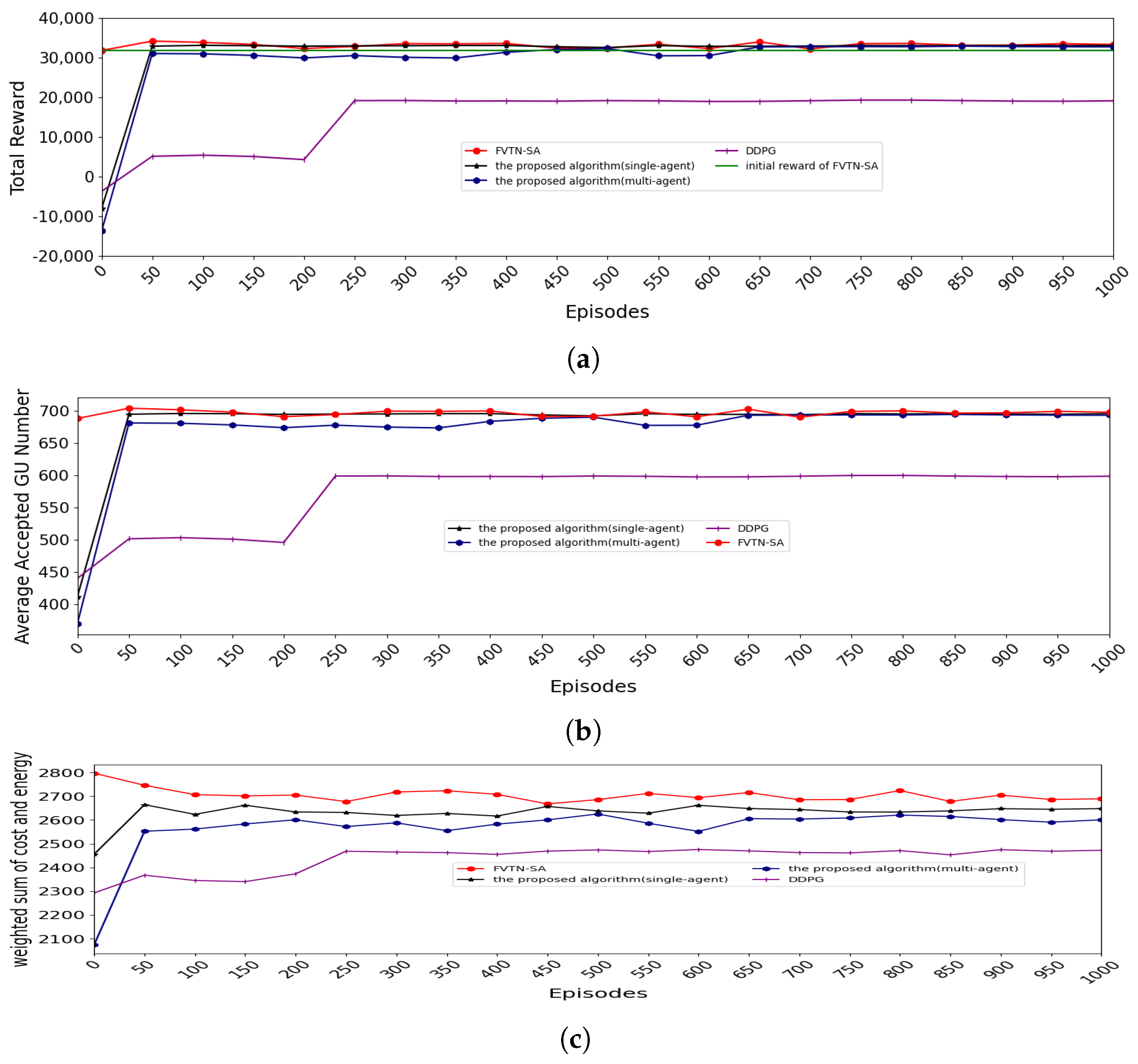
5.1. Convergence of Training Neural Networks

To verify the convergence of the training neural networks in our proposed algorithms (in the single- and multi-agent cases) and DDPG, where the three algorithms were used to solve the proposed problem, we stored the trained neural networks’ models every 50 episodes. To facilitate testing, a test state $Test\_stat{e}_1$ with 15 GUs and their locations and requests in each time frame was generated.

The Online-VNF-Qnetwork and the UAVs-Trajectories Actor Network were the networks used to generate discrete actions and continuous actions, respectively. Thus, the fixed VNF deployments during the entire T were obtained using GTMTVT, and the UAV trajectories were obtained using the UAVs-Trajectories Actor Network in the single-agent case. FVTN-SA was used to test the convergence of the UAVs-Trajectories Actor Network in the single-agent case. Regarding the convergence of the Online-VNF-Qnetwork and the whole training process in the single-agent case obtained using the proposed (single-agent) algorithm, all test results are shown in Figure 4. The results (total reward) were averaged from 50 tests on $Test\_stat{e}_1$.

Figure 4a shows that the initial reward of FVTN-SA is large. The two reasons for this are as follows: the used VNF deployments are preferable, and the action execution process decides that the narrowed UAV flight selection area is the area that is close to or even belongs to the best result under the corresponding deployment. Because the rewards were large numbers, when we looked at the convergence of the UAVs-Trajectories Actor Network in the single-agent case, we checked whether the fluctuation decreased. Looking at the line for FVTN-SA, because all rewards obtained by the trained UAVs-Trajectories Actor Network were larger than the initial reward, the training was effective. From 750 episodes, the reduction in volatility was found to be a nearly straight line. Therefore, the training of UAVs-Trajectories Actor Network converged at 750. Figure 4a shows that our proposed algorithms (in the single- and multi-agent cases) and DDPG all converged from 750 episodes, as evidenced by their decreased fluctuation. Thus, in later training, we set training episodes to 1000. In general, on the basis of mapping discrete variables to continuous variables and using the DDPG method to solve the problem, oscillation occurs at convergence. However, our modified DDPG algorithm used for comparison converged well. This may be because our method of mapping discrete variables to continuous variables is a value mapping (i.e., all VNF deployments on a UAV are regarded as a continuous variable, then VNF deployment on a UAV is obtained according to the value of the continuous variable), rather than probabilistic selection (each VNF deployment on a UAV has a continuous variable representing its possibility; then, for a UAV, the VNF deployment with the highest continuous variable/probability is selected).

Figure 4a also shows that our proposed algorithms (for both the single- and the multi-agent cases) are better than DDPG. This is probably because using the value mapping method to map the discrete variable to the continuous variable results in local optimality. Specifically, the continuous value ranges on the sides of the continuous values’ range, representing better VNF deployment, may represent poor VNF deployments. Assigning value ranges to VNF deployments by ranking the VNF deployments from good to bad is impossible because VNF deployment being good or bad differs for different states or even for different time frames in the same states. (For example, the best VNF deployment 1 for state 1 may be a worse or even the worst VNF deployment for state 2.) Therefore, the use of DDPG to solve the proposed problems has many shortcomings, and our proposed algorithms (for both the single- and multi-agent cases) are effective and show promise. We conducted many training rounds, and the convergence was similar to that shown in Figure 4a. However, sometimes, the convergence result was not ideal because of a problem with training sample selection (samples were all randomly selected). The results of repeated training using these three methods were as follows: each method was trained six times (the training samples for each training were randomly generated and different). The proposed algorithm (the single-agent case) converged five times in a situation similar to that shown in Figure 4; the proposed algorithm (the multi-agent case) converged four times following the situation shown in Figure 4; DDPG only converged following the situation shown in Figure 4 twice. The rest of the training results were worse than those in Figure 4. Thus, the dependence of the proposed algorithms (the single- and multi-agent cases) and DDPG on the selection of training samples, from low to high, is the proposed algorithm (single-agent case), the proposed algorithm (multi-agent case), and DDPG. Therefore, in future work, we will study the design of training samples to ensure good training results. In the following tests, the neural network models, including the proposed algorithms (the single- and multi-agent cases) and DDPG, as shown after many training rounds for testing, all converged to better results.

Figure 4a shows that the total reward was a very large number when we set $Coe{f}_1^P$ to a large constant. The problem target factually consists of two subtargets (the accepted number of requests and the weighted sum of cost and energy consumption). Thus, to more clearly see the target and compare the results, the accepted number of requests and the weighted sum of cost and energy consumption are shown instead of the total reward (target calculated using Equation (31)). On this basis, we separately examined convergence from the perspective of these two indicators by testing on $Test\_stat{e}_1$, with the results shown in Figure 4b,c.

Figure 4b is similar to Figure 4a. Through training, the accepted number of requests of the three algorithms, which were the proposed algorithms (single- and multi-agent) and DDPG, increased. They also maintained stability at the end of the epochs; that is, they converged. For FVTN-SA, the average number of accepted requests fluctuated less, which means the UAVs-Trajectories Actor Network in the single-agent case converged. However, the performance of the DDPG algorithm was worse than that of our proposed algorithms (in both the single- and multi-agent cases). The reasons for these results are also the same as those provided for the results in Figure 4a.

Figure 4c shows that through training, all algorithms converged. For FVTN-SA, the weighted sum of cost and energy decreased. This is because the VNF deployment for FVTN-SA was the deployment scheme that could accept as many requests as possible; in this case, we observed that, by training, the UAVs-Trajectories Actor Network made the weighted sum of cost and energy larger when the accepted request number was already larger. The result showed that the training of UAVs-Trajectories Actor Network achieved this goal. As for the other three algorithms, their weighted sums increased because their accepted number of requests increased.

To summarize, from the above analysis of Figure 4, compared with the proposed algorithms (for both the single- and multi-agent cases), the scheme obtained using the existing DDPG algorithm is unsuitable. Therefore, the proposed algorithm is necessary and effective.

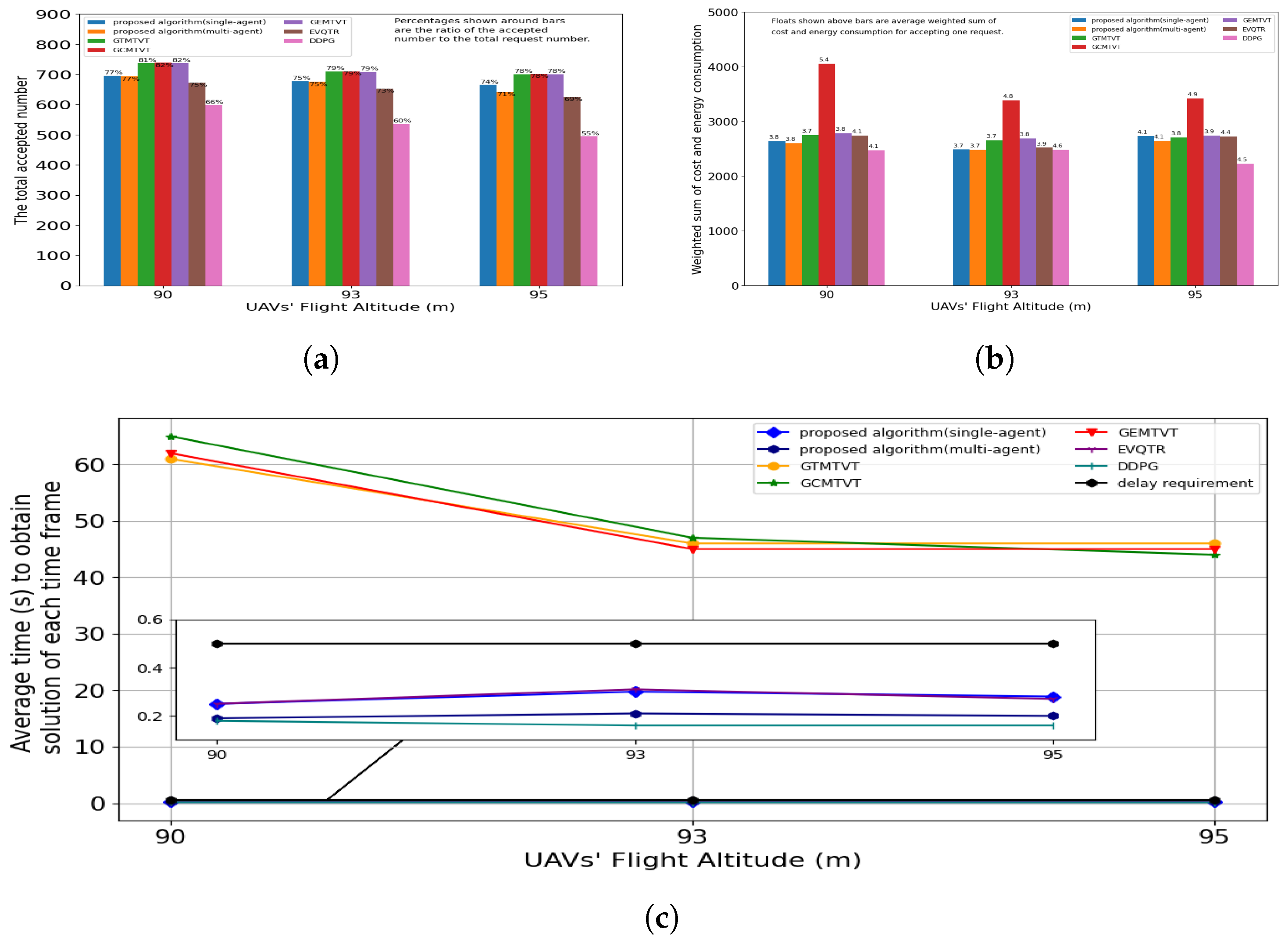
5.2. The Influence of UAV Flight Altitude

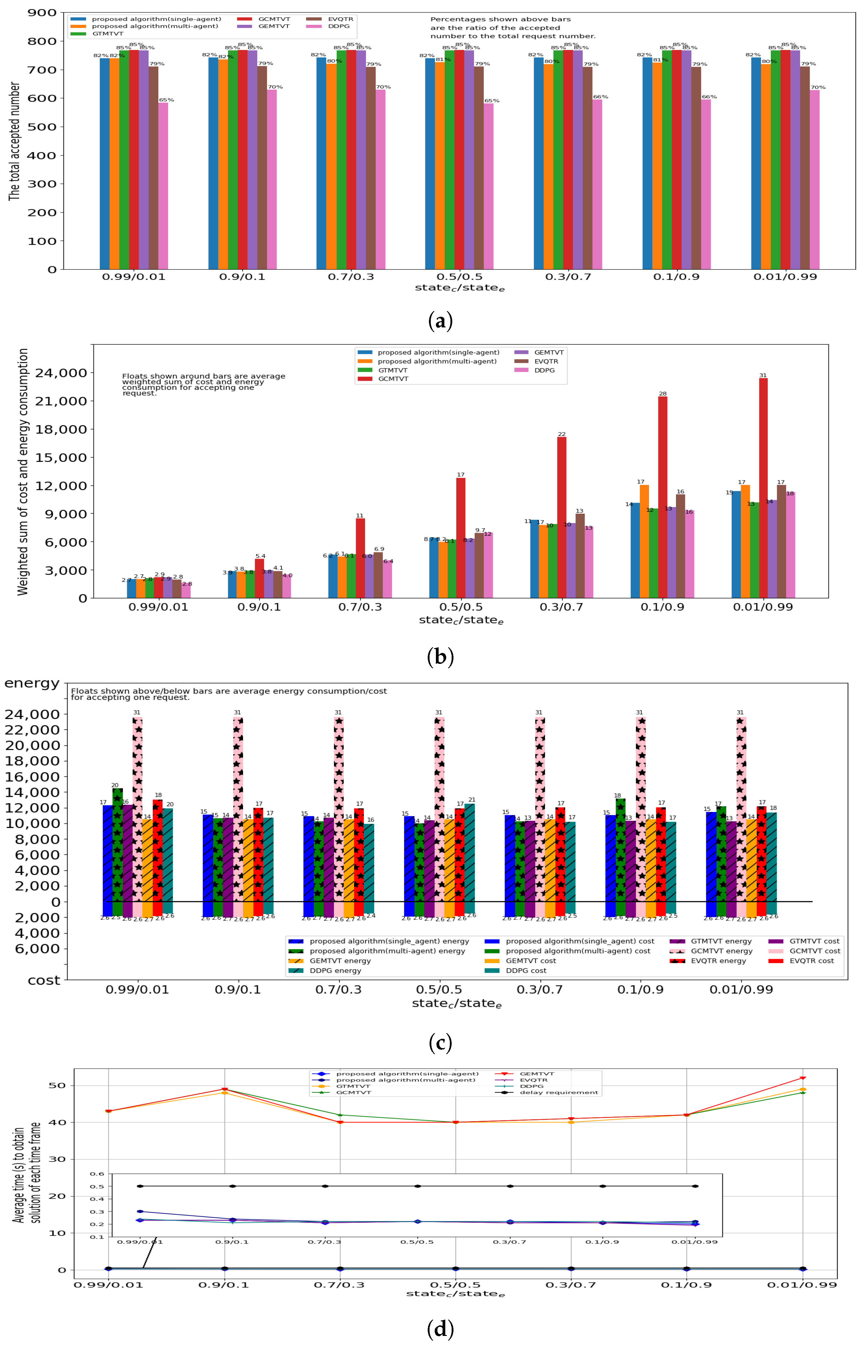
We explored three situations in which the UAVs flew at altitudes of 90, 93, or 95 m. The results averaged from 50 tests on $Test\_stat{e}_1$ are shown in Figure 5. Figure 5a shows that as the flight altitude increased, the accepted number of requests and the acceptance rate (acceptance rate = the accepted number of requests/the total requests number) decreased. This may have occurred because the communication radius of the UAVs mapped to the ground decreased with the increase in flight altitude. Thus, the number of GUs covered by the UAV communication range decreased, leading to a decrease in the accepted number of requests (the acceptance rate).

Figure 5a shows that the acceptance rates of GTMTVT, GCMTVT, and GEMTVT were basically the same, which can be regarded as the best. The acceptance rate of our proposed algorithm (the single-agent case) was approximately 4% lower than that of these three baselines, which produced the higher acceptance rates. For the proposed algorithm in the multi-agent case, when the altitude was 90 or 93 m, the acceptance rate was basically the same as that of the proposed algorithm in the single-agent case. When the altitude was 95 m, the acceptance rate was approximately 3% less than that of the proposed algorithm in the single-agent case and approximately 7% less than that of these three baselines, which produced the highest acceptance rates. This may have occurred because the higher the altitude, the less communication coverage the UAVs map to the ground, and the stricter requirement for cooperation between UAVs (which is decided by the selected actions) to ensure that more requests are accepted. For the proposed algorithms, the actions generated by the single-agent case cooperated better than those generated by the multi-agent case. This is because the agent in the single-agent case can generate and criticize all actions, whereas an agent in the multi-agent case can only generate and criticize actions related to its corresponding UAV actions. Additionally, the acceptance rates of the five above-mentioned algorithms are higher than those of EVQTR and DDPG. Here, the acceptance rate of DDPG was the lowest among all algorithms. Thus, the acceptance rate of EVQTR was lower than that of the proposed algorithm in the single-agent case, proving that the training of the UAVs-Trajectories Actor Network is important and efficient. The comparison of the results showing that the acceptance rate of DDPG was the lowest proves that the proposed algorithms (in both the single- and multi-agent cases) are necessary and effective.

Our proposed problem is a real-time problem, so the problem needs to be quickly solved. Thus, we evaluated the solutions in terms of the time required to solve the problem, with results shown in Figure 5c. The average time needed for the three baselines (GTMTVT, GCMTVT, and GEMTVT) to obtain the solution in each time frame was at least 80 times larger than the delay requirement, which is unacceptable for real-time problems. The solving time of our proposed algorithms (the single- and multi-agent case) is within the delay limit, and adding solving time is tolerable in some cases compared with the three baselines. Even if our acceptance rate is 4% less than in the results in Figure 5a (in one situation, the acceptance rate was 7% less), compared with the three baselines (GTMTVT, GCMTVT, and GEMTVT), this difference is acceptable under real-time conditions. The acceptance rates of the proposed algorithms (the single- and multi-agent cases) are higher than those of EVQTR, and their test times are similar. For DDPG, although its test time is slightly faster than ours, its acceptance rate is much lower than that of our algorithms, so our algorithms are better than DDPG.

As shown in Figure 5b, GTMTVT’s weighted sum of cost and energy consumption is smaller than that of GCMTVT and GEMTVT. This illustrates the importance of jointly optimizing trajectory planning and VNF deployment. The weighted sums of the proposed problems (for both the single- and multi-agent cases) are smaller than those of GTMTVT, GCMTVT, and GEMTVT; the weighted sum of DDPG is the smallest. However, these may be related to the accepted number of requests. Thus, we examined the average weighted sum for accepting one request. The average weighted sum for GTMTVT was always the smallest. The average weighted sums of our algorithms (both the single- and multi-agent cases) were 0.3 more than that of GTMTVT in the worst case, which is acceptable in consideration of real-time requirements. Additionally, the average weighted sums of both our algorithms were better (less) than that of DDPG, which shows that our algorithms are necessary and effective. Regardless of the accepted number of requests or the weighted sum, the results of our algorithm (the single-agent) are better than EVQTR, indicating that the training of the UAVs-Trajectories Actor Network was effective.

Therefore, from the results in this subsection, we concluded that both our algorithms (the single- and multi-agent cases) are feasible regardless of altitude changes.

5.3. The Influences of ${\omega }_c$ and ${\omega }_e$

A new test state $Test\_stat{e}_2$ with 15 GUs and their locations and requests in each time frame was generated to test the influences of ${\omega }_c$ and ${\omega }_e$. The result, which was averaged from 50 tests, is shown in Figure 6.

Figure 6a shows that with changes in ${\omega }_c$ and ${\omega }_e$, the accepted number of requests (the acceptance rates) in the problem solution obtained by GTMTVT, GCMTVT, and GEMTVT did not change. This is because ${\omega }_c$ and ${\omega }_e$ are parameters related to the second-priority goal (minimizing the weighted sum of costs and energy consumption) and are unrelated to the first-priority goal (maximizing the number of requests). Thus, we found that one of the metrics used to judge the algorithms provided a relatively good method to solve the proposed problem: the accepted number of requests (the acceptance rate) did not considerably fluctuate with changes in ${\omega }_c$ and ${\omega }_e$. From Figure 6a, we find that the accepted number of requests obtained by the proposed algorithm (the single-agent case) and EVQTR only have a small fluctuation with changing ${\omega }_c$ and ${\omega }_e$, and their small fluctuations cannot even be seen from the acceptance rate we give. The accepted number of requests obtained using the proposed algorithm in the multi-agent case fluctuated slightly more than in the single-agent case with changes in ${\omega }_c$ and ${\omega }_e$. Specifically, the acceptance rate in the multi-agent case fluctuated around 2%. This may have occurred because the proposed algorithm for the single-agent case is less dependent on training sample selection than that of the multi-agent case. Therefore, the proposed algorithm for the single-agent case more easily converged to the same value, whereas the final convergence values of the multi-agent case showed a certain deviation. DDPG produced the largest fluctuation in the number of requests among all methods when ${\omega }_c$ and ${\omega }_e$ change. This is because DDPG strongly depends on training sample selection, which leads to its final convergence values showing large deviation.

Figure 6a also shows that the acceptance rates of GTMTVT, GCMTVT, and GEMTVT are basically the same, which can be regarded as the highest. The acceptance rate of our proposed algorithm (the single-agent case) is approximately 3% less than that of these three baselines. The other proposed algorithm for the multi-agent case has an acceptance rate of approximately 2% less in the worst case than that in the single-agent case. This is because the agent in the single-agent case can always consider all actions, whereas an agent in the multi-agent case can only focus on actions related to its corresponding UAVs’ actions. This further leads to worse cooperation among the actions generated in the multiple-agent case than in the single-agent case. The acceptance rates in the single-agent case are always higher than those of EVQTR, which means the training of the UAVs-Trajectories Actor Network in the single-agent case is important and efficient. Regardless of how ${\omega }_c$ and ${\omega }_e$ change, the acceptance rates of DDPG are the lowest among all considered algorithms. This indicated that both proposed algorithms are necessary and effective.

${\omega }_c$ and ${\omega }_e$ are related to the second-priority metric (the weighted sum of energy consumption and cost); thus, we produced the results shown in Figure 6b. Specifically, with the increase in ${\omega }_e$, the weighted sum increased. The reason can be seen in Figure 6c: the actual energy consumption was several times the actual cost. Additionally, Figure 6c shows that when using GCMTVT or GEMTVT to obtain the solution, the actual energy consumption and cost did not change, regardless of the weight. This is because GCMTVT and GEMTVT pursue the minimum cost/energy consumption, so the weights do not influence their choice. GCMTVT/GEMTVT’s pursuit of cost/energy minimization alone leads to a large energy/cost solution. Thus, the weighted sum of GCMTVT/GEMTVT is greater than that of GTMTVT. For GTMTVT, the actual energy consumption trended downward with the increase in ${\omega }_e$. For both the proposed algorithms and DDPG, the actual energy consumption first trended downward and then stabilized.

The proportions of actual energy consumption and actual cost with changes in ${\omega }_c$/${\omega }_e$ are shown in Figure 7. With increasing ${\omega }_e$, the proportion of actual energy consumption first trended downward and then showed an acceptable state of fluctuation. We inferred that for GTMTVT, this fluctuation occurred when ${\omega }_c$/${\omega }_e$ = 0.01/0.99; its actual energy consumption and proportion of actual energy consumption were both more than those when ${\omega }_c$/${\omega }_e$ = 0.3/0.7 and ${\omega }_c$/${\omega }_e$ = 0.7/0.3. This may be because, in the previous time frames, the optimal weighted sum in the single time frame is excessively pursued when guaranteeing the accepted number of requests. Then, in the later time frames, more weighted sums are needed to maximize the accepted number of requests. The fluctuation in the other three algorithms shown in Figure 7 occurred because of the randomness always present in the selection of continuous variables (trajectories). Thus, the obtained trajectories are not fixed/optimal trajectories: trajectories are always randomly obtained based on the optimal trajectories. This means that the actual energy consumption fluctuates due to the randomness of the trajectory selection (flight energy consumption is related to the trajectories) when using the proposed algorithm. When ${\omega }_e$ is small enough, minimizing cost is the primary goal, and the decision to appropriately increase the energy consumption is made to decrease the cost and thus decrease the weighted sum. Thus, the energy consumption/trajectories choice to obtain the best weighted sum may include a wide range of values, and then energy consumption fluctuations caused by the proposed algorithm can be ignored. By appropriately increasing ${\omega }_e$ at this time, the energy consumption can be reduced as much as possible (that is, to obtain the best weighted sum, the selection range of energy consumption/trajectories is reduced), and the ratio can be reduced. When ${\omega }_e$ increases to a certain value, reducing energy consumption becomes the primary goal. To obtain the best weighted sum, the selection range of energy consumption/trajectories becomes very small. At this time, the energy consumption fluctuations caused by the proposed algorithm are highlighted and cannot be avoided. Thus, when ${\omega }_e$ is increased at this time, the energy consumption fluctuations are always caused by the proposed algorithm. Therefore, as ${\omega }_e$ increases, the ratio fluctuates.

Next, we evaluated the solving time metric, with the results shown in Figure 6d. This metric is crucial for real-time problems. The solving time for GTMTVT, GCMTVT, and GEMTVT to obtain the solution in each time frame was at least 80 times larger than the delay requirement, which is unacceptable for real-time problems. The solving times of our proposed algorithms (both the single- and multi-agent cases) are within the delay limits, and adding solving time is tolerable in some cases compared with that of the three baselines. Even if our acceptance rates and the weighted sums are worse than those of the three baselines, this difference in real-time conditions is acceptable. The acceptance rates of the proposed algorithms (the single- and multi-agent cases) are higher than that of EVQTR, and their test times are similar. Although the DDPG test time is slightly faster than ours, its acceptance rate is too low compared with that of our algorithms, so our algorithms are better than DDPG.

Therefore, from the results in this subsection, we found that both our algorithms are feasible even when the weights change.

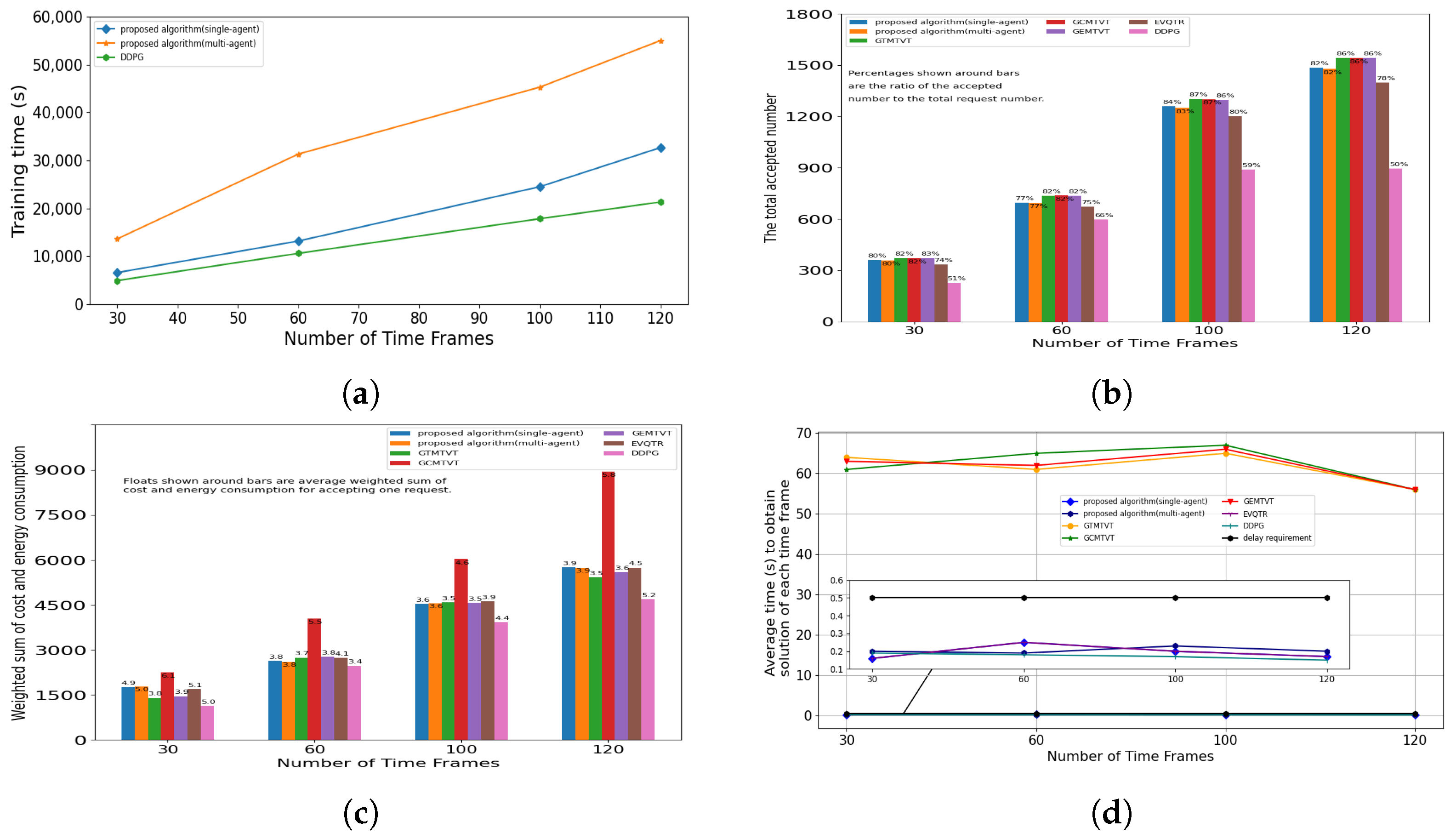
5.4. The Influence of the Number of Time Frames

We set the number of time frames T to 30, 60, 100, and 120. On this basis, test states $Test\_stat{e}_3$ with 30 time frames, $Test\_stat{e}_4$ with 100 time frames, and $Test\_stat{e}_5$ with 120 time frames were generated. For the test state with 60 time frames, we use $Test\_stat{e}_1$. The results are shown in Figure 8.

Figure 8a shows that the training time increased as the number of time frames increased. Before we discuss the reason, note that the DDPG training process is similar to that of Algorithm 1, but DDPG lacks the neural network for obtaining discrete actions because of the discrete actions having been mapped to continuous actions. We can see from the pseudo-code and computational complexity of Algorithms 1 and 2 that their times for the inner loop are related to the number of time frames. On this basis, the higher the number of time frames, the larger the number of inner loops, and thus the longer the training time. The training time of the three algorithms, from short to long, was DDPG, the proposed single-agent algorithm, and the proposed multi-agent algorithm. This is because DDPG only needs to sequentially use/train two kinds of neural networks; the proposed single-agent algorithm needs to sequentially use/train three kinds of neural networks, and the proposed multi-agent algorithm sequentially uses/trains 2 (the number of UAVs set in our simulations)·3 kinds of neural networks in the simulation. When using the proposed multi-agent algorithm, each agent, which involves three kinds of neural networks, can be separately trained, so the training time may be shorter than that provided in the results here.

Figure 8b,c show that the total accepted number of requests and the weighted sum of cost and energy consumption during the whole period that T increased. This occurred because when the GUs number did not change and each GU generated a request in each time frame, the total number of requests substantially increased with large increases in the number of time frames in our test. This led to the total accepted number of requests increasing. The acceptance rates and the weighted sum of cost and energy consumption in accepting each request depend on the GU location and request, so they differ under different test states. Next, we specifically examined the results for each approach. From Figure 8b, the acceptance rates of GTMTVT, GCMTVT, and GEMTVT are basically the same and can be regarded as the highest. For our proposed single-agent and multi-agent algorithms, their acceptance rates were approximately 4% less than those of GTMTVT, GCMTVT, and GEMTV in the worst case. Additionally, regardless of changes in the number of time frames, the acceptance rate of the proposed single-agent algorithm is always higher than that of EVQTR, and DDPG is always the worst method. These two results demonstrate the effectiveness of the training of the UAVs-Trajectories Actor Network and the importance and effectiveness of our proposed algorithms.

Figure 8c also shows that the average weighted sum for accepting each request for GTMTVT is always the best, which proves the importance of jointly optimizing VNF deployment and UAV trajectories. As for our proposed algorithms, their weighted sums for accepting each request are basically approximately 0.4 more than that of GTMTVT and are worse only when the number of time frames is 30. Their average weighted sum is approximately 1.2 more than that of DDPG. However, the average weighted sums of our proposed algorithms are always better than those of EVQTR and DDPG, again proving the importance and effectiveness of our proposed algorithms.

Regarding the most important metric when solving real-time problems, the average time to obtain the solution in each time frame is shown in Figure 8d. The average time did not dramatically change for any algorithm with changes in the number of time frames. The average time of the proposed algorithms, EVTQR, and DDPG, are similar and less than the delay limit, which is acceptable for some real-time problems. The average test time of the other three baselines was more than 55 s, which is far longer than the time frame length (delay requirement) and is unacceptable for real-time problems. Therefore, from the comparison of the above three metrics (the total accepted number, the weighted sum of cost and energy consumption, and the average test time), the proposed algorithms are feasible for any number of time frames.

Additionally, we further analyzed the reason why the total weighted sums of GTMTVT and GEMTVT were better than those of GCMTVT, and why those of the proposed algorithms were better than those of EVQTR. We did not consider DDPG in this analysis because the accepted number of requests by DDPG was much smaller than that of other algorithms. We started analyzing the reason for this finding using

Table 2. Actual cost and actual energy in each time frame testing on $Test\_stat{e}_3$ using GTMTVT, GCMTVT, and GEMTVT.

Time Frame	GTMTVT		GCMTVT		GEMTVT
	Cost	Energy	Cost	Energy	Cost	Energy
1	24.137	135.174	23.975	552.144	24.137	135.174
2	36.176	849.687	35.258	235.078	36.176	849.687
3	34.879	431.842	34.879	431.842	34.879	431.842
4	32.585	105.844	30.761	248.601	32.585	105.844
5	30.434	105.858	28.051	321.329	30.434	105.858
6	37.77	111.725	36.04	692.163	37.77	111.725
7	36.054	105.862	35.629	205.579	36.054	105.862
8	41.046	278.293	35.647	105.895	41.046	278.293
9	33.567	105.891	36.235	523.825	33.567	105.891
10	34.992	211.455	34.992	250.411	34.992	211.455
11	36.128	105.925	35.592	647.442	40.56	105.887
12	34.517	105.93	33.595	820.811	35.441	105.908
13	37.946	105.974	37.946	105.974	38.865	105.974
14	30.729	105.886	35.092	461.745	35.092	211.418
15	29.339	105.895	29.82	523.491	31.302	105.868
16	34.434	105.966	32.412	552.579	35.443	141.444
17	34.372	321.456	32.307	531.635	34.372	226.539
18	34.807	105.928	33.15	105.9	35.236	105.899
19	40.634	105.934	37.478	150.738	40.634	105.934
20	30.341	111.768	29.477	692.16	30.341	111.768
21	37.73	105.933	36.812	105.933	37.73	105.933
22	35.437	105.964	32.465	529.671	35.437	105.964
23	34.641	105.927	33.086	461.745	34.641	105.927
24	42.589	180.398	41.877	351.109	45.19	180.396
25	33.813	644.433	33.813	321.477	33.813	644.433
26	33.481	105.905	33.481	226.5	34.394	105.862
27	36.197	105.902	34.95	182.539	37.301	105.902
28	32.211	211.412	29.52	205.611	32.471	211.424
29	34.606	135.475	29.19	205.458	31.218	105.836
30	36.462	105.948	36.513	736.994	38.484	105.948

and

Table 3. Actual cost and actual energy in each time frame testing on $Test\_stat{e}_3$ using the proposed algorithms and EVQTR.

Time Frame	Proposed Algorithm (Single-Agent)		Proposed Algorithm (Multi-Agent)		EVQTR
	Cost	Energy	Cost	Energy	Cost	Energy
1	24.53	252.85	20.96	549.29	23.84	282.43
2	27.98	785.8	29.08	550.13	25.66	652.17
3	32.08	633.47	32.06	621.75	30.92	414.01
4	30.97	468.07	30.73	443.12	28.84	510.56
5	32.76	147.67	33.09	117.75	30.7	245.18
6	36.51	423.64	37.46	449.6	32.69	266.49
7	32.85	280.99	32.4	221.53	32.63	266.35
8	38.02	426.19	38.63	461.57	32.02	316.94
9	32.78	608.22	32.95	716.55	30.9	409.1
10	35.37	196.54	35.03	210.32	32.23	235.8
11	32.29	425.12	32.37	397.17	30.2	438.39
12	33.27	214.26	33.34	238.74	32.3	317.13
13	35.04	139.68	34.85	149.16	32.33	160.84
14	33.99	116.48	33.99	116.16	31.88	200.15
15	31.69	282.69	31.52	259.51	29.68	245.5
16	32.19	107.81	32.23	108.37	29.98	118.15
17	30.7	166.63	30.52	131.62	30.38	196.0
18	34.2	450.28	34.4	512.75	31.97	378.7
19	36.8	144.01	36.79	147.74	35.15	170.51
20	31.67	152.83	31.54	154.16	29.01	187.53
21	32.03	161.32	32.02	169.25	29.58	270.04
22	32.51	122.1	32.49	129.18	30.79	256.44
23	28.54	556.23	28.52	544.3	26.11	385.01
24	33.82	251.33	33.79	283.2	32.14	230.87
25	31.01	125.78	30.82	131.34	29.49	133.21
26	34.25	192.43	34.47	157.7	31.97	414.36
27	30.79	107.21	30.44	107.21	30.08	161.38
28	31.19	166.53	31.16	233.18	28.38	216.46
29	30.97	527.64	31.14	572.12	29.27	314.18
30	35.42	240.78	35.52	236.78	33.86	377.48

, for which the results were averaged by testing on $Test\_stat{e}_3$ 50 times. The two tables show that the total weighted sums of GTMTVT and GEMTVT were mainly due to consuming less energy than GCMTVT, and the same was applied to the difference between the proposed algorithms and EVQTR. Energy consumption is mostly related to flight velocity (trajectories) based on Equation (24). Thus, by using $Test\_stat{e}_3$, the trajectories generated by GTMTVT, GEMTVT, and GCMTVT are compared in Figure 9a, and the trajectories generated by the proposed algorithms and EVQTR are compared in Figure 9b. We chose the best results from 50 tests.

Before explaining the comparison shown in Figure 9, based on Equation (21) and simulation parameters, we must point out that when the UAV was flying at a velocity of 10.4 m/s (the flight distance was 5.2 m because the time frame length was 0.5 s), the flight energy consumption for a time frame was the lowest. When the flight velocity was less than 10.4 m/s, the slower the flight velocity, the larger the energy consumption. When the flight velocity was more than 10.4 m/s, (1) the higher the flight velocity, the higher the energy consumption, and (2) the higher the velocity, the greater the energy consumption to increase the unit speed. Figure 9a shows that in the trajectories generated by GTMTVT/GEMTVT, UAVs fly with the velocity that produces the lowest energy consumption possible. However, GCMTVT seeks to minimize costs, so if it wants to accept as many requests as possible, UAVs may need to fly at a velocity at which the energy consumption is high to visit the corresponding GUs. By comparing the trajectories generated by the proposed single-agent and multi-agent algorithms and EVQTR in Figure 9b, we found that training leads to the UAVs visiting the corresponding GUs at the velocity with the lowest energy consumption.

Therefore, from the results in this subsection, we found that our algorithms are feasible even when the UAV velocity changes.

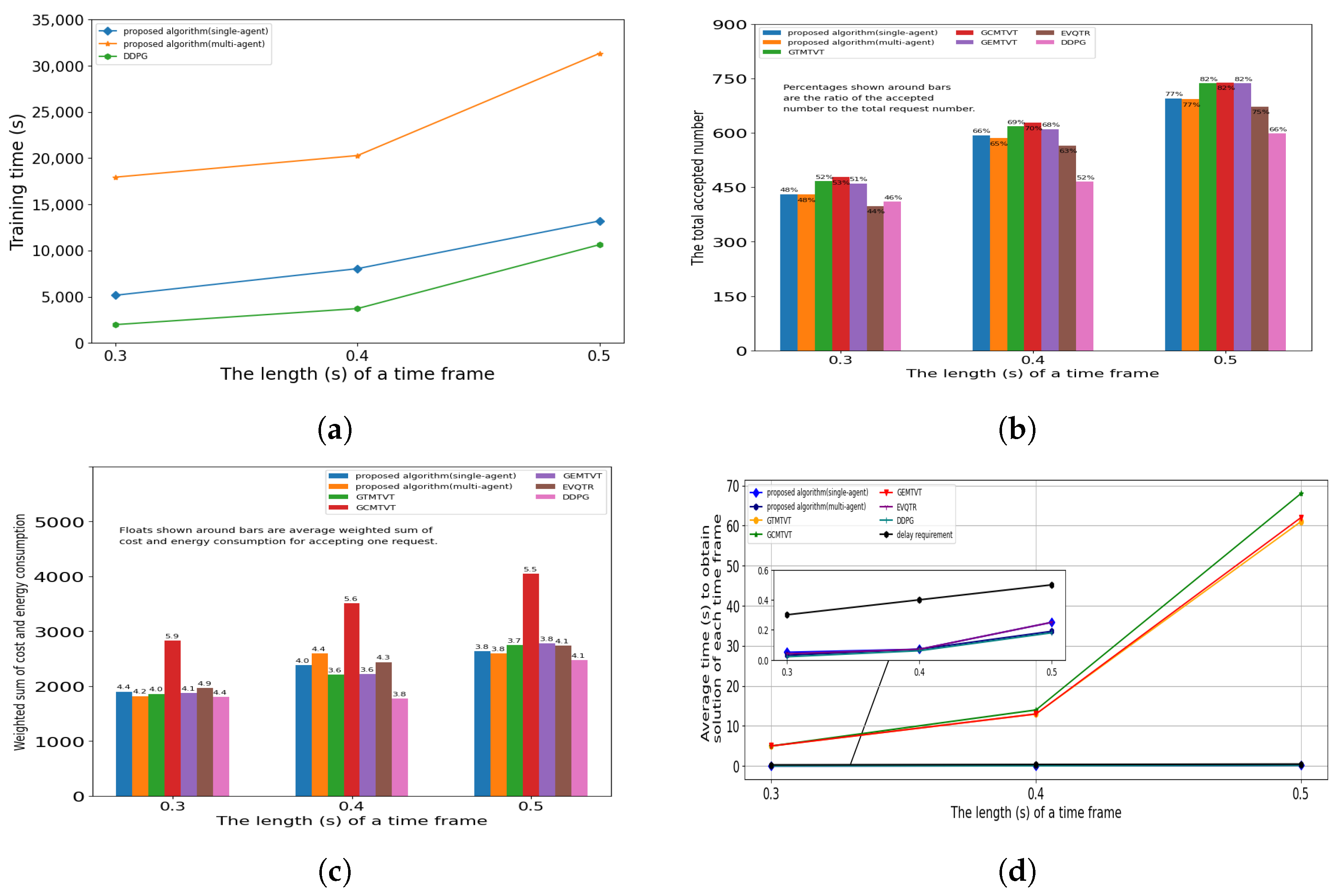
5.5. The Influence of Time Frame Length

The time delay requirements of real-time problems are relatively strict, so we set 0.3 s, 0.4 s, and 0.5 s as three time delays (time frame length) in this study. We used test states $Test\_stat{e}_6$ with a time frame length of 0.3 s and $Test\_stat{e}_7$ with a time frame length of 0.4 s. For the test state with the time frame length of 0.5 s, we use $Test\_stat{e}_1$. The result is shown in Figure 10.

For all three algorithms shown in Figure 10a, the longer the time frame length, the longer the training time. Notably, for these three algorithms, their action-execution processes are the same, which was explained in the Action-Selection and Execution Process section for the single-agent centralized scenario. The longer each time frame’s length, the further the maximum flying distance of a UAV. We fixed $l_{grid}$; here, the longer each time frame’s length, the larger the number of grid nodes $N_{node}$, further leading to more combinations $N_{node}^M$ of all mobile UAVs. From the Action-Selection and Execution Process section, we know that $N_{node}^M$ is the number needed to be traversed for determining the flying range. Thus, the training time increases with the increasing length of the time frame.

In Figure 10b, for all algorithms, the accepted number of requests (acceptance rate) increases as the time frame lengthens. The two possible reasons for this are as follows. First, as the flying range of the UAVs increases, they can choose locations that can accept more requests. Second, the increase in the time frame length increases the UAVs’ available computing resources in one time frame. Thus, UAVs can process more requests in one time frame. The weighted sum of energy consumption and cost shown in Figure 10c increases for all algorithms for two reasons. One is that even flying at the same velocity, the longer the flight time, the greater the energy consumption. The other is that processing more requests increases computational cost and consumption. As the average weighted sum for accepting one request decreases, the average weighted sums for five algorithms (the proposed algorithm for the single-agent case, GTMTVT, GCMTVT, and GEMTVT) decrease. This is due to the increasing proportion of the total weighted sum being less than that of the accepted request number. The average weighted sum of accepting one request for the proposed multi-agent algorithm and DDPG fluctuates. This is because the actions generated by the proposed algorithm (multi-agent) cooperate worse than the actions generated in the multiple-agent case, and the training results of DDPG are strongly dependent on the training samples. The average time to obtain the solution for each time frame shown in Figure 10d increases because the combinations $N_{node}^M$ of all mobile UAVs that need to be traversed increase.

Figure 10b compares the proposed algorithms (the single- and multi-agent cases) with the baselines in terms of acceptance rate: that of the proposed algorithm is 5% less than that of GTMTVT, GCMTVT, and GEMTVT but is always better than that of EVQTR and DDPG. This shows the importance and effectiveness of the proposed algorithms. The weighted sum accepting one request shown in Figure 10c for the proposed single-agent algorithm is 0.4 more than that of GTMTVT, whose weighted sum for accepting one request is the lowest, but it is always better than that of EVQTR. The proposed multi-agent algorithm has a weighted sum for accepting one request that is 0.8 more than that of GTMTVT when the time frame length is 0.4s, whereas, for the other two time-frame length cases, its weighted sum for accepting one request is 0.1/0.2 more than that of GTMTVT. This may be caused by the training sample selection when training the proposed multi-agent algorithm.

Figure 10d shows the average solution time in one time frame for the proposed algorithms. Those of EVQTR and DDPG are similar, and their average solution time in one time frame is acceptable for the real-time problem. The average solution time in one time frame of the other three baselines is many times larger than the delay requirement, which is unacceptable for real-time problems.

From the above analysis, we found that the proposed algorithm is feasible even as the time frame length decreases.

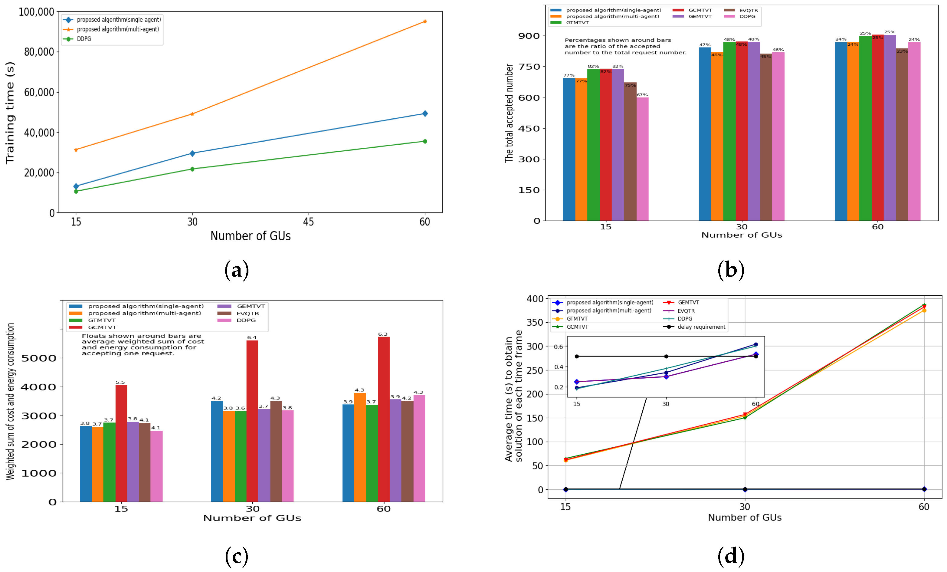
5.6. The Influence of GU Number

We set the number of GUs K to 15, 30, and 60. On this basis, test states $Test\_stat{e}_8$ with 30 GUs and $Test\_stat{e}_9$ with 60 GUs were generated. For the test state with 15 GUs, we used $Test\_stat{e}_1$. When K = 30, in the single-agent case, the VNF-Q-Network had a hidden layer with 64 neurons; the hidden layers of the Trajectory Actor Network had [128, 32, 8] neurons; the hidden layers of the Critic Network had [64, 16, 2] neurons; in the multi-agent case, the hidden layers of the VNF-Q-Network m(m∈$\mathcal{M}$) had [64, 16] neurons; the hidden layers of the Trajectory Actor Network m had [64, 16, 4] neurons; and the hidden layers in the Critic Network m had [64, 16, 2] neurons. For DDPG, the hidden layers of its actor network had [128, 32, 8] neurons, and the hidden layers of its critic network had [64, 16, 2] neurons. When K = 60, in the single-agent case, the VNF-Q-Network had a hidden layer with 128 neurons; the hidden layers of the trajectory Actor Network had [128, 64, 16] neurons; and the hidden layers of the Critic Network had [128, 32, 2] neurons. In the multi-agent case, the hidden layers of the VNF-Q-Network m(m∈$\mathcal{M}$) had [128, 32] neurons; the hidden layers of Trajectory Actor Network m had [128, 32, 8] neurons; the hidden layers of the Critic Network m had [128, 16, 2] neurons. For DDPG, the hidden layers of its actor network had [128, 64, 16] neurons, and the hidden layers of its critic network had [128, 32, 2] neurons. The results are shown in Figure 11.

Figure 11a shows that as the number of GUs increases, the longer the training time required. One reason for this is shown by the results of the computational complexity analyses in the previous section: the number of GUs influences computational complexity. Specifically, the larger the number of GUs, the higher the computational complexity. Another reason is that the number of neurons in the hidden layers increases as the number of GUs increases.

Figure 11b shows that the accepted number of requests increases as the number of GUs increases. This is because the larger the number of GUs, the higher the distribution density. In the case of a fixed UAV communication range, UAVs can visit more GUs with a higher distribution density. Thus, more requests can be accepted. However, as the number of GUs increases, the increase in the accepted number of requests decreases (the acceptance rate decreases). This may occur for two reasons: (1) the available UAV resources are limited in one time frame, and (2) there are GU locations and requests. Additionally, the acceptance rates of GTMTVT, GCMTVT, and GEMTVT remained basically the same and can be regarded as the acceptance rates. The acceptance rates of the proposed algorithms, in the worst case, were approximately 5% less than those of GTMTVT, which had the highest acceptance rate, but they are always better than those of EVQTR. The latter comparison proves the effectiveness of the training the UAVs-Trajectories Actor Network. Figure 11c shows that for the weighted sum of cost and energy consumption of accepting one request, GTMTVT was always the best, which proves the importance of the joint optimization of VNF deployment and UAV trajectories. In addition, our algorithms had weighted sums that were, in the worst case, 0.6 more than that GTMTVT, but they were always better than EVQTR. The average time to obtain the solution in each time frame shown in Figure 11d increases with the increase in GU number. This is because each GU needs to be traversed when determining the request acceptance. Thus, the larger the number GUs, the longer the time needed. In the previous subsection, the test times of the proposed algorithm and EVQTR were shown to be similar and acceptable for some real-time problems. The average solution time for one time frame of GTMTVT, GCMTVT, and GEMTVT is even many times larger than the delay limit, so they are unsuitable for real-time problems. From the above, we found that the proposed algorithms are more feasible when the number of GUs changes within some range than GTMTVT, GCMTVT, GEMTVT, and EVQTR. When the number of GUs number is very large, the average solution time for one time frame of our proposed algorithms may be much longer than the delay limit. Thus, when the number of GUs is large, our proposed algorithm should be further improved, which will be studied in our future work.

Next, we compared the proposed algorithms for both the single- and multi-agent cases with DDPG, as shown in Figure 11. As shown in Figure 11b, with 15 GUs, the accepted number of requests (acceptance rate) of DDPG is much smaller than that of the proposed algorithms. In the other two cases (30 and 60 GUs), the accepted number of requests (acceptance rate) of DDPG is similar to that of the proposed algorithms. This occurs because as the number of GUs increases, the density of the GU distribution and the number of requests requiring the same type of VNF increase, resulting in increased VNF deployment and more UAV-trajectory combinations that can achieve the goal. Therefore, selecting training samples that produce better results is easier, which leads to DDPG obtaining better results. In Figure 11c, the weighted sums of cost and energy consumption of accepting one request for DDPG are similar to those of the proposed algorithms. We present the 50 test results when the number of GUs K is 30 and 60 in more detail in

Table 4. Test results for different numbers of GUs using the proposed algorithms and DDPG.

		Proposed Algorithm (Single Agent)		Proposed Algorithm (Multi-Agent)		DDPG
		K= 30	K= 60	K= 30	K= 60	K= 30	K= 60
Accepted request number	max	849	879	825	883	823	875
	min	831	846	814	860	815	856
	avg	842.88	870.28	819.62	870.78	819.72	868.32
	std	30.55	32.31	14.89	32.78	14.36	24.14
Weighted sum of cost and energy consumption	max	3771.29	3822.59	3344.37	4376.71	3457.33	4019.02
	min	3215.33	3075.34	2980.52	3515.32	2934.55	3317.69
	avg	3489.75	3348.85	3147.99	3808.39	3170.55	3741.01
	std	910.55	1307.24	541.13	1171.01	785.85	1009.55

to compare the proposed algorithms with DDPG. Table 4 shows that when K = 30, the accepted number of requests for the proposed single-agent algorithm is considerably higher than those of the proposed multi-agent algorithm and DDPG. Then, we only needed to compare the proposed algorithm (multi-agent) and DDPG when K = 30. In terms of the number of accepted requests, the performance of the proposed algorithm (multi-agent) and DDPG was similar. Regarding the weighted sum of cost and energy consumption, the proposed algorithm (multi-agent) performed better. When K = 60, the proposed single-agent algorithm and DDPG performed similarly in terms of the accepted number of requests, but the proposed single-agent algorithm performed better in terms of the maximum, minimum, and average of the weighted sum. The proposed multi-agent algorithm performed better than DDPG in terms of the maximum, minimum, and average of the accepted number of requests. Notably, the weighted sum of the proposed multi-agent algorithm can be further optimized.

From the above analysis, we found that the proposed algorithm is promising, although some problems with both our algorithms (single-agent and multi-agent) arise for larger GU numbers.

From the above six aspects of analysis, we found that the design of our algorithms (for the single- and multi-agent cases) is necessary, effective, and promising, because they generally performed well in our simulations. However, some aspects require improvement: (1) Our algorithms can converge to better results, but this is closely related to the selection of training samples. Thus, the selection of training samples needs to be further studied to ensure that the algorithm always converges to an acceptable result. (2) From the perspective of combining multiple metrics (accepted number of requests, the weighted sum of cost and energy consumption, and solving time to obtain real-time problem solutions) to evaluate the algorithms used for real-time problems, our algorithms were better than the baseline algorithms. However, when only considering the accepted number of requests and the weighted sum of cost and energy consumption, our algorithms need to be improved. (3) We need to improve the proposed algorithms to ensure that as the number of GUs grows, the time required to obtain real-time problem solution still meets the latency requirements.

6. Conclusions

In this study, we discussed the online joint optimization of VNF deployment and trajectory planning in multi-UAV mobile-edge networks. Our aim was to maximize the accepted number of requests under a given period T while minimizing both the energy consumption and the cost of accepting the requests for all UAVs with constraints on UAV resources and real-time request latency. To tackle this problem, we designed an online DRL based on jointly optimizing discrete and continuous actions. When we designed the algorithm, we considered both the single- and multi-agent cases. Then, we compared the developed algorithm with some baseline algorithms through simulations to verify that our algorithm is promising. The shortcomings of the proposed algorithms were described. Thus, in future work, we will improve the algorithm’s performance in terms of various aspects, such as through the design of training samples. We can also think about UAV heterogeneity and situations where the UAV altitude changes during flight. In the multi-agent case, we will further consider situations where an agent can only obtain partial information.

References

1. Zhou, F.; Hu, R.Q.; Li, Z.; Wang, Y. Mobile Edge Computing in Unmanned Aerial Vehicle Networks. IEEE Wirel. Commun. 2020, 27, 140–146. [Google Scholar] [CrossRef]
2. Le, L.; Nguyen, T.N.; Suo, K.; He, J.S. 5G network slicing and drone-assisted applications: A deep reinforcement learning approach. In Proceedings of the 5th International ACM Mobicom Workshop on Drone Assisted Wireless Communications for 5G and Beyond, DroneCom 2022, Sydney, NSW, Australia, 17 October 2022; ACM: New York, NY, USA, 2022; pp. 109–114. [Google Scholar] [CrossRef]
3. Nogales, B.; Vidal, I.; Sanchez-Aguero, V.; Valera, F.; Gonzalez, L.; Azcorra, A. OSM PoC 10 Automated Deployment of an IP Telephony Service on UAVs using OSM. In Proceedings of the ETSI-OSM PoC 10, Remote, 30 November–4 December; 2020. Available online: https://dspace.networks.imdea.org/handle/20.500.12761/911 (accessed on 18 January 2024).
4. Quang, P.T.A.; Bradai, A.; Singh, K.D.; Hadjadj-Aoul, Y. Multi-domain non-cooperative VNF-FG embedding: A deep reinforcement learning approach. In Proceedings of the IEEE INFOCOM 2019—IEEE Conference on Computer Communications Workshops (INFOCOM WKSHPS), Paris, France, 29 April–2 May 2019; pp. 886–891. [Google Scholar] [CrossRef]
5. Xu, Z.; Gong, W.; Xia, Q.; Liang, W.; Rana, O.F.; Wu, G. NFV-Enabled IoT Service Provisioning in Mobile Edge Clouds. IEEE Trans. Mob. Comput. 2021, 20, 1892–1906. [Google Scholar] [CrossRef]
6. Ma, Y.; Liang, W.; Li, J.; Jia, X.; Guo, S. Mobility-Aware and Delay-Sensitive Service Provisioning in Mobile Edge-Cloud Networks. IEEE Trans. Mob. Comput. 2022, 21, 196–210. [Google Scholar] [CrossRef]
7. Ma, Y.; Liang, W.; Huang, M.; Xu, W.; Guo, S. Virtual Network Function Service Provisioning in MEC Via Trading Off the Usages Between Computing and Communication Resources. IEEE Trans. Cloud Comput. 2022, 10, 2949–2963. [Google Scholar] [CrossRef]
8. Ren, H.; Xu, Z.; Liang, W.; Xia, Q.; Zhou, P.; Rana, O.F.; Galis, A.; Wu, G. Efficient Algorithms for Delay-Aware NFV-Enabled Multicasting in Mobile Edge Clouds With Resource Sharing. IEEE Trans. Parallel Distrib. Syst. 2020, 31, 2050–2066. [Google Scholar] [CrossRef]
9. Huang, M.; Liang, W.; Shen, X.; Ma, Y.; Kan, H. Reliability-Aware Virtualized Network Function Services Provisioning in Mobile Edge Computing. IEEE Trans. Mob. Comput. 2020, 19, 2699–2713. [Google Scholar] [CrossRef]
10. Yang, S.; Li, F.; Trajanovski, S.; Chen, X.; Wang, Y.; Fu, X. Delay-Aware Virtual Network Function Placement and Routing in Edge Clouds. IEEE Trans. Mob. Comput. 2021, 20, 445–459. [Google Scholar] [CrossRef]
11. Qiu, Y.; Liang, J.; Leung, V.C.M.; Wu, X.; Deng, X. Online Reliability-Enhanced Virtual Network Services Provisioning in Fault-Prone Mobile Edge Cloud. IEEE Trans. Wirel. Commun. 2022, 21, 7299–7313. [Google Scholar] [CrossRef]
12. Li, J.; Liang, W.; Xu, W.; Xu, Z.; Jia, X.; Zomaya, A.Y.; Guo, S. Budget-Aware User Satisfaction Maximization on Service Provisioning in Mobile Edge Computing. IEEE Trans. Mob. Comput. 2022, 22, 7057–7069. [Google Scholar] [CrossRef]
13. Li, J.; Guo, S.; Liang, W.; Chen, Q.; Xu, Z.; Xu, W.; Zomaya, A.Y. Digital Twin-Assisted, SFC-Enabled Service Provisioning in Mobile Edge Computing. IEEE Trans. Mob. Comput. 2022, 23, 393–408. [Google Scholar] [CrossRef]
14. Liang, W.; Ma, Y.; Xu, W.; Xu, Z.; Jia, X.; Zhou, W. Request Reliability Augmentation With Service Function Chain Requirements in Mobile Edge Computing. IEEE Trans. Mob. Comput. 2022, 21, 4541–4554. [Google Scholar] [CrossRef]
15. Tian, F.; Liang, J.; Liu, J. Joint VNF Parallelization and Deployment in Mobile Edge Networks. IEEE Trans. Wirel. Commun. 2023, 22, 8185–8199. [Google Scholar] [CrossRef]
16. Liang, J.; Tian, F. An Online Algorithm for Virtualized Network Function Placement in Mobile Edge Industrial Internet of Things. IEEE Trans. Ind. Inform. 2023, 19, 2496–2507. [Google Scholar] [CrossRef]
17. Wang, X.; Xing, H.; Song, F.; Luo, S.; Dai, P.; Zhao, B. On Jointly Optimizing Partial Offloading and SFC Mapping: A Cooperative Dual-Agent Deep Reinforcement Learning Approach. IEEE Trans. Parallel Distrib. Syst. 2023, 34, 2479–2497. [Google Scholar] [CrossRef]
18. Bai, J.; Chang, X.; Rodríguez, R.J.; Trivedi, K.S.; Li, S. Towards UAV-Based MEC Service Chain Resilience Evaluation: A Quantitative Modeling Approach. IEEE Trans. Veh. Technol. 2023, 72, 5181–5194. [Google Scholar] [CrossRef]
19. Zhang, P.; Zhang, Y.; Kumar, N.; Guizani, M.; Barnawi, A.; Zhang, W. Energy-Aware Positioning Service Provisioning for Cloud-Edge-Vehicle Collaborative Network Based on DRL and Service Function Chain. IEEE Trans. Mob. Comput. 2023. Early Access. [Google Scholar] [CrossRef]
20. Bao, L.; Luo, J.; Bao, H.; Hao, Y.; Zhao, M. Cooperative Computation and Cache Scheduling for UAV-Enabled MEC Networks. IEEE Trans. Green Commun. Netw. 2022, 6, 965–978. [Google Scholar] [CrossRef]
21. Zhou, R.; Wu, X.; Tan, H.; Zhang, R. Two Time-Scale Joint Service Caching and Task Offloading for UAV-assisted Mobile Edge Computing. In Proceedings of the IEEE INFOCOM 2022—IEEE Conference on Computer Communications, London, UK, 2–5 May 2022; pp. 1189–1198. [Google Scholar] [CrossRef]
22. Shen, L. User Experience Oriented Task Computation for UAV-Assisted MEC System. In Proceedings of the IEEE INFOCOM 2022—IEEE Conference on Computer Communications, London, UK, 2–5 May 2022; pp. 1549–1558. [Google Scholar] [CrossRef]
23. Sharma, L.; Budhiraja, I.; Consul, P.; Kumar, N.; Garg, D.; Zhao, L.; Liu, L. Federated learning based energy efficient scheme for MEC with NOMA underlaying UAV. In Proceedings of the 5th International ACM Mobicom Workshop on Drone Assisted Wireless Communications for 5G and Beyond, DroneCom 2022, Sydney, NSW, Australia, 17 October 2022; ACM: New York, NY, USA, 2022; pp. 73–78. [Google Scholar] [CrossRef]
24. Ju, Y.; Tu, Y.; Zheng, T.X.; Liu, L.; Pei, Q.; Bhardwaj, A.; Yu, K. Joint design of beamforming and trajectory for integrated sensing and communication drone networks. In Proceedings of the 5th International ACM Mobicom Workshop on Drone Assisted Wireless Communications for 5G and Beyond, DroneCom 2022, Sydney, NSW, Australia, 17 October 2022; ACM: New York, NY, USA; pp. 55–60. [Google Scholar] [CrossRef]
25. Wang, C.; Zhang, R.; Cao, H.; Song, J.; Zhang, W. Joint optimization for latency minimization in UAV-assisted MEC networks. In Proceedings of the 5th International ACM Mobicom Workshop on Drone Assisted Wireless Communications for 5G and Beyond, DroneCom 2022, Sydney, NSW, Australia, 17 October 2022; ACM: New York, NY, USA, 2022; pp. 19–24. [Google Scholar] [CrossRef]
26. Liu, Y.; Yan, J.; Zhao, X. Deep Reinforcement Learning Based Latency Minimization for Mobile Edge Computing with Virtualization in Maritime UAV Communication Network. IEEE Trans. Veh. Technol. 2022, 71, 4225–4236. [Google Scholar] [CrossRef]
27. Lu, W.; Mo, Y.; Feng, Y.; Gao, Y.; Zhao, N.; Wu, Y.; Nallanathan, A. Secure Transmission for Multi-UAV-Assisted Mobile Edge Computing Based on Reinforcement Learning. IEEE Trans. Netw. Sci. Eng. 2023, 10, 1270–1282. [Google Scholar] [CrossRef]
28. Asim, M.; ELAffendi, M.; El-Latif, A.A.A. Multi-IRS and Multi-UAV-Assisted MEC System for 5G/6G Networks: Efficient Joint Trajectory Optimization and Passive Beamforming Framework. IEEE Trans. Intell. Transp. Syst. 2023, 24, 4553–4564. [Google Scholar] [CrossRef]
29. Asim, M.; Abd El-Latif, A.A.; ELAffendi, M.; Mashwani, W.K. Energy Consumption and Sustainable Services in Intelligent Reflecting Surface and Unmanned Aerial Vehicles-Assisted MEC System for Large-Scale Internet of Things Devices. IEEE Trans. Green Commun. Netw. 2022, 6, 1396–1407. [Google Scholar] [CrossRef]
30. Wang, Z.; Rong, H.; Jiang, H.; Xiao, Z.; Zeng, F. A Load-Balanced and Energy-Efficient Navigation Scheme for UAV-Mounted Mobile Edge Computing. IEEE Trans. Netw. Sci. Eng. 2022, 9, 3659–3674. [Google Scholar] [CrossRef]
31. Qi, X.; Chong, J.; Zhang, Q.; Yang, Z. Collaborative Computation Offloading in the Multi-UAV Fleeted Mobile Edge Computing Network via Connected Dominating Set. IEEE Trans. Veh. Technol. 2022, 71, 10832–10848. [Google Scholar] [CrossRef]
32. Tang, Q.; Fei, Z.; Zheng, J.; Li, B.; Guo, L.; Wang, J. Secure Aerial Computing: Convergence of Mobile Edge Computing and Blockchain for UAV Networks. IEEE Trans. Veh. Technol. 2022, 71, 12073–12087. [Google Scholar] [CrossRef]
33. Miao, Y.; Hwang, K.; Wu, D.; Hao, Y.; Chen, M. Drone Swarm Path Planning for Mobile Edge Computing in Industrial Internet of Things. IEEE Trans. Ind. Inform. 2022, 19, 6836–6848. [Google Scholar] [CrossRef]
34. Tripathi, S.; Pandey, O.J.; Cenkeramaddi, L.R.; Hegde, R.M. A Socially-Aware Radio Map Framework for Improving QoS of UAV-Assisted MEC Networks. IEEE Trans. Netw. Serv. Manag. 2023, 20, 342–356. [Google Scholar] [CrossRef]
35. Liao, Y.; Chen, X.; Xia, S.; Ai, Q.; Liu, Q. Energy Minimization for UAV Swarm-Enabled Wireless Inland Ship MEC Network with Time Windows. IEEE Trans. Green Commun. Netw. 2022, 7, 594–608. [Google Scholar] [CrossRef]
36. Qin, Z.; Wei, Z.; Qu, Y.; Zhou, F.; Wang, H.; Ng, D.W.K.; Chae, C.B. AoI-Aware Scheduling for Air-Ground Collaborative Mobile Edge Computing. IEEE Trans. Wirel. Commun. 2023, 22, 2989–3005. [Google Scholar] [CrossRef]
37. Hou, Q.; Cai, Y.; Hu, Q.; Lee, M.; Yu, G. Joint Resource Allocation and Trajectory Design for Multi-UAV Systems With Moving Users: Pointer Network and Unfolding. IEEE Trans. Wirel. Commun. 2023, 22, 3310–3323. [Google Scholar] [CrossRef]
38. Sun, L.; Wan, L.; Wang, J.; Lin, L.; Gen, M. Joint Resource Scheduling for UAV-Enabled Mobile Edge Computing System in Internet of Vehicles. IEEE Trans. Intell. Transp. Syst. 2022, 24, 15624–15632. [Google Scholar] [CrossRef]
39. Chen, J.; Cao, X.; Yang, P.; Xiao, M.; Ren, S.; Zhao, Z.; Wu, D.O. Deep Reinforcement Learning Based Resource Allocation in Multi-UAV-Aided MEC Networks. IEEE Trans. Commun. 2023, 71, 296–309. [Google Scholar] [CrossRef]
40. Goudarzi, S.; Soleymani, S.A.; Wang, W.; Xiao, P. UAV-Enabled Mobile Edge Computing for Resource Allocation Using Cooperative Evolutionary Computation. IEEE Trans. Aerosp. Electron. Syst. 2023, 59, 5134–5147. [Google Scholar] [CrossRef]
41. Qin, Y.; Zhang, Z.; Li, X.; Huangfu, W.; Zhang, H. Deep Reinforcement Learning Based Resource Allocation and Trajectory Planning in Integrated Sensing and Communications UAV Network. IEEE Trans. Wirel. Commun. 2023, 22, 8158–8169. [Google Scholar] [CrossRef]
42. Zhang, R.; Xiong, K.; Lu, Y.; Fan, P.; Ng, D.W.K.; Letaief, K.B. Energy Efficiency Maximization in RIS-Assisted SWIPT Networks With RSMA: A PPO-Based Approach. IEEE J. Sel. Areas Commun. 2023, 41, 1413–1430. [Google Scholar] [CrossRef]
43. Liu, C.H.; Chen, Z.; Tang, J.; Xu, J.; Piao, C. Energy-Efficient UAV Control for Effective and Fair Communication Coverage: A Deep Reinforcement Learning Approach. IEEE J. Sel. Areas Commun. 2018, 36, 2059–2070. [Google Scholar] [CrossRef]
44. Chen, Z.; Cheng, N.; Yin, Z.; He, J.; Lu, N. Service-Oriented Topology Reconfiguration of UAV Networks with Deep Reinforcement Learning. In Proceedings of the 2022 14th International Conference on Wireless Communications and Signal Processing (WCSP), Nanjing, China, 1–3 November 2022; pp. 753–758. [Google Scholar] [CrossRef]
45. Pourghasemian, M.; Abedi, M.R.; Hosseini, S.S.; Mokari, N.; Javan, M.R.; Jorswieck, E.A. AI-Based Mobility-Aware Energy Efficient Resource Allocation and Trajectory Design for NFV Enabled Aerial Networks. IEEE Trans. Green Commun. Netw. 2023, 7, 281–297. [Google Scholar] [CrossRef]
46. Zeng, Y.; Xu, J.; Zhang, R. Energy Minimization for Wireless Communication With Rotary-Wing UAV. IEEE Trans. Wirel. Commun. 2019, 18, 2329–2345. [Google Scholar] [CrossRef]
47. Lillicrap, T.P.; Hunt, J.J.; Pritzel, A.; Heess, N.; Erez, T.; Tassa, Y.; Silver, D.; Wierstra, D. Continuous control with deep reinforcement learning. arXiv 2015, arXiv:1509.02971. [Google Scholar]
48. Li, J.; Liang, W.; Ma, Y. Robust Service Provisioning With Service Function Chain Requirements in Mobile Edge Computing. IEEE Trans. Netw. Serv. Manag. 2021, 18, 2138–2153. [Google Scholar] [CrossRef]
Figure 1. An illustrative example of a multi-UAVs mobile-edge network.
Electronics 13 00938 g001
Figure 2. Time division of a UAV.
Electronics 13 00938 g002
Figure 3. The structure of the proposed algorithm in the centralized scenario (the single-agent case).
Electronics 13 00938 g003
Figure 4. Convergence of training neural networks. (a) Observed convergence from reward with testing on T e s t _ s t a t e 1 . (b) Observed convergence from average accepted GU number with testing on T e s t _ s t a t e 1 . (c) Observed convergence from the weighted sum of cost and energy with testing on T e s t _ s t a t e 1 .
Electronics 13 00938 g004
Figure 5. The influence of UAV flight altitude. (a) Accepted number. (b) Weighted sum of cost and energy consumption. (c) Average time to obtain solution in each time frame.
Electronics 13 00938 g005
Figure 6. The influence of ω e and ω c . (a) Accepted number. (b) Weighted sum of cost and energy consumption. (c) Actual energy consumption and cost. (d) Average time to obtain solution in each time frame.
Electronics 13 00938 g006
Figure 7. The influence of changing ω e / ω c on the proportion of actual energy consumption and actual cost. (a) Using the proposed single-agent algorithm to solve the problem on T e s t _ s t a t e 2 . (b) Using the proposed multi-agent algorithm to solve the problem on T e s t _ s t a t e 2 . (c) Using GTMTVT to solve the problem on T e s t _ s t a t e 2 . (d) Using DDPG to solve the problem on T e s t _ s t a t e 2 .
Electronics 13 00938 g007
Figure 8. The influence of the number of time frames. (a) Training time. (b) Accepted number. (c) Weighted sum of cost and energy consumption. (d) Average time to obtain solution of each time frame.
Electronics 13 00938 g008
Figure 9. The trajectories generated on T e s t _ s t a t e 3 . (a) Trajectories generated by GTMTVT, GCMTVT, and GEMTVT (the design of these three algorithms is based on the greedy algorithm). (b) Trajectories generated by the proposed algorithms and EVQTR (the design of these three algorithms is based on DRL).
Electronics 13 00938 g009
Figure 10. The influence of time frame length. (a) Training time. (b) Accepted number of requests. (c) Weighted sum of cost and energy consumption. (d) Average time to obtain solution for each time frame.
Electronics 13 00938 g010
Figure 11. The influence of GUs number. (a) Training time. (b) Accepted number of requests. (c) Weighted sum of cost and energy consumption. (d) Average time to obtain solution of each time frame.
Electronics 13 00938 g011