Defect Identification of XLPE Power Cable Using Harmonic Visualized Characteristics of Grounding Current

Abstract

This paper proposes an online monitoring and defect identification method for XLPE power cables using harmonic visualization of grounding currents. Four typical defects, including thermal aging, water ingress and dampness, insulation scratch, and excessive bending, were experimentally conducted. The AC grounding currents of the cable specimens with different defects were measured during operation. By using the chaotic synchronization system, the harmonic distortion was transformed into a 2D scatter diagram with distinctive characteristics. The relationship between the defect type and the diagram features was obtained. A YOLOv5 (you only look once v5) target recognition model was then established based on the dynamic harmonics scatter diagrams for cable defect classification and identification. The results indicated that the overall shape, distribution range, density degree, and typical lines formed by scatter aggregation can reflect the defect type effectively. The proposed method greatly reduces the difficulty of data analysis and enables rapid defect identification of XLPE power cables, which is useful for improving the reliability of the power system.

1. Introduction

XLPE power cables have been extensively used for power transmission over the past 30 years due to their excellent electrical performance, ease of installation, and low maintenance requirements. This has largely ensured the power demand for industrial production and daily life. With the upgrading of cable manufacturing technology, the introduction of new materials, improvements in conductor technology [1], and advancements in insulation techniques have significantly enhanced the conductivity and insulation performance of power cables. The emergence of high-voltage direct current (HVDC) transmission technology is driving power cables toward higher voltage levels and energy transmission efficiency. Typically, an XLPE power cable has a service life of around 30 years when operating in normal environments [2,3,4]. As operating time increases, a lot of cables are approaching their design life. The deterioration of cables is accelerated due to the electrical–mechanical environment and latent defects. This gradual exposure of problems poses threats to the safe and reliable operation of the power system. On the one hand, in order to design power cables with better performance, longer lifespan, and more stable operation, scholars have conducted research into new insulation materials and material modification methods [5,6,7]. On the other hand, for cables in use, the timely, accurate, and effective detection of the cable condition is the top priority in the regular maintenance of power cables.

With the development of smart grids and digital technology, monitoring the condition of cables in operation can no longer rely solely on periodic offline tests. Online monitoring methods can enable the acquisition of cable conditions during on-site operation. Common methods for power cables include DC superposition, dielectric loss tangent, partial discharge (PD), distributed temperature measurement, magnetic field detection, etc. [8,9,10,11,12]. Among these methods, partial discharge detection is the most widely recognized due to its accurate and reliable results. The condition of power cables can be evaluated on the basis of partial discharge pattern recognition. Nevertheless, the detection process is not only time-consuming but also highly technical [13,14,15]. The DC superposition method measures insulation resistance by overlaying low-voltage direct currents on AC high voltage, which is close to the offline result. However, this simple progress can be easily disturbed by the electromagnetic environment, which means the precision requirement can hardly be met during early degradation [16,17]. Distributed optical fiber sensing technology determines abnormal areas by continuously monitoring the temperature at various locations of the cable but cannot achieve defect identification [18,19]. Sun et al. [20] proposed a novel method that measures a cable’s external magnetic field through a group of magnetic field sensor arrays. Whether the cable is in a fault state can be judged based on the amplitude and phase of the obtained current signal. Based on low-frequency signal injection, Zhu et al. [21] calculated the leakage current dielectric loss angle of a cable specimen and consequently evaluated the cable’s insulation. These two methods often have limitations because of the single evaluation parameters. The existing problems make it difficult to popularize the methods mentioned above. The need for large-scale detection remains a challenge to be solved.

In order to further improve detection accuracy and enhance universality, it is necessary to develop an effective and practical method to ensure the reliability of the power cable system. The harmonic detection method is a newly emerging research perspective [22,23,24]. Most scholars conduct time-frequency analysis on the current signal of power equipment to obtain harmonic information reflecting equipment condition. Hu et al. [25] studied the harmonic currents in distribution cable accessories under damp conditions and found that the grounding current distortion caused by water immersion is higher compared with water droplets and water film, and the defect type can be judged by the proportion of harmonic components. For thermally aged XLPE and PVC/B samples, Kemari et al. [26] used the discrete wavelet transform (DWT) method along with standard deviation-multiresolution analysis (STD-MRA) to determine the degradation level of both materials. However, both the mains harmonics and harmonics caused by cable degradation are mainly distributed between the 2nd and 50th. Due to the similarity and overlap of the harmonic frequency ranges, the influence of the mains harmonics cannot be ignored. Moreover, the equipment required for harmonic detection is costly and difficult to operate, and the data analysis method is complicated. Due to the many and trivial characteristics of harmonic information, a simple, fast, and effective automated method has not yet been developed. The detection result largely depends on the professional analysis and empirical judgment of technicians, which makes harmonic detection methods difficult to be widely applied. Therefore, developing a simpler and faster data analysis method and improving automatable capability is the way to break through the bottleneck of harmonic detection.

In this paper, the harmonic distortion of cable grounding currents caused by defect or degradation was transformed into a 2D visual diagram to assess cable condition and identify defect type. Cable specimens with different typical defects were separately prepared, and an experimental setup was built to obtain a grounding current under the operating condition. The dynamic harmonics scatter diagrams (visualized harmonics) were formed through the chaotic synchronization system. The correlation between the diagram features and the cable defect type was further established. Combining an advanced image recognition algorithm, a YOLOv5 target recognition model was constructed to realize the real-time condition evaluation and defect identification of power cables. The application of the chaotic synchronization system and the image recognition algorithm reduces the difficulty of data analysis, presents harmonic information in a more focused and distinguishable way, and improves the automation of the harmonic detection method. The research work will provide a reference for the online condition evaluation of XLPE power cables and contribute to maintaining the security and stability of power systems.

2. Grounding Current Test of Power Cable

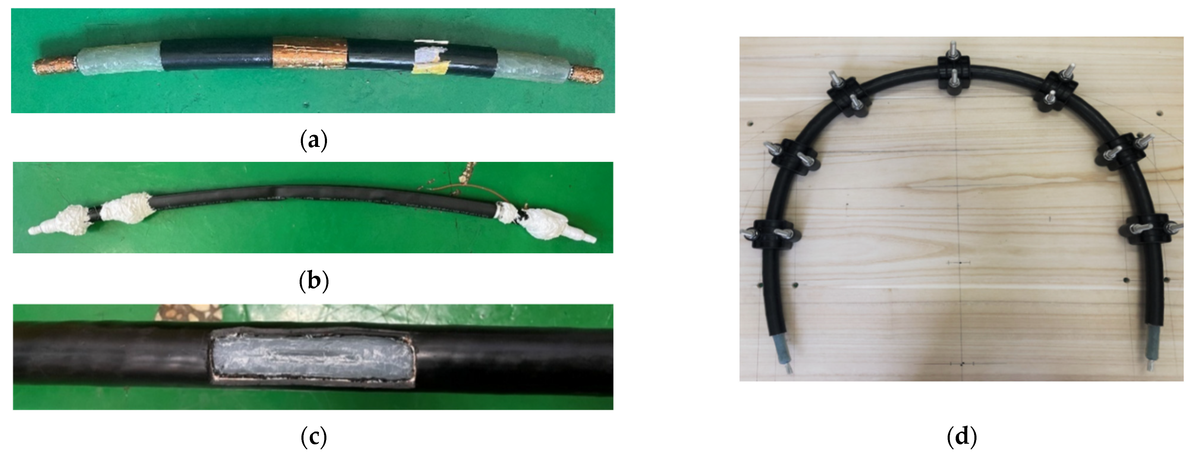
2.1. Test Specimen

The experiment selects a YJLV 8.7/15 kV-1×70 mm² distribution cable as the specimen. Except for the cable specimens of normal state, the specimens with four typical defect types, thermal aging, water ingress and dampness, insulation scratch, and excessive bending, were prepared. The cable specimens with typical defects are shown in Figure 1.

(1) Thermal Aging (Type I): A constant temperature aging chamber was employed to reproduce the thermal aging process. Due to the limitation of the chamber size, the specimen was 400 mm in length. The outer sheath, along with the copper shielding, was peeled off to evenly heat the cable insulation. Conductive silver paint was applied evenly over a length of 50 mm in the middle of the specimen, around which the copper foil was wrapped as the test electrode. According to IEC 60811, the aging temperature was set to 90 °C, and the testing time was taken in equal proportion series, that is, 12 days (mild), 24 days (moderate), and 48 days (severe). The specimen is shown in Figure 1a.

(2) Water Ingress and Dampness (Type II): Long-term operation in underground humid environments often results in cable faults caused by water ingress. The cable specimen was 1 m in length. The outer sheath with a length of 700 mm was peeled off in the middle position to expose the copper shielding. Then, 150 mm of the outer sheath was stripped from one end of the specimen, where the grounding wire was led out as the test electrode. A 700 mm long heat shrink tube was wrapped over the cable specimen. The tube was filled with tap water, and both ends were shrunk and coated with glass glue, as shown in Figure 1b. To simulate different dampness levels (mild, moderate, and severe), the grounding current was tested after 5, 10, and 15 days, respectively.

(3) Insulation Scratch (Type III): Insulation scratches often occur during the production of cable joints due to excessive cutting. The cable specimen was 1 m long. The outer sheath, copper shielding, and insulation shielding layer of the middle section were peeled off in sequence. A piece of insulation was finally peeled off to simulate the insulation scratch, as shown in Figure 1c. To simulate different scratch levels, three scratch sizes were set, that is, 40 mm × 2 mm × 1 mm (mild), 40 mm × 4 mm × 1 mm (moderate), and 40 mm × 6 mm × 2 mm (severe).

(4) Excessive Bending (Type IV): Power cables may experience irreversible distortion and damage due to prolonged or frequent bending during storage and transportation. Excessive bending damage was simulated by bending and fixing the specimen. The outer diameter (D) of the cable specimen was 30 mm. According to GB 50168-2018 [27], the minimum allowable bending radius (R_min) during installation is 600 mm (20D). To simulate different bending degrees (mild, moderate, and severe), the bending radius was separately set to 600 mm, 400 mm, and 200 mm, corresponding to specimen lengths of 2 m, 1.6 m, and 1.2 m. Cable specimens were fixed on a wooden board by cable clamps and socket head screws, as shown in Figure 1d.

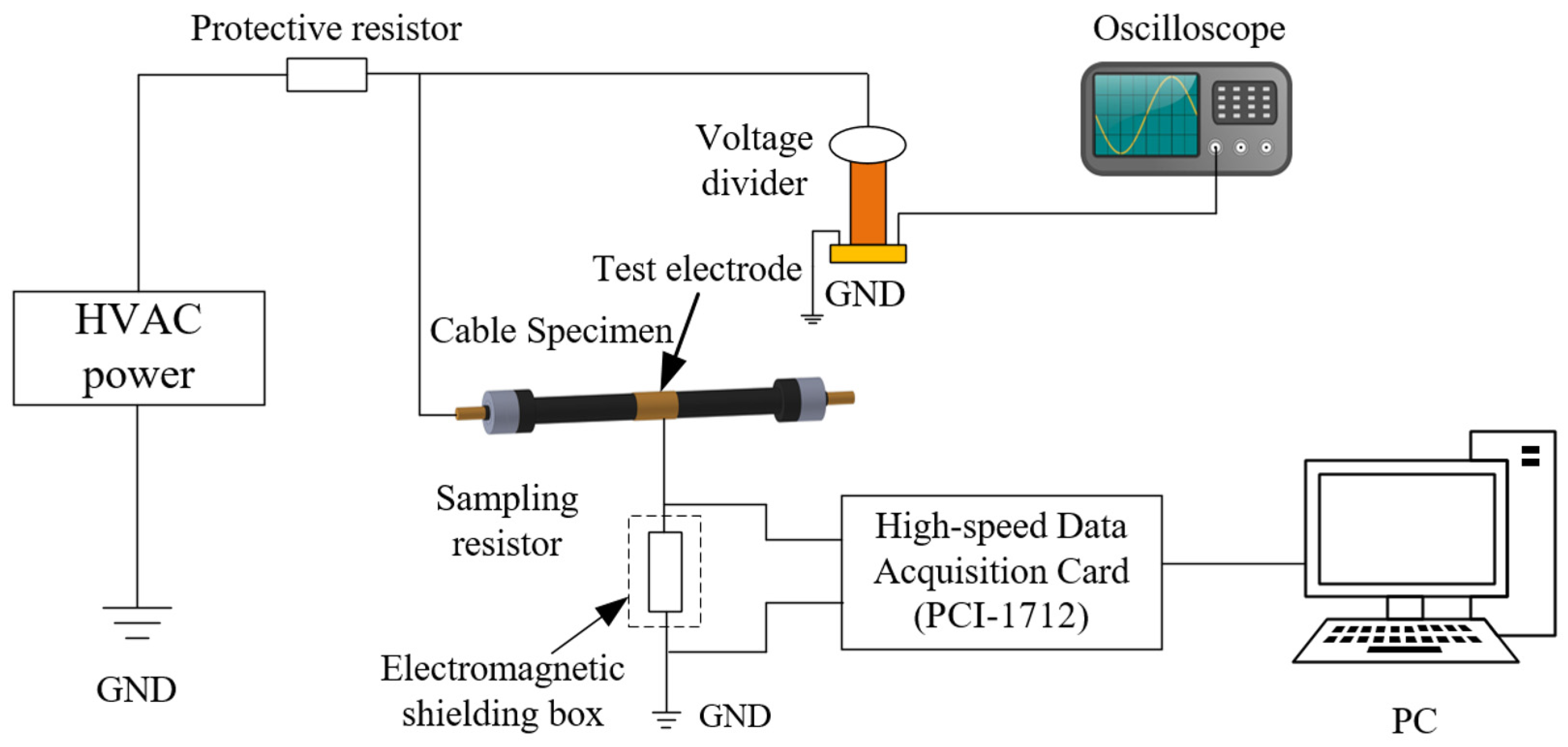
2.2. Experimental Setup

Figure 2 shows the experimental setup. The power system, consisting of a voltage regulator (TDGC2-3, CHNT, Wenzhou, China) and a testing transformer (TDM 11,000 kVA), can generate AC high voltage ranging from 0 to 50 kV. A voltage divider (RCF-50 kV) is connected to the secondary side of the transformer through the protective resistor. A portion of the voltage measured by tapping is displayed on the oscilloscope (MSO5104, RIGOL, Suzhou, China). The use of a voltage divider protects the oscilloscope from the influence of overvoltage [28]. The voltage applied to the cable specimen can be calculated according to the voltage division factor. The high-voltage terminal also connects to the specimen copper core through the protective resistor, and the copper foil testing electrode is grounded through a sampling resistor. The protective resistor has a resistance of 1 MΩ, which prevents the impact of overcurrent resulting from a short circuit. The sampling resistor, which is adjustable and non-inductive, has a resistance of 10 kΩ. The sampling resistor converts the current signal to a voltage signal. The voltage values at both ends are collected via a high-speed data acquisition card (PCI-1712) and stored in a PC with a sampling frequency of 20 kHz. The grounding current signal can eventually be obtained in the computer. According to the actual operation of the cable specimen, 8.7 kV is selected as the applied voltage. In each test, the supply voltage applied to the cable specimen is controlled consistently to the greatest extent, and it is ensured that the supply voltage presents an almost ideal sinusoidal waveform without any obvious harmonics. A total of 480 groups of grounding current data were collected, including 120 groups for each defect type (40 groups for each level).

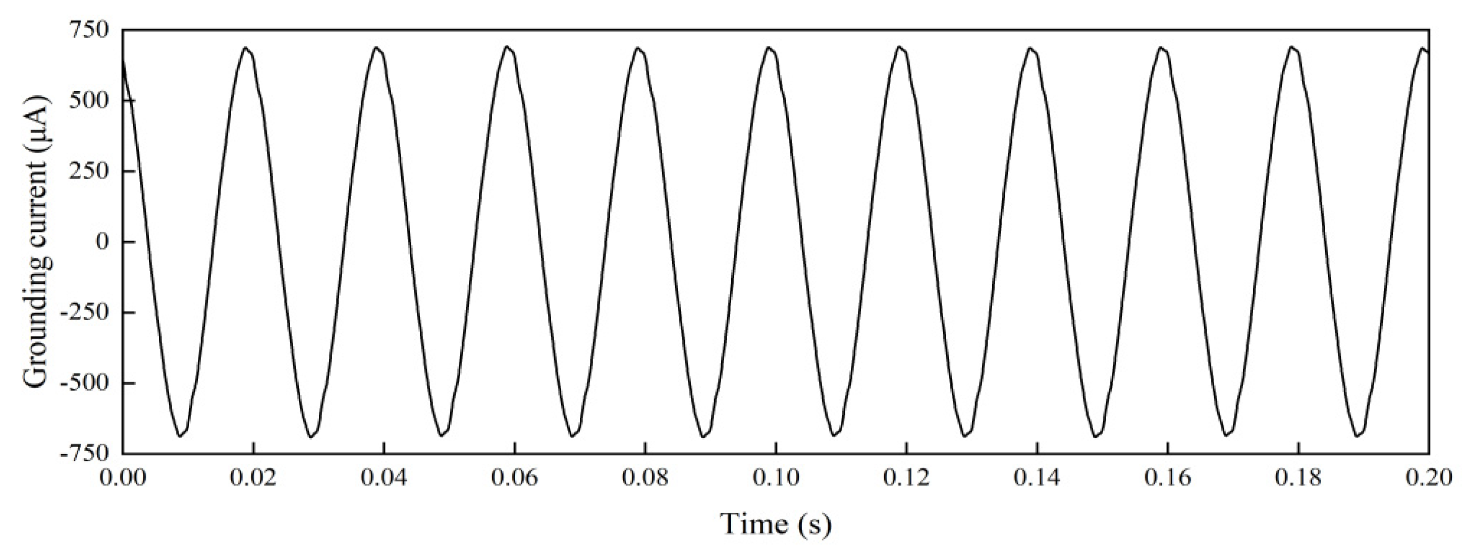
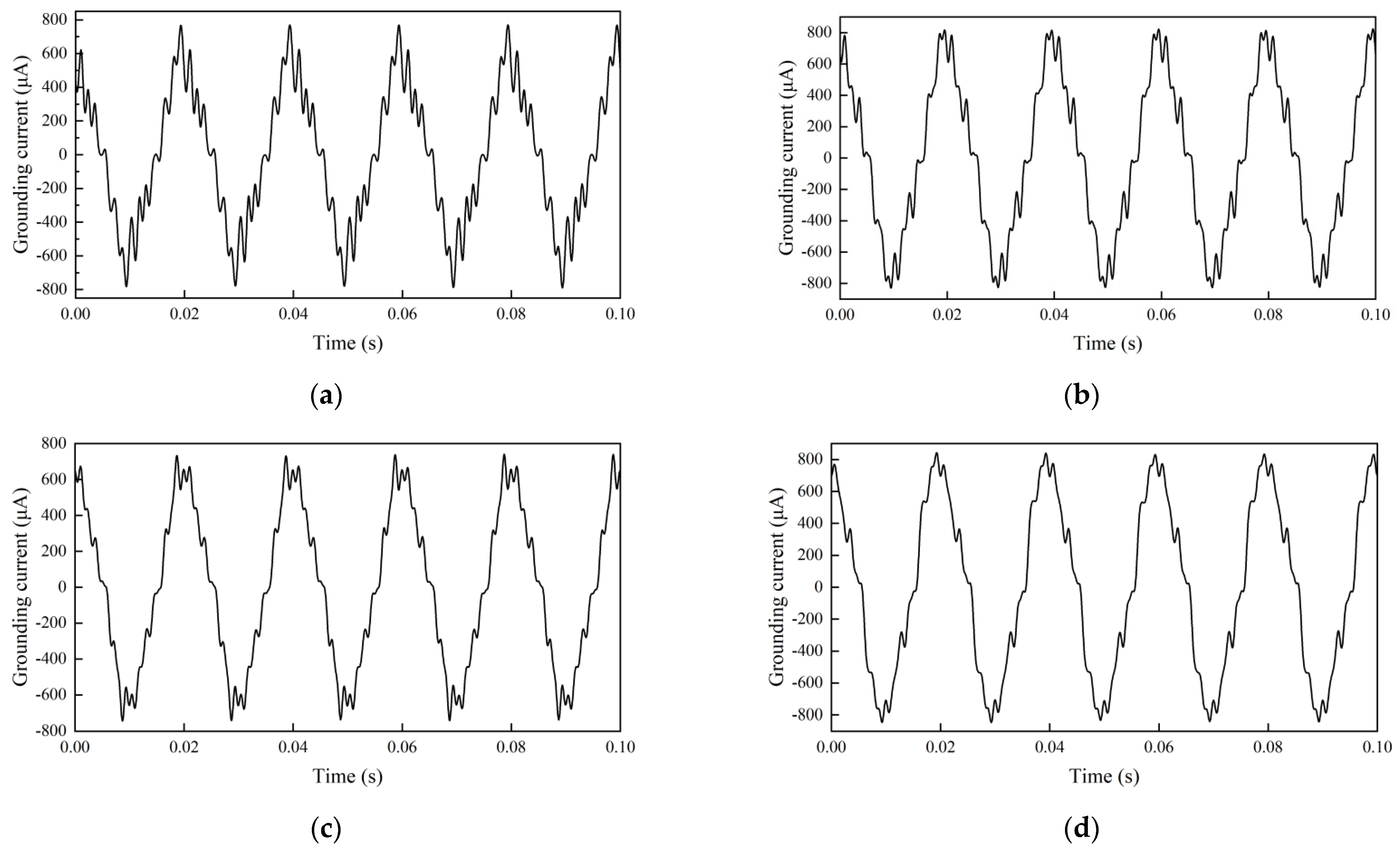
2.3. Experimental Results

As shown in Figure 3, the grounding current is approximately sinusoidal under normal conditions, with a peak value of about 690 μA. However, cable degradation causes great harmonic distortion to appear in the grounding current. The test results of cable specimens with four typical defects are shown in Figure 4. Apparently, there is a significant harmonic distortion in the grounding current when defects exist. The presence of cable defects leads to partial discharges within the cable insulation. As the partial discharge develops, the insulation gradually degrades. Changes in the performance parameters of the cable and the generation of harmonics in the voltage and current signals are the macroscopic manifestations of cable degradation. In addition, the distortion form differs depending on the defect types, which means the harmonic content of each order varies greatly.

These differences indicate that the harmonic distortion in the grounding current contains important information reflecting the cable condition. In order to present these differences in a concrete way, we attempt to transform the distortion in the linear signal into a more intuitive, stretched, and plump 2D picture. On this basis, the defect identification of problem cables can be achieved.

3. Harmonics Visualization Based on Chaotic System

3.1. Chaotic Synchronization System

The chaotic system was first proposed by American mathematician Edward Norton Lorenz in the 1960s. It is widely used in fields such as mathematics, physics, biology, meteorology, and geography. The chaotic system is a nonlinear dynamic system with uncertainty and complexity. The signal generated by chaos exhibits seemingly random, aperiodic, and disorderly motion due to the presence of the strange attractor (chaotic butterfly). The purpose of studying chaotic systems is to reveal the inherent laws and deterministic mechanisms behind such phenomena [29,30].

The chaotic synchronization system consists of a master system and a slave system. A backend controller is installed on the slave system to track the main system. The two systems are bidirectional coupled and mutually adjustable. When their signals are different, dynamic deviations form between trajectories [31]. In this study, the grounding current of the normal state cable is taken as the master system, while those of cables with defects are taken as the slave system. The dynamic deviations generated during the tracking process can reflect the harmonic differences between different cable defects.

The master and slave systems can be expressed as two nonlinear functions:

$$Master System \left\{\begin{array}{l}{\dot{u}}_1=G_1(u_1,u_2,u_3,\dots ,u_n)\\ {\dot{u}}_2=G_2(u_1,u_2,u_3,\dots ,u_n)\\ \hspace{1em}\hspace{1em}\hspace{1em} ⋮\\ {\dot{u}}_n=G_n(u_1,u_2,u_3,\dots ,u_n)\end{array}\right.$$

(1)

$$Slave System \left\{\begin{array}{l}{\dot{v}}_1=G_1(v_1,v_2,v_3,\dots ,v_n)\\ {\dot{v}}_2=G_2(v_1,v_2,v_3,\dots ,v_n)\\ \hspace{1em}\hspace{1em}\hspace{1em} ⋮\\ {\dot{v}}_n=G_n(v_1,v_2,v_3,\dots ,v_n)\end{array}\right.$$

(2)

The sequence deviation and the dynamic deviation equation between the two systems can be obtained as (3) and (4).

$$\left\{\begin{array}{l}{e}_1=u_1-v_1\\ e_2=u_2-v_2\\ \hspace{1em} ⋮\\ e_n=u_n-v_n\end{array}\right.$$

(3)

$$\left\{\begin{array}{l}{\dot{e}}_1=G_1(u_1,u_2,u_3,\dots ,u_n)-G_1(v_1,v_2,v_3,\dots ,v_n)\\ {\dot{e}}_2=G_2(u_1,u_2,u_3,\dots ,u_n)-G_2(v_1,v_2,v_3,\dots ,v_n)\\ \hspace{1em}\hspace{1em}\hspace{1em}\hspace{1em}\hspace{1em}\hspace{1em} ⋮\\ {\dot{e}}_n=G_n(u_1,u_2,u_3,\dots ,u_n)-G_n(v_1,v_2,v_3,\dots ,v_n)\end{array}\right.$$

(4)

n represents the number of equations in chaotic systems, which can be determined based on the system characteristics [32]. The trajectory deviates when a strange attractor exists. To ensure the existence of the strange attractor, we select the Lorenz chaotic synchronization system proposed by American mathematician Edward Lorenz [33]. The number of equations n of the Lorenz system is three, involving three system parameters α, β, and γ. The master and slave systems of the chaotic system can be expressed as (5) and (6).

$$Master System \left\{\begin{array}{l}{\dot{u}}_1=\alpha (u_2-u_1)\\ {\dot{u}}_2=\beta u_1-u_1{u}_3-u_2\\ {\dot{u}}_3=u_1{u}_2-\gamma u_3\end{array}\right.$$

(5)

$$Slave System \left\{\begin{array}{l}{\dot{v}}_1=\alpha (v_2-v_1)\\ {\dot{v}}_2=\beta v_1-v_1{v}_3-v_2\\ {\dot{v}}_3=v_1{v}_2-\gamma v_3\end{array}\right.$$

(6)

Assuming that the signal sequence of the main system is x, the signal sequence of the slave system is y, and the sequence data amount is m, parameters can be defined as $u_1=(x[1],x[2],\dots ,x[m-2])$, $u_2=(x[2],x[3],\dots ,x[m-1])$, $u_3=(x[3],x[4],\dots ,x[m])$, $v_1=(y[1],y[2],\dots ,y[m-2])$, $v_2=(y[2],y[3],\dots ,y[m-1])$, $v_3=(y[3],y[4],\dots ,y[m])$. The dynamic deviation equation can be calculated from (4)–(6) as a matrix.

$$\left[\begin{array}{l}{\dot{e}}_1\\ {\dot{e}}_2\\ {\dot{e}}_3\end{array}\right]=\left[\begin{array}{ccc}-\alpha & \alpha & 0\\ \beta & -1& 0\\ 0& 0& -\gamma \end{array}\right]\left[\begin{array}{l}{e}_1\\ e_2\\ e_3\end{array}\right]+\left[\begin{array}{c}0\\ -u_1{u}_3+v_1{v}_3\\ u_1{u}_2-v_1{v}_2\end{array}\right]$$

(7)

To ensure the existence of the strange attractor, the system parameters are set based on the experience of Edward Lorentz as α = 10, β = 28, and γ = 3/8. The dynamic deviation scatter diagram is drawn with ${\dot{e}}_1$ as the abscissa and ${\dot{e}}_2$ as the ordinate. In this way, the differences between the master and slave system signals are presented more intuitively and prominently.

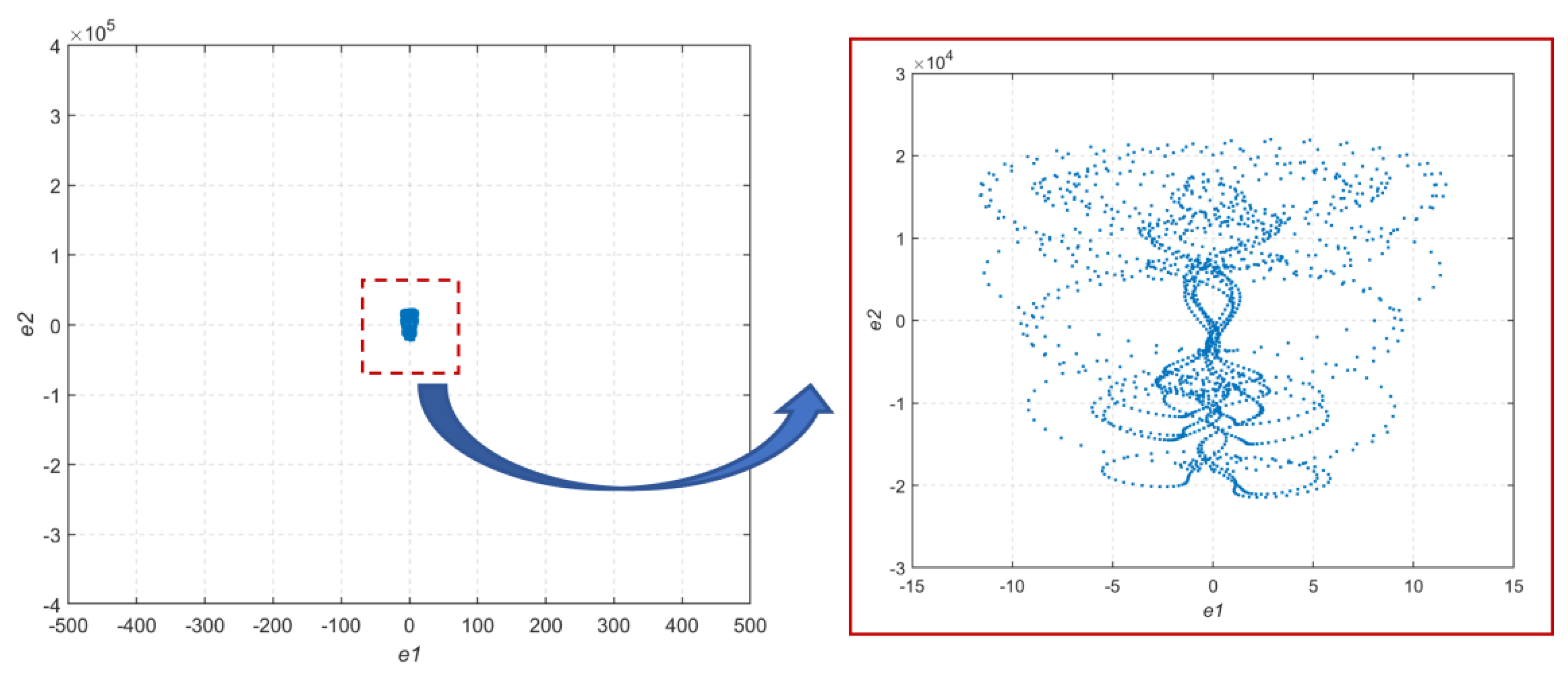
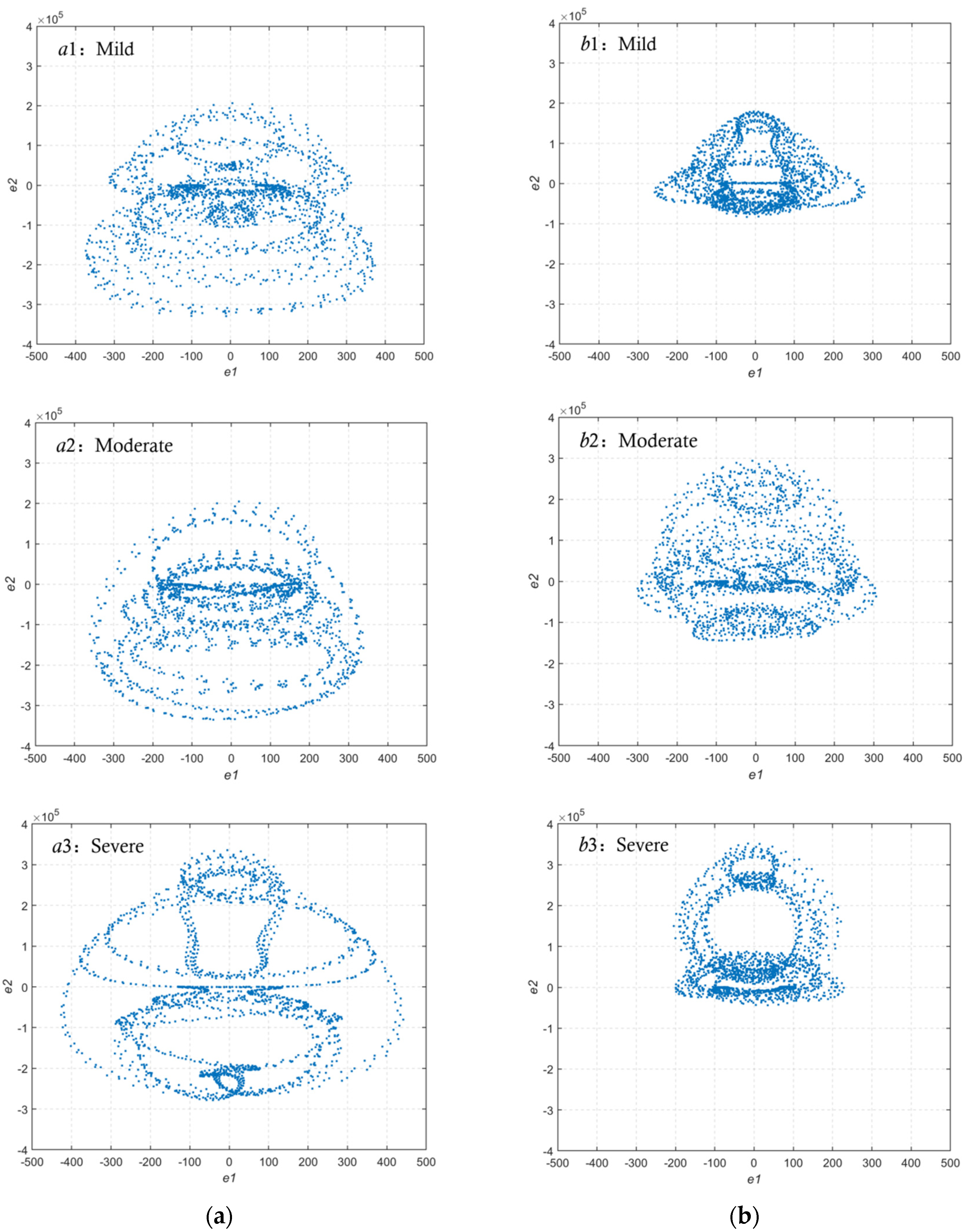
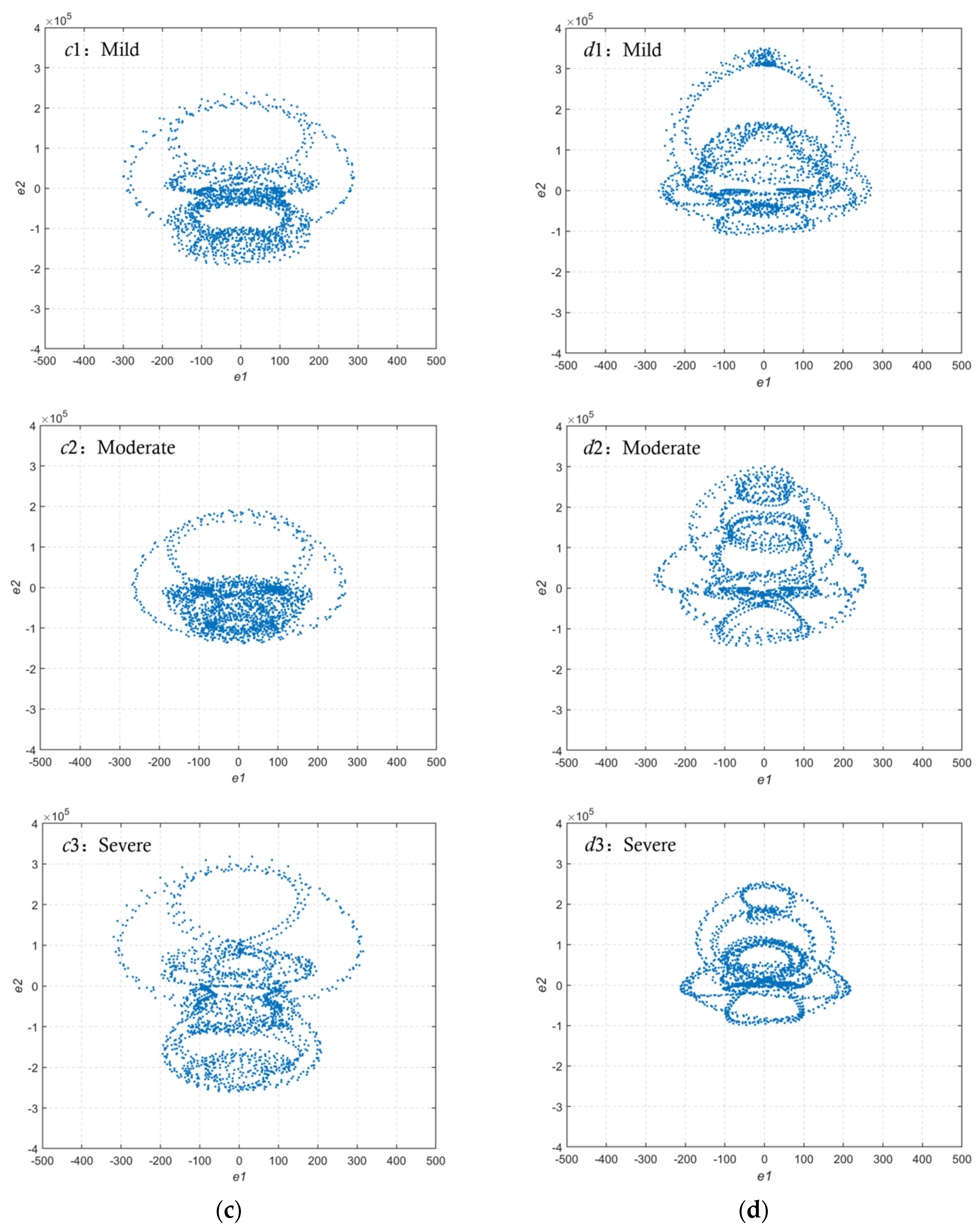
3.2. Dynamic Harmonics Scatter Diagram

This study imports the grounding current signals of the normal state and the defective cable into the master and slave systems. Five cycles of the same phase are intercepted from the signals as the input. The dynamic deviation scatter diagram obtained through the chaotic synchronization system is the 2D spatialization of the harmonic components, which are named the dynamic harmonics scatter diagrams. When the cable is in the normal state, the input signals of the master and slave systems are highly consistent. Since the dynamic deviation of the trajectory originates from the difference between the input signals of the master and slave systems, in this case, all the scatter points will be tightly concentrated around the origin in the center of the diagram. At the same coordinate scale as the defective cables, the scatter points approximately form a small patch, as shown in Figure 5. The diagram results of the cable specimens with typical defects are shown in Figure 6. The scattering range of the harmonics scatter diagram for the normal cable is much smaller than that for the defective cables by at least an order of magnitude in both the horizontal and vertical directions.

It can be observed that the dynamic harmonics scatter diagram basically presents a bilateral, symmetrical shape. The diagrams of the same cable defect have common features, but the distribution pattern of specimens with different defects varies greatly. It preliminarily indicates that the dynamic harmonics scatter diagrams can serve as the evaluation basis of cable defect identification.

As shown in Figure 6a, the scatters of thermal aging specimens are more widely distributed compared with other cable conditions. The interval length covered by e₁ ranges from 700 to 900, while that covered by e₂ ranges from 5 × 10⁵ to 6.5 × 10⁵. The overall shape of the diagram is approximately a flat ellipse. As the thermal aging deepens, the lines formed by scatter point aggregation become clearer.

As shown in Figure 6b, the scatter diagram of the water ingress specimen shows a rounded top and a wide bottom. As the dampness deepens, the distribution of scatter points undergoes a process from dense to dispersed to dense. When the dampness is mild or severe, the scatter point distribution appears as dense around and sparse in the middle.

As shown in Figure 6c, for the insulation scratch specimens, the scatter points in the upper part are sparsely distributed, while those in the lower part are densely distributed. There are two elliptical lines formed by scatter point aggregation, one large and one small, with the top tangent. The interval length covered by e₁ remains stable at around 600. As the scratch worsens, the longitudinal distribution of scatter points first gathers and then disperses.

As shown in Figure 6d, the bending degree has little effect on the overall shape of the scatter diagrams. The dynamic harmonics scatter diagram of the excessive bending specimen always exhibits a round top, a wide middle, and a narrow bottom. The interval length covered by e₁ ranges from 450 to 550, while that covered by e₂ ranges from 3.5 × 10⁵ to 4.5 × 10⁵. As the bending degree increases, the distribution area of scatter points shows a decreasing trend.

The least degraded cable of the water ingress defect seems to have the smallest dispersion, while for the cable of the excessive bending defect, the dispersion drops as the degradation deepens. There seem to be significant differences in the dispersion trends of different defects with the deepening of degradation. We tentatively believe this is related to the differences in inherent mechanisms and changes in performance parameters during the degradation process of different cable defects. Although a clear relationship between the degradation degree of each defect and the characteristics of the harmonics scatter diagrams has not yet been established, common characteristics of the same defect type, as well as significant differences between different defect types, have been identified. This can be used as a valid basis for the determination of cable defects.

Harmonics visualization was performed on the 480 groups of collected data through the chaotic synchronization system. These 480 dynamic harmonics scatter diagrams obtained will further serve as the model basis for cable condition evaluation and defect identification.

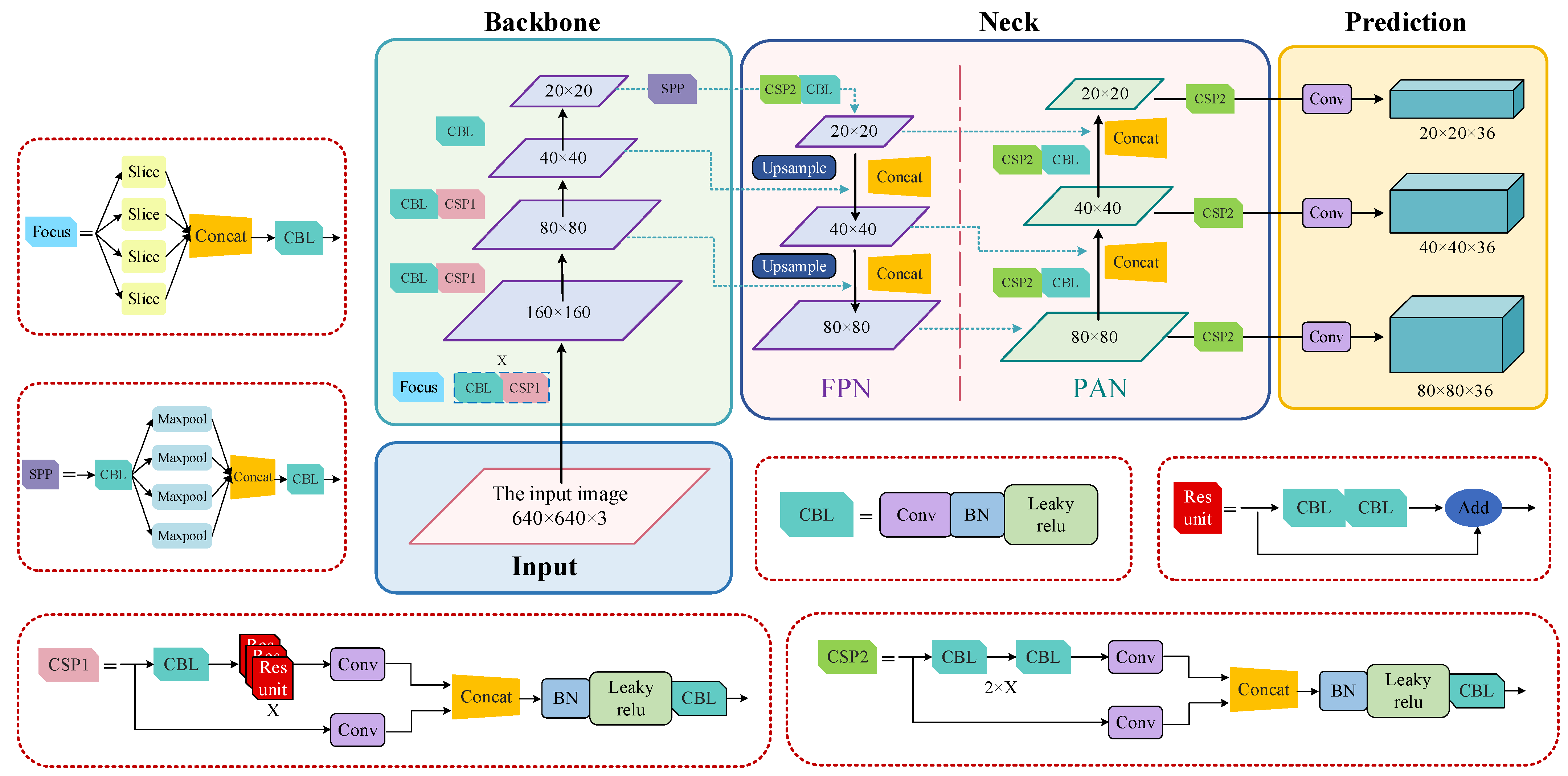
4. Defect Identification Model Based on YOLOv5

4.1. YOLOv5 Detection Algorithm

YOLO (you only look once) is a real-time target detection algorithm proposed by Joseph Redmon et al. in 2015. This is a one-stage detection method based on convolutional neural networks. Unlike traditional two-stage methods, such as R-CNN (regions with CNN features) and Fast R-CNN, YOLO adopts a single forward propagation approach, which completes the detection in a shorter time and achieves real-time performance [34,35]. Therefore, combining the YOLO algorithm with the chaotic system can achieve real-time monitoring and defect detection of dynamic harmonics scatter diagrams of cable grounding currents.

With continuous algorithm upgrading, the problems of category imbalance and data augmentation in the YOLO algorithm have been effectively solved. YOLOv5 is the latest version of the YOLO detection algorithm, which includes four models: YOLOv5s, YOLOv5m, YOLOv5l, and YOLOv5x [36]. The simplified network structure of YOLOv5 is shown in Figure 7, consisting of four parts: Input, Backbone, Neck, and Prediction.

(1) Input: Mosaic data augmentation, adaptive anchor box calculation, and adaptive image scaling are completed in this section. Mosaic data augmentation increases the diversity of training data by randomly stitching four different images, especially for images with foreground and background. Adaptive anchor box calculation automatically calculates suitable anchor boxes based on the task and dataset. The prediction bounding boxes and the iteration of network parameters depend on the initial anchor box. The input images of different sizes are uniformly scaled to the standard size through adaptive image scaling.

(2) Backbone: The Backbone network mainly comprises modules such as Focus, CBL, CSP1, SPP, etc. [37]. The internal logic of each module is clearly displayed in red dashed boxes in Figure 7. The CBL module consists of a convolutional layer (Conv), batch normalization (BN), and a Leaky ReLU activation function and is named with the first letters of each part. CSP means cross stage partial, which promotes information flow and enhances feature propagation through cross-stage connections. The SPP module, short for spatial pyramid pooling, uses maximum pooling for multi-scale feature fusion. Additionally, Concat is a concatenation operation through which tensor concatenation can be realized between different layers. Firstly, the Focus module slices the input image and generates new feature maps. This process preserves fine features while reducing computational complexity. Each CBL module contains a convolutional kernel with a size of 3 × 3 and a stride of 2 for down-sampling. The CSP module consists of two parallel branches, with the backbone branch performing initial feature extraction and the cross-stage branch connecting features of different stages to capture contextual information. The combination of CBL and CSP enables comprehensive feature extraction. The SPP module adopts a maximum pooling approach and concatenates feature maps of different scales.

(3) Neck: Referring to the PANet (pyramid attention network) architecture, this section adopts a structure of FPN+PAN. The FPN (feature pyramid network) structure transmits high-level feature information through up-sampling, while the PAN (pathway activation network) structure conveys strong localization features in the opposite direction. This pyramid structure achieves feature fusion at different levels. In addition, the convolution process in the Neck network combines CSP2 and CBL modules to enhance the ability of feature fusion.

(4) Prediction: For the feature maps of three different sizes obtained after feature fusion, processes such as the bounding box loss function (CIOU_loss) and non-maximum suppression are employed to ultimately complete the target recognition.

According to the complexity of the dynamic harmonics scatter diagrams, this study uses the YOLOv5m model to identify the cable defect type. Four anchor boxes are automatically defined. In the Backbone network, after multiple convolution operations, feature maps of three sizes, 20 × 20, 40 × 40, and 80 × 80, are extracted. Through the FPN+PAN structure, the Neck section performs two fusions of deep and shallow information through up-sampling and Concat operations. Finally, feature maps of three different sizes maximizing feature representation are output. As shown in Figure 8, the testing process can be summarized into five basic steps [36]:

(1)

Through adaptive image scaling, the dynamic scatter diagrams to be tested are unified into a fixed size of 640 × 640 and input into the YOLOv5 target recognition model.

(2)

Divide the input diagram into multiple fixed-size grids and predict multiple bounding boxes. Record the position and size information of each box and calculate the category probability.

(3)

It should be noted that the threshold judgment here is a filtering process rather than an optimization problem. Determine whether each predicted box meets the threshold according to their confidence scores and filter out the low-score boxes that do not meet the requirement. Through this process, the predicted bounding boxes that meet the specified threshold are retained, while those low-scoring boxes are eliminated.

(4)

For the retained boxes, non-maximum suppression (NMS) is used to remove high-overlap bounding boxes and retain the target box with the highest confidence.

(5)

Output the category probability along with the target box confidence and obtain the test result.

4.2. Testing Result and Comparison

The YOLOv5 target recognition model in this study is based on the harmonic visualization diagrams of grounding currents. In general cases, the problem of classification and identification of the cable state has to take the type of normal state into account. However, the method proposed in this paper has some particularities. On the one hand, from a process perspective, the comparison between the defective state and the normal state was completed in the synchronous tracking process of the chaotic system. It can be said that the dynamic harmonics scatter diagram obtained is the embodiment of the difference between the defective state and the normal state. This process is largely equivalent to completing the distinction between the normal cable and the degraded cable at this stage. On the other hand, from a results perspective, the dynamic harmonics scatter diagrams of the good cable and the degraded cable have a huge and essential difference. At the same coordinate scale, in the harmonics scatter diagram of a normal cable, almost all the scatter points are tightly concentrated around the origin to form a patch, whereas, in those of cables with different defects, the scatter points form a dispersed and differentiated pattern through aggregation. When the cable is in a normal state, there is no need for defect identification. When the cable is defective, there is also no possibility of misidentifying it as a good cable. Therefore, only the four cable defect types, thermal aging, water ingress and dampness, insulation scratch, and excessive bending, are included in this recognition model.

Table 1. Test environment.

Category	Version
Operating system	Windows 11 (64-bit)
CPU	Intel Core i7-12700H
GPU	NVIDIA GeForce RTX 3070
RAM	32 GB
Software	Python 3.10

shows the testing environment. The training set contains 300 samples of dynamic harmonics scatter diagrams, including 75 samples for each defect type (25 samples for each level). There are 180 samples of dynamics harmonics scatter diagrams in the test set, with 45 for each defect type (15 for each level). As shown in

Table 2. Identification results of cable defects.

Defect Type	Test Quantity	Accurate Quantity	Identification Accuracy/%
Thermal aging	45	44	96.67%
Water ingress and dampness	45	41
Insulation scratch	45	44
Excessive bending	45	45

, the identification accuracy is 96.67%, which verifies the effectiveness of the defect identification method based on harmonic visualization through the chaotic system. Among the four defect types, the identification accuracy of water ingress and dampness is obviously lower. The reason is that the diagrams of the medium level differ significantly from the other two, and the features are not evident. Further improvement is still needed.

The cable defect identification performance of harmonics visualization plus YOLOv5 and traditional multi-feature extraction plus back propagation neural network (BPNN) is compared under the same data source. As shown in

Table 3. Comparison with traditional feature extraction method.

Method	Harmonics Visualization + YOLOv5		Multi-Feature Extraction + BPNN
Model Establishment Procedure	Chaotic Synchronization System	YOLOv5	Harmonics Separation	Multi-Feature Extraction	mRMR Feature Selection	PCA Feature Fusion	BPNN
Test Time/s	1.23	0.33	0.42	0.51	/	0.75	0.86
Identification Accuracy/%	96.67%		95.56%

, the method proposed in this paper only requires one harmonics visualization operation through the chaotic synchronization system before YOLOv5. The image feature extraction relies on convolution operations in Backbone, and the fusion of deep and shallow features is completed in Neck. However, the entire process of the traditional feature extraction method includes five major steps: harmonics separation, multi-feature extraction (minimum-redundancy-maximum-relevance, mRMR), feature selection (principal component analysis, PCA), feature fusion, and BPNN. The pre-processing work before model training and testing is cumbersome and professional. The overall testing time of the proposed method is also superior to that of the traditional feature extraction method. The identification accuracy of harmonics visualization plus YOLOv5 is 96.67%, which is slightly higher than 95.56% for multi-feature extraction plus BPNN. In conclusion, the harmonics visualization plus YOLOv5 method has improved in terms of workload, detection time, and identification accuracy.

5. Conclusions

This study conducted a grounding current test, took grounding current signals of cable specimens with four typical defects as the information source, transformed the harmonic distortion into 2D visualized images through the chaotic synchronization system, and established an intelligent target recognition model based on the YOLOv5 algorithm to identify cable defects. The main conclusions are as follows.

(1)

Cable defects reduce the insulation performance, induce the appearance of harmonic distortion within grounding currents, and increase signal amplitude to various degrees.

(2)

The dynamic harmonics scatter diagram (visualized harmonics) basically presents a bilateral symmetrical shape. The diagrams of the same cable defect have common features, but the distribution pattern of different defects varies greatly. Representative features include overall shape, distribution range, density degree, and typical lines formed by scatter aggregation.

(3)

Among the four defect types, the harmonics scatter diagram of thermal aging has the widest scatter distribution, presenting an overall elliptical shape. The representative feature of insulation scratch is that two elliptical lines formed by clustered scatter points, one large and one small, touch at the top. Excessive bending exhibits the most consistent scatter shape across different degradation degrees, with a round top, wide middle, and narrow bottom. The image features of water ingress and dampness are less obvious compared with the other three defect types.

(4)

A YOLOv5 target recognition model based on the dynamic harmonics scatter diagrams is proposed, through which the identification of four typical cable defects, thermal aging, water ingress and dampness, insulation scratch, and excessive bending, is achieved. This approach is verified to be more accurate, less time-consuming, and requires less workload compared with the traditional feature extraction method.

(5)

The proposed method effectively retains the information contained in the grounding current distortion of defective cables. The use of the chaotic synchronization system reduces the difficulty of data analysis and presents harmonic information in a more focused and distinguishable way. Fewer steps will reduce the complexity, professional difficulty, and required time of cable defect detection while ensuring good detection accuracy. It provides a new technical means for online monitoring of power cables and can further ensure the safe operation of cable lines.

(6)

The core of the method proposed is to transform the harmonic distortion of signals into visualized images. It is not limited to analyzing cable grounding currents but can be used as a distortion analysis tool for various signals (voltage, current, etc.). Through adaptive adjustments, this method can be potentially extended to the state assessment of other electrical equipment or even other issues in the power system.

(7)

In this study, the grounding current measurements on normal and defective cables were not performed simultaneously due to limitations in sample size and test site. We ensured the waveform quality of the supply voltage (an almost ideal sinusoidal waveform without any obvious harmonics) during each test to largely exclude the influence of main harmonics on the test results. However, in real power grids, main harmonics are always present, uncontrollable, and may be different at different times. An instantaneous grounding current test with a good cable is necessary so that the influence of the mains harmonics would be excluded during the tracking process to make the proposed techniques desirable for continuous cable monitoring.

(8)

At present, the proposed method is still in the laboratory research stage. Factors in practical applications, such as cable laying conditions and the testing environment, have not been fully considered. In addition, this method can effectively identify the types of cable defects, but a clear relationship between the degradation degree of each defect and the characteristics of harmonics scatter diagrams has not yet been established. Developing a high-precision supporting sensor based on the actual situation and optimizing the analysis technique to assess the degradation degree of power cables will be the focus of our future work.

References

1. Fetisov, S.; Zubko, V.; Steiner, C.; Nosov, A.; Zanegin, S.; Vysotky, V. Review of the design, production and tests of compact AC HTS power cables. Prog. Supercond. Cryog. 2021, 22, 31–39. [Google Scholar]
2. Winkelmann, E.; Shevchenko, I.; Steiner, C.; Kleiner, C.; Kaltenborn, U.; Birkholz, P.; Schwarz, H.; Steiner, T. Monitoring of Partial Discharges in HVDC Power Cables. IEEE Electr. Insul. Mag. 2022, 38, 7–18. [Google Scholar] [CrossRef]
3. Chang, C.K.; Lai, C.S.; Wu, R.N. Decision Tree Rules for Insulation Condition Assessment of Pre-molded Power Cable Joints with Artificial Defects. IEEE Trans. Dielectr. Electr. Insul. 2019, 26, 1636–1644. [Google Scholar] [CrossRef]
4. Chojnacki, A.L. Analysis of Seasonality and Causes of Equipment and Facility Failures in Electric Power Distribution Networks. Prz. Elektrotechniczny 2023, 99, 157–163. [Google Scholar] [CrossRef]
5. Zhu, L.; Li, Z.; Hou, K. Effect of radical scavenger on electrical tree in cross-linked polyethylene with large harmonic superimposed DC voltage. High Volt. 2023, 8, 739–748. [Google Scholar] [CrossRef]
6. Du, B.X.; Han, C.; Li, Z.; Li, J. Effect of graphene oxide particles on space charge accumulation in LDPE/GO nanocomposites. IEEE Trans. Dielectr. Electr. Insul. 2018, 25, 1479–1486. [Google Scholar] [CrossRef]
7. Li, Z.L.; Du, B.X.; Yang, Z.R.; Han, C.L. Temperature dependent trap level characteristics of graphene/LDPE nanocomposites. IEEE Trans. Dielectr. Electr. Insul. 2018, 25, 137–144. [Google Scholar] [CrossRef]
8. Marzinotto, M.; Mazzanti, G. The Feasibility of Cable Sheath Fault Detection by Monitoring Sheath-to-ground Currents at the Ends of Cross-bonding Sections. IEEE Trans. Ind. Appl. 2015, 51, 5376–5384. [Google Scholar] [CrossRef]
9. Haikali, E.N.N.; Nyamupangedengu, C. Measured and simulated time-evolution PD characteristics of typical installation defects in MV XLPE cable terminations. SAIEE Afr. Res. J. 2019, 110, 136–144. [Google Scholar] [CrossRef]
10. Li, Z.; Qian, Y.; Wang, H.; Zhou, X.L.; Sheng, G.H.; Jiang, X.C. A Novel Image-orientation Feature Extraction Method for Partial Discharges. IET Gener. Transm. Distrib. 2022, 16, 1139–1150. [Google Scholar] [CrossRef]
11. Li, L.; Yong, J. A new method for on-line cable tanδ monitoring. In Proceedings of the International Conference on Harmonics and Quality of Power (ICHQP), Ljubljana, Slovenia, 13–16 May 2018; pp. 1–6. [Google Scholar]
12. Jiang, J.; Ge, Z.D.; Zhao, M.X.; Yu, M.; Chen, X.W.; Chen, M.; Li, J.S. A Capacitive Strip Sensor for Detecting Partial Discharge in 110-kV XLPE Cable Joints. IEEE Sens. J. 2018, 18, 7122–7129. [Google Scholar] [CrossRef]
13. Borghetto, J.; Pirovano, G.; Tornelli, C.; Contin, A. Off-Line and Laboratory On-Line PD Tests on Thermally Aged MV Cable Joints. In Proceedings of the 2019 IEEE Electrical Insulation Conference (EIC), Calgary, AB, Canada, 16–19 June 2019; pp. 418–422. [Google Scholar]
14. Rosle, N.; Muhamad, N.A.; Rohani, M.N.K.H.; Jamil, M.K.M. Partial Discharges Classification Methods in XLPE Cable: A Review. IEEE Access 2021, 9, 133258–133273. [Google Scholar] [CrossRef]
15. Montanari, G.C.; Ghosh, R. An Innovative Approach to Partial Discharge Measurement and Analysis in DC Insulation Systems During Voltage Transient and in Steady State. High Volt. 2021, 6, 565–575. [Google Scholar] [CrossRef]
16. Wang, X.; Jiang, Q.X.; Wu, C.; Liu, S.; Wu, K. Study on Space Charge Characteristics in XLPE Under DC Voltage Superimposed by Impulse Voltage. IEEE Trans. Dielectr. Electr. Insul. 2023, 30, 184–192. [Google Scholar] [CrossRef]
17. Sternes, H.H.; Aakervik, J.; Hvidsten, S. Water Treeing in XLPE Insulation at a Combined DC and High Frequency AC Stress. In Proceedings of the 2013 IEEE Electrical Insulation Conference (EIC), Ottawa, ON, Canada, 2–5 June 2013; pp. 494–498. [Google Scholar]
18. Rui, Y.; Hird, R.; Yin, M.; Soga, K. Detecting Changes in Sediment Overburden Using Distributed Temperature Sensing: An Experimental and Numerical Study. Mar. Geophys. Res. 2019, 40, 261–277. [Google Scholar] [CrossRef]
19. Xu, K.; Wang, W.; Yuan, C. A Fault Location Analysis of Optical Fiber Communication Links in High Altitude Areas. Electronics 2023, 12, 3728. [Google Scholar] [CrossRef]
20. Sun, X.; Li, W.K.; Hou, Y.H.; Pong, P.W.T. Underground Power Cable Detection and Inspection Technology Based on Magnetic Field Sensing at Ground Surface Level. IEEE Trans. Magn. 2014, 50, 1–5. [Google Scholar] [CrossRef]
21. Zhu, G.; Zhou, K.; Lu, L.; Li, Y.; Xi, H.; Zeng, Q. Online Monitoring of Power Cables Tangent Delta Based on Low-Frequency Signal Injection Method. IEEE Trans. Instrum. Meas. 2021, 70, 1–8. [Google Scholar] [CrossRef]
22. Waluyo; Fauziah, D.; Khaidir, I.M. The Evaluation of Daily Comparative Leakage Currents on Porcelain and Silicone Rubber Insulators Under Natural Environmental Conditions. IEEE Access 2021, 9, 27451–27466. [Google Scholar] [CrossRef]
23. Zhou, T.; Zhu, X.Z.; Yang, H.F.; Yan, X.Y.; Jin, X.J.; Wan, Q.Z. Identification of XLPE cable insulation defects based on deep learning. Glob. Energy Interconnect.-China 2023, 6, 36–49. [Google Scholar] [CrossRef]
24. Liu, Y.; Wang, H.; Zhang, H.; Du, B.X. Thermal Aging Evaluation of XLPE Power Cable by Using Multidimensional Characteristic Analysis of Leakage Current. Polymers 2022, 14, 3147. [Google Scholar] [CrossRef] [PubMed]
25. Hu, R.; Sun, W.X.; Lu, X.; Tang, F.; Xu, Z.F.; Tian, J.; Zhang, D.N.; Li, G.C. Effect of Interface Defects on the Harmonic Currents in Distribution Cable Accessories under Damp Conditions. Coatings 2023, 13, 1430. [Google Scholar] [CrossRef]
26. Kemari, Y.; Mekhaldi, A.; Teguar, M. Experimental Investigation and Signal Processing Techniques for Degradation Assessment of XLPE and PVC/B Materials under Thermal Aging. IEEE Trans. Dielectr. Electr. Insul. 2017, 24, 2559–2569. [Google Scholar] [CrossRef]
27. GB 50168-2018; Standard for Construction and Acceptance of Cable Line Electric Equipment Installation Engineering. China Planning Press: Beijing, China, 2018.
28. Deb, S.; Das, S.; Pradhan, A.K.; Banik, A.; Chatterjee, B.; Dalai, S. Estimation of Contamination Level of Overhead Insulators Based on Surface Leakage Current Employing Detrended Fluctuation Analysis. IEEE Trans. Industr. Electro. 2020, 67, 5729–5736. [Google Scholar] [CrossRef]
29. Yau, H.T.; Wang, M.H. Chaotic Eye-based Fault Forecasting Method for Wind Power Systems. IET Renew. Power Gener. 2015, 9, 593–599. [Google Scholar] [CrossRef]
30. Wang, M.H.; Lu, S.D.; Liao, R.M. Fault Diagnosis for Power Cables Based on Convolutional Neural Network With Chaotic System and Discrete Wavelet Transform. IEEE Trans. Power Deliv. 2022, 37, 582–590. [Google Scholar] [CrossRef]
31. Chen, C.; Zhu, D.; Wang, L.; Zeng, L. One-Dimensional Quadratic Chaotic System and Splicing Model for Image Encryption. Electronics 2023, 12, 1325. [Google Scholar] [CrossRef]
32. Ding, D.; Wang, W.; Yang, C.; Kleiner, Z.; Hu, Y.; Wang, J.; Wang, M.; Niu, Y.; Zhu, H. An n-dimensional modulo chaotic system with expected Lyapunov exponents and its application in image encryption. Chaos Solitons Fractals 2023, 174, 113841. [Google Scholar] [CrossRef]
33. Zhang, J.; Zhu, X.; Yin, B.; Zeng, L. A new fifth-dimensional Lorentz hyper-chaotic system and its dynamic analysis, synchronization and circuit experiment. Mod. Phys. Lett. B 2022, 36, 2250080. [Google Scholar] [CrossRef]
34. Zhang, T.; Zhang, Y.N.; Xin, W.; Liao, J.S.; Xie, Q.F. A Light-Weight Network for Small Insulator and Defect Detection Using UAV Imaging Based on Improved YOLOv5. Sensors 2023, 23, 5249. [Google Scholar] [CrossRef]
35. Huang, Y.; Jiang, L.; Han, T.; Xu, S.; Liu, Y.; Fu, J. High-Accuracy Insulator Defect Detection for Overhead Transmission Lines Based on Improved YOLOv5. Appl. Sci. 2022, 12, 12682. [Google Scholar] [CrossRef]
36. Lu, Y.; Qiu, Z.; Liao, C.; Zhou, Z.; Li, T.; Wu, Z. A GIS Partial Discharge Defect Identification Method Based on YOLOv5. Appl. Sci. 2022, 12, 8360. [Google Scholar] [CrossRef]
37. Yuan, S.; Du, Y.; Yin, B.; Liu, M.; Yue, F.; Li, B.; Zhang, H. YOLOv5-Ytiny: A Miniature Aggregate Detection and Classification Model. Electronics 2022, 11, 1743. [Google Scholar] [CrossRef]
Figure 1. Cable specimens with typical defects: (a) thermal aging; (b) water ingress and dampness; (c) insulation scratch; (d) excessive bending.
Electronics 13 01159 g001
Figure 2. Experimental setup of AC grounding current test.
Electronics 13 01159 g002
Figure 3. The grounding current of the cable specimen of normal state.
Electronics 13 01159 g003
Figure 4. The grounding currents of cable specimens with typical defects (moderate level): (a) thermal aging; (b) water ingress and dampness; (c) insulation scratch; (d) excessive bending.
Electronics 13 01159 g004
Figure 5. The dynamic harmonics scatter diagram of the normal cable.
Electronics 13 01159 g005
Figure 6. Dynamic harmonics scatter diagrams of cable specimens with typical defects: (a) thermal aging; (b) water ingress and dampness; (c) insulation scratch; (d) excessive bending. Each includes three sub-graphs of defect level: mild, moderate, and severe.
Electronics 13 01159 g006aElectronics 13 01159 g006b
Figure 7. YOLOv5 network main structure.
Electronics 13 01159 g007
Figure 8. YOLOv5 test flowchart.
Electronics 13 01159 g008