Modeling and Analyzing the Strategy Game “Factorio” Using Modular Petri Nets and the General-Purpose Petri Net Simulator

Abstract

The video game Factorio is a popular real-time strategy game that hosts a variety of gameplay scenarios analogous to real-world problems such as factory building, pipeline optimization, and conveyor belt logistics. It also considers environmental costs such as pollution and energy consumption. This game focuses on automation and resource management within the context of creating and maintaining factories. Players are challenged to design efficient factories, automate production, control energy consumption, and balance resource utilization, all while defending against environmental challenges such as pollution and hostile enemies. Factorio is a complex software; however, studies have demonstrated its ability to enhance student satisfaction when integrated as an educational module at the university level. This paper aims to utilize the power of Petri Net theory and the practical tool GPenSIM to model and simulate several Factorio pipelines and score them against one another, exploring which pipeline configuration is optimal. The primary objective is to make a mathematical model (Petri Net) to better understand the game’s complex mechanisms, identify bottlenecks within the system, and explore opportunities for optimization within the network of modules. The insights gained from this paper may find practical applications in real-world scenarios.

1. Introduction

Factorio is a popular real-time strategy game focused on automation and resource management in creating and maintaining factories. Players are challenged to design efficient factories, automate production, control energy consumption, and balance resource utilization, all while defending against environmental challenges such as pollution and hostile enemies. Factorio’s complexity has made it a research subject, and studies have demonstrated its ability to enhance student satisfaction when integrated as an educational module at the university level [1].

This paper aims to leverage the power of discrete simulation using Petri Net theory and the tool GPenSIM to model and simulate Factorio’s gameplay. Its primary objective is to make a mathematical model (Petri Net) to better understand the game’s complex mechanisms, identify bottlenecks within the system, and explore opportunities for optimization within the network of modules. The insights gained from this paper may find practical applications in real-world scenarios.

1.1. Problem Definition

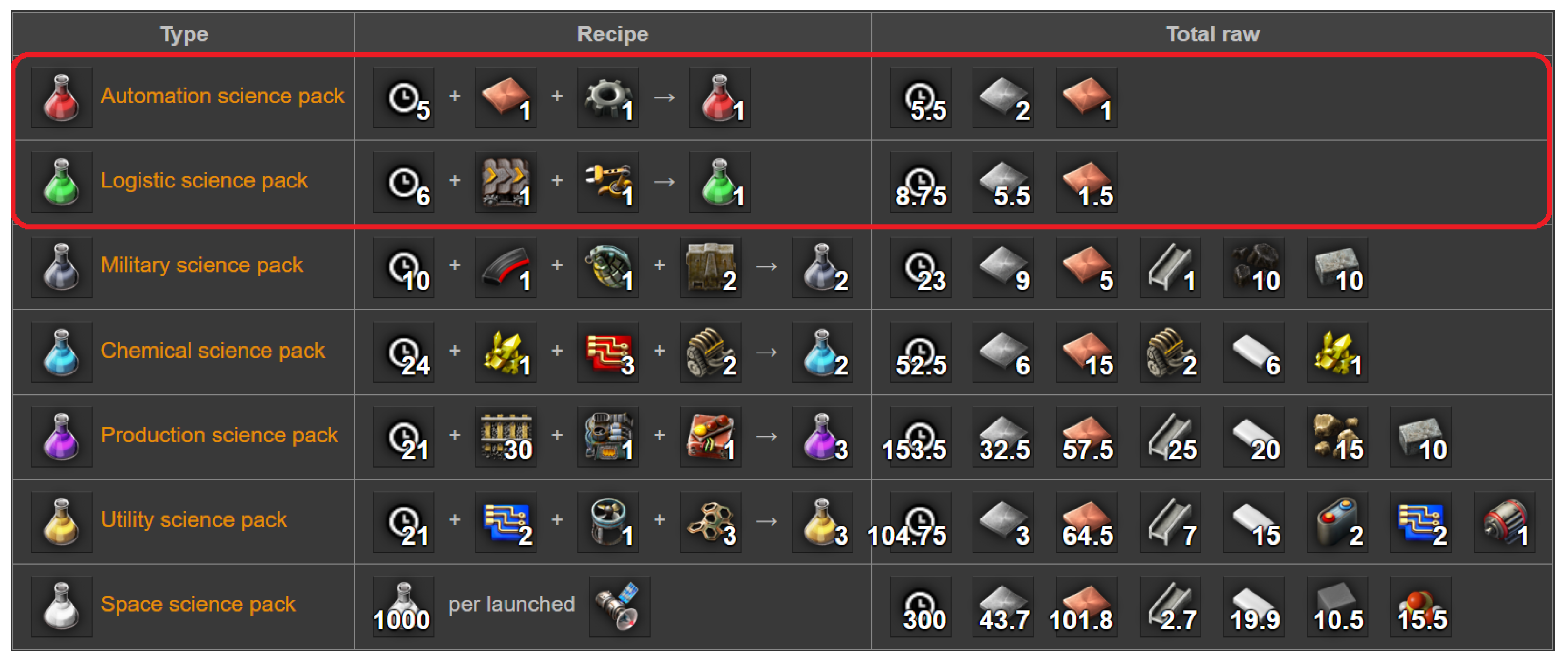
The scope of this paper includes models and simulations for a range of production pipelines designed for the manufacturing of Automation and Logistic science packs. Throughout this paper, the terms “Automation” and “Logistic science packs” are often referred to as “red” and “green” science packs, respectively, and are used interchangeably.

Science packs are essential items that enable further in-game research, unlocking new recipes for crafting advanced items. These packs are, therefore, instrumental for game progression. Factorio has seven different science packs, as shown in Figure 1, but for this paper’s scope, the selected science packs will suffice.

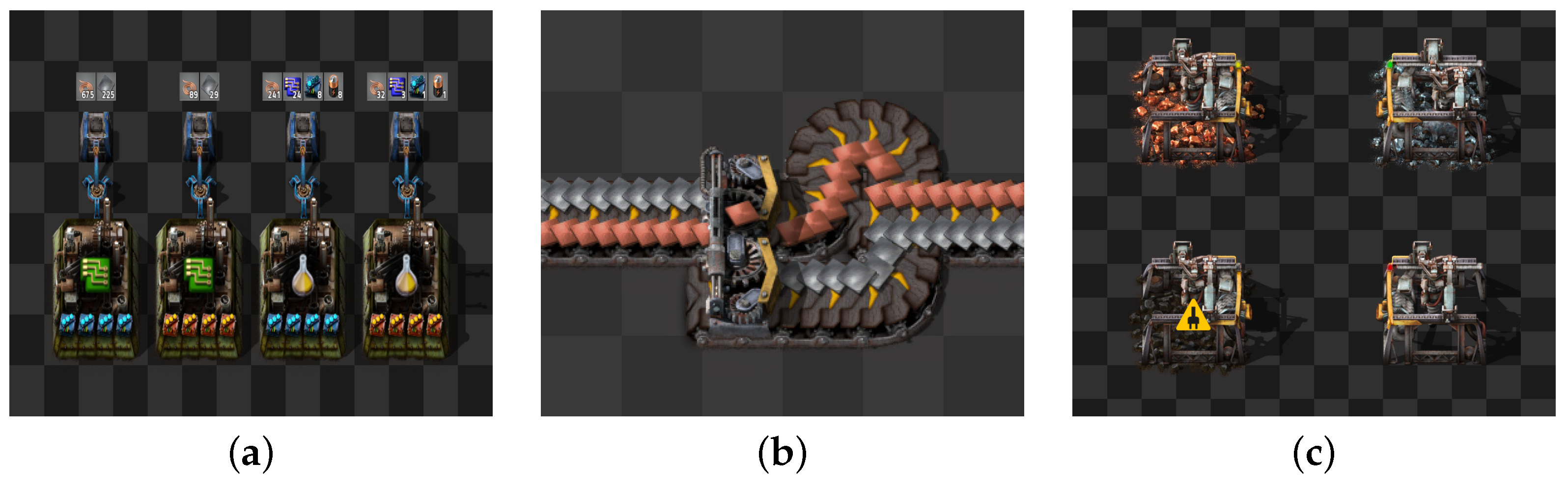
This modeling process considers various costs, including energy consumption and pollution levels, to determine the most efficient pipeline. Completing such a pipeline will entail the following (Figure 2):

• Resource Extraction: Extracting raw minerals necessary for producing red science packs.
• Assembling Machines: Allowing automated production of new items given the necessary ingredients.
• Speed Modules: Factorio speed modules enhance the crafting speed of assembling machines at the cost of greater energy consumption.
• Transportation and Logistics: Moving items from one machine to another using conveyor belts and mechanical arms (inserters).
• Pollution: Assessing the environmental consequences associated with each production pipeline, including pollution levels.
• Energy Consumption: Evaluating the energy demands of the entire process.

Figure 2. Frequently used machines in Factorio. (a) Assembling machines. (b) Conveyor belts. (c) Electric mining drills.

Figure 2. Frequently used machines in Factorio. (a) Assembling machines. (b) Conveyor belts. (c) Electric mining drills.

1.2. Relevant Works

A few research papers have studied Factorio [2,3,4], mainly dealing with optimizing conveyor belts. A bachelor thesis on “Verification of Factorio belt balancers using Petri Nets” is similar to our work as it uses Petri Nets [5]; however, this work focuses on describing Belt Balancer properties with Linear Temporal Logic (LTL [6]) and then tries automatic verification of those properties (with PROMELA [7]). Some other works (e.g., [1]) study the usefulness of Factorio as a tool for teaching students about logistics.

The structure of this paper is as follows: Section 2 formally defines Petri Nets and introduces the tool GPenSIM. Section 3 presents the design approach and the resulting modular Petri Net model. Section 4 presents the implementation of the modular Petri Net model with GPenSIM. Section 5 presents the results and an analysis of the results. Section 6 is for discussion.

2. Petri Nets and GPenSIM

This paper aims to develop a Modular Petri Net model of the production pipeline. The developed model is then implemented using the GPenSIM toolbox for simulation. This section starts with formal definitions of Petri Nets and then gives a short introduction to GPenSIM.

2.1. Petri Nets: Definition

Petri Net (P/T Petri Net) is defined as a four-tuple [8,9]:

$$PTPN=(P,T,F,M_0),$$

where,

• P: set of places, $P=\{p_1,p_2,\dots ,p_{n_p}\}.$
• T: set of transitions, $T=\{t_1,t_2,\dots ,t_{n_t}\}$.
  P∩T = ∅.
• F: set of directed arcs; $F\subseteq (P\times T)\cup (T\times P).$ The default arc weight W of $f_{ij}$ ($f_{ij}\in F$, an arc going from $p_i$ to $t_j$ or from $t_i$ to $p_j)$ is singleton, unless stated otherwise.
• M: row vector of markings (tokens) on the set of places.
  $M=[M\left(p_1\right),M\left(p_2\right),\dots ,M\left(p_{n_p}\right)]\in N^{n_p}$, $M_0$ is the initial marking.

2.2. Modular Petri Nets: Definition

A Modular Petri Net is composed of one or more Petri Modules and zero or more Inter-Modular Connectors (IMCs). The definition of Modular Petri Net is lengthy; due to brevity, it is not given here. The interested reader is referred to [10].

Modular Petri Nets allow independent development of testing of Petri Modules before they are put together in the overall model by the IMCs [10]. Also, the Petri Modules can run on different computers. Hence, Modular Petri Nets allow faster development and simulation (because of the deployment of many computers).

2.3. GPenSIM

GPenSIM (General-Purpose Petri Net Simulator) is a MATLAB toolbox developed by the second author of this paper [11] and is freely available [12]. Researchers use GPenSIM’s coloring capabilities to develop Petri Net models of real-life discrete systems [13]. Also, GPenSIM allows modeling large discrete systems with a modular approach [10].

3. Method and Design

Section 3.1 presents the overall design and the resulting Modular Petri Net model. The individual modules of the model are described in Section 3.2. The final section, Section 3.3, presents some design parameters.

3.1. Overall Design

The overall design of the science pack production pipeline follows a Main Bus design system. The Main Bus system is an organized approach that strategically centralizes the most frequently used and essential ingredients for assembling machines. This design philosophy addresses the common issue of chaotic and overly complex factory layouts often referred to as spaghetti factories. By implementing a Main Bus, we are striving to enhance the organization and maintainability of the production pipeline while ensuring a steady and well-managed flow of resources [14].

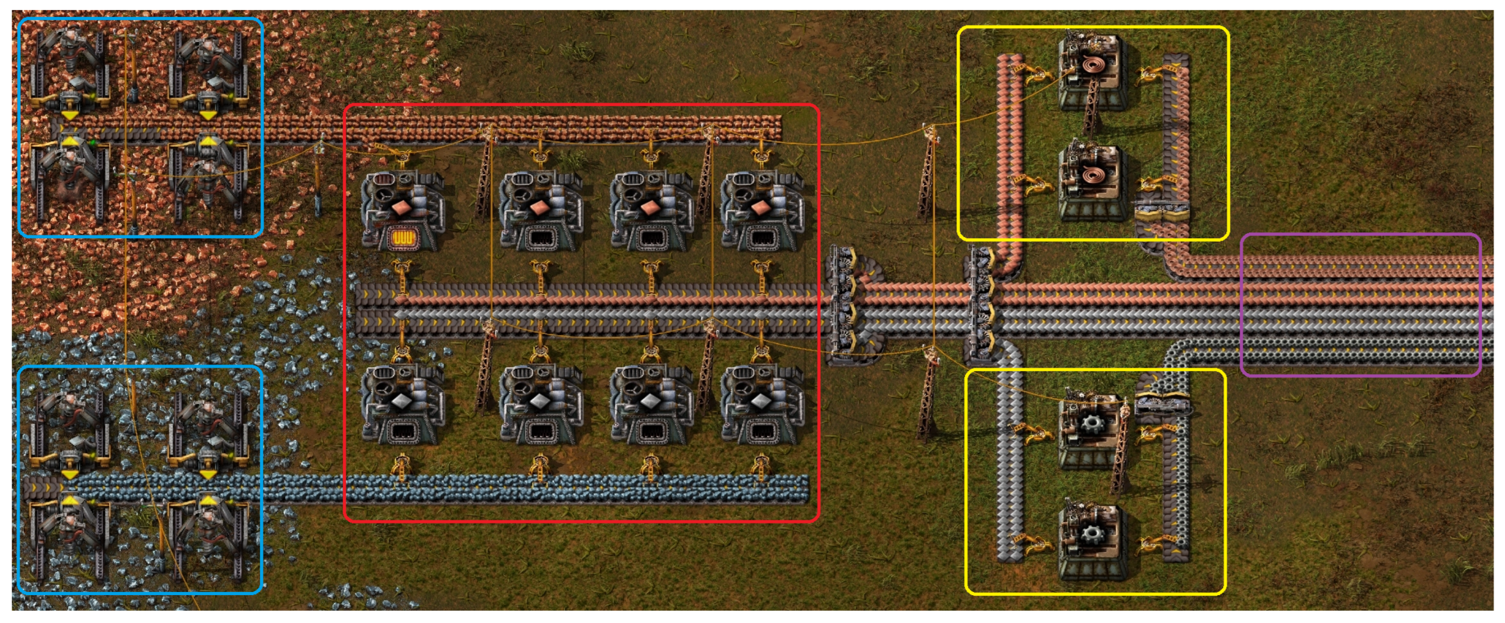
Figure 3 visually represents the initial stage of the Main Bus design system.

In this design, the process begins with the extraction of raw minerals using electric mining drills. These minerals are then transported via conveyor belts and inserted into electric furnaces using inserters (mechanical arms). Once processed, the refined minerals are placed back onto the conveyor belts, serving as the foundation of our bus and ready for use by various downstream machines.

Additionally, Figure 3 demonstrates the use of splitters, a specialized conveyor belt component, to extract specific materials from the bus. Assembling machines may craft the desired item and forward that item back onto the bus.

3.2. The Modules

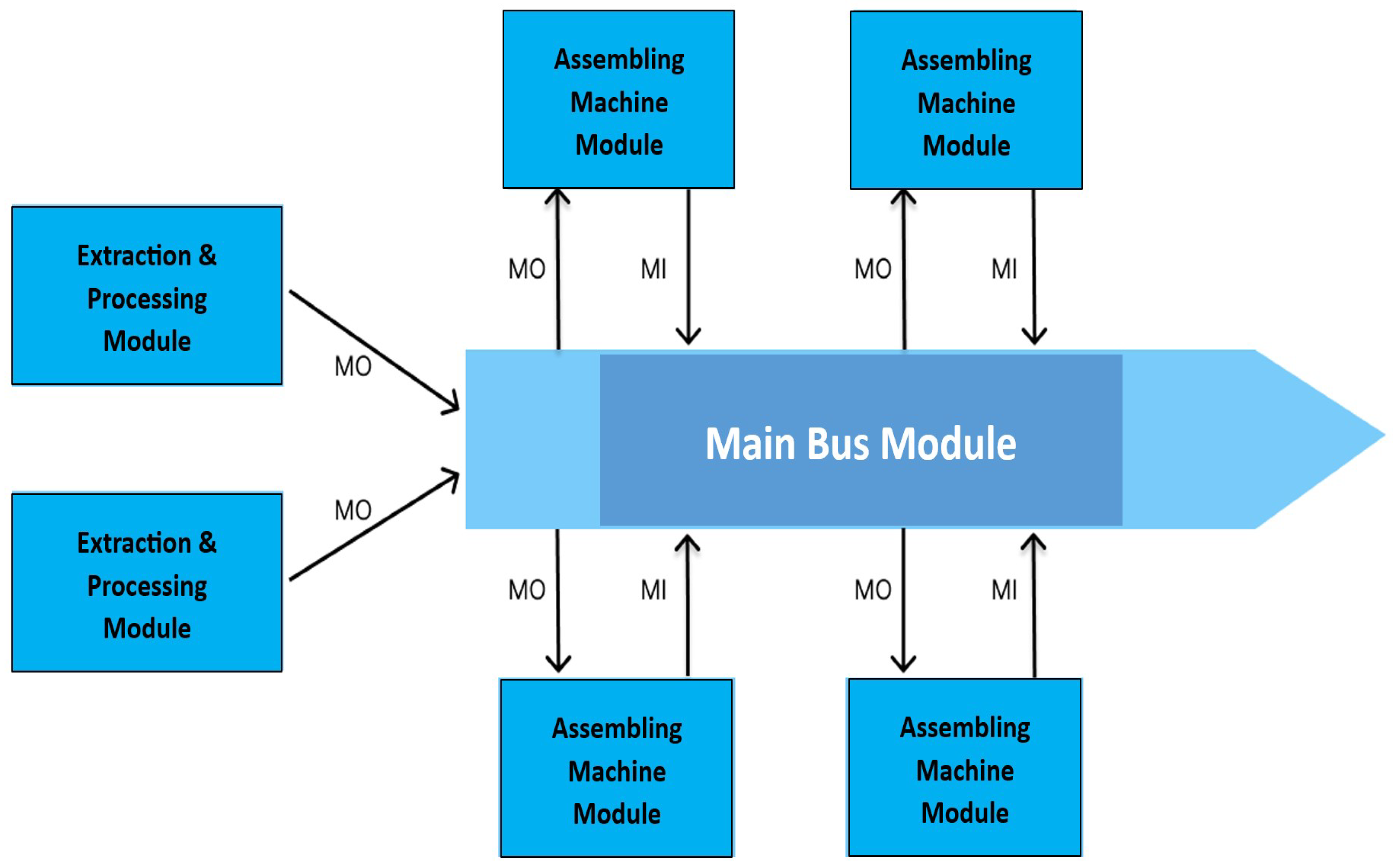
Modeling the Main Bus design system in Factorio can be broken down into discrete, self-contained modules, each responsible for a specific aspect of the production process. By doing so, we aim to enhance our simulation’s scalability and maintainability.

Figure 4 aims to provide an overview of this modular approach. The overview shows the three different types of modules this system incorporates:

• Resource Extraction and Processing Module
• Assembling Machine Module
• Main Bus Module

Additionally, the keywords module-in (MI) and module-out (MO) in Figure 4 detail whether a token is entering or exiting a module.

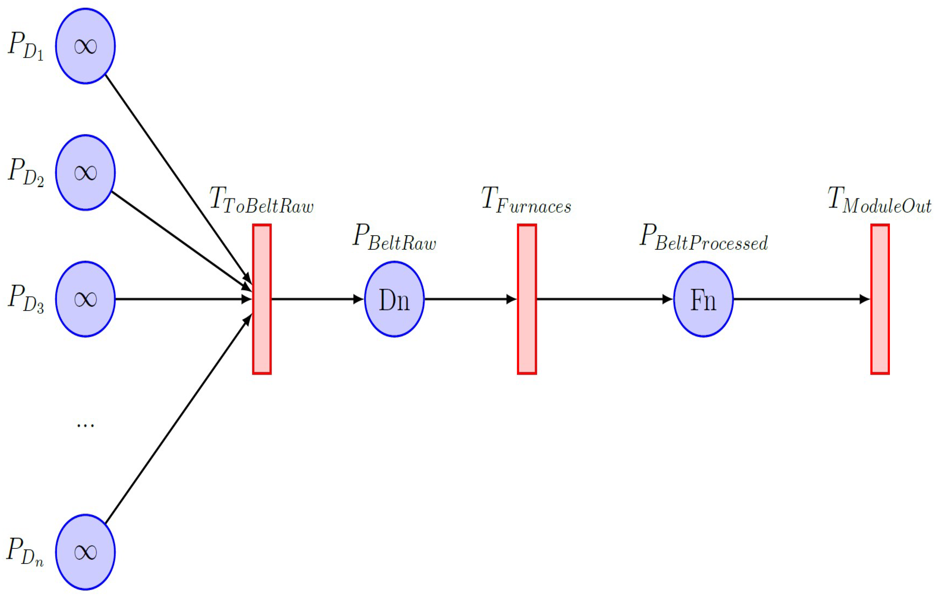
3.2.1. Resource Extraction and Processing Module

This module is dedicated to simulating the processes of raw resource extraction, which include mining minerals using electric drills and initial processing using electrical furnaces. There are various natural minerals in Factorio, but the ones required for our pipeline and this model are Iron Ore and Copper Ore. Modeling this process, we get the Petri Net shown in Figure 5, where $D_n$ and $F_n$ denote the number of electric mining drills and furnaces in our system.

The Petri Module fires one token from $D_n$ places. These places represent mining drills and effectively work as source places, therefore containing ∞ tokens. A source place in Petri Net theory is a special place that has no inbound arcs, only output arcs, and can be assumed to hold infinite tokens. Although this is technically not true for our case, Factorio’s mineral density is sufficient for us to assume it is practically infinite for this paper [15].

Instead of sending the tokens directly into the furnace transitions, additional intermediate steps (conveyor belt places) have been implemented. This is to simulate the Factorio pipeline more accurately and better track the number of tokens at each step, which can be useful for discovering bottlenecks and inefficiencies in our system.

Figure 4. Module overview.

Figure 4. Module overview.

Figure 5. Petri Module for resource extraction and processing.

Figure 5. Petri Module for resource extraction and processing.

The goal of this module is to produce and extract as many resources as possible while being efficient. Efficiency is in the sense of having a balanced ratio between the number of mining drills and furnaces, such that the furnaces consume tokens at the rate the drills generate them. This ensures that we do not end up in a situation where the raw mineral conveyor belt gets congested and reaches its maximum capacity.

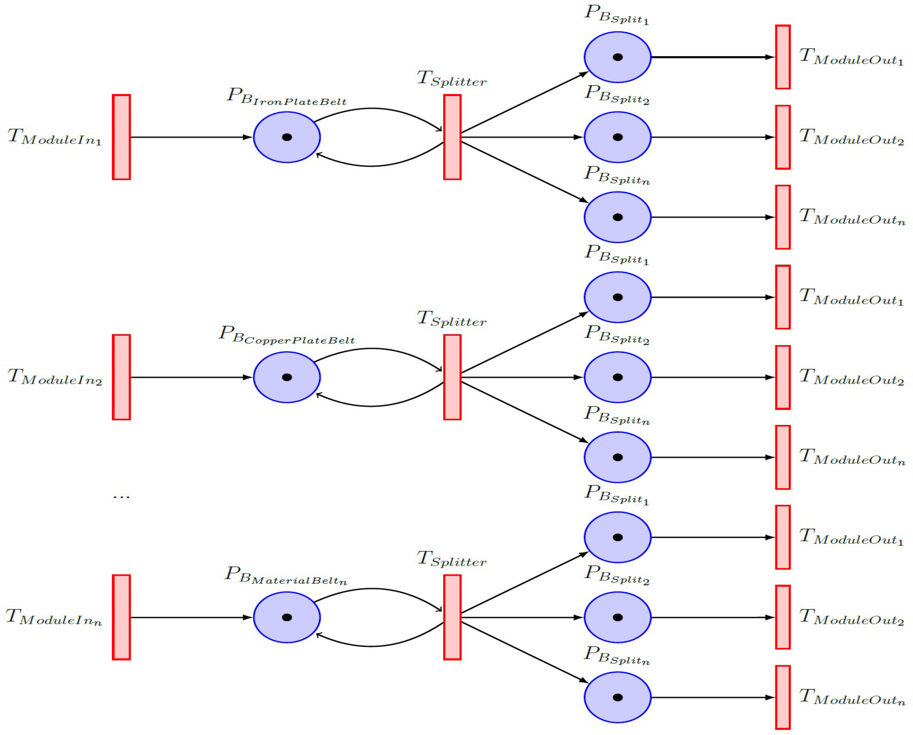
3.2.2. Main Bus Module

The Main Bus module is at the core of our pipeline’s performance and functionality. It is tasked with supplying every other module with its respective materials, and it must work as expected and efficiently. The primary challenge of utilizing a Main Bus design strategy is that it requires a large number of conveyor belts, which may lead to congestion and traffic and, in the worst case, become a logistical nightmare to manage, maintain, and expand.

To best counter these drawbacks, planning your bus before implementing it is vital. This includes figuring out what should be on the bus and what should not, which lanes the various materials should be on, and how much of a material should be on the bus. Figure 6 shows the Petri Net implementation of a Main Bus module where the transition $T_{ModuleI{n}_n}$ is one of the many incoming ports of this module.

Here, the places in the Petri Net model represent various conveyor belts responsible for holding unique items, e.g., iron plates, copper plates, etc. Based on a round-robin approach, the $T_{Splitter}$ transition then decides which next belt the items should be sent to. The final places in this model represent the output belts for this model and have their distinct destination in terms of output ports.

The general idea behind this model is to make it flexible to manage any new addition to the bus without any complications. Splitters divide materials and transport them to different modules where they are needed. They utilize the round-robin method to distribute items between different lanes.

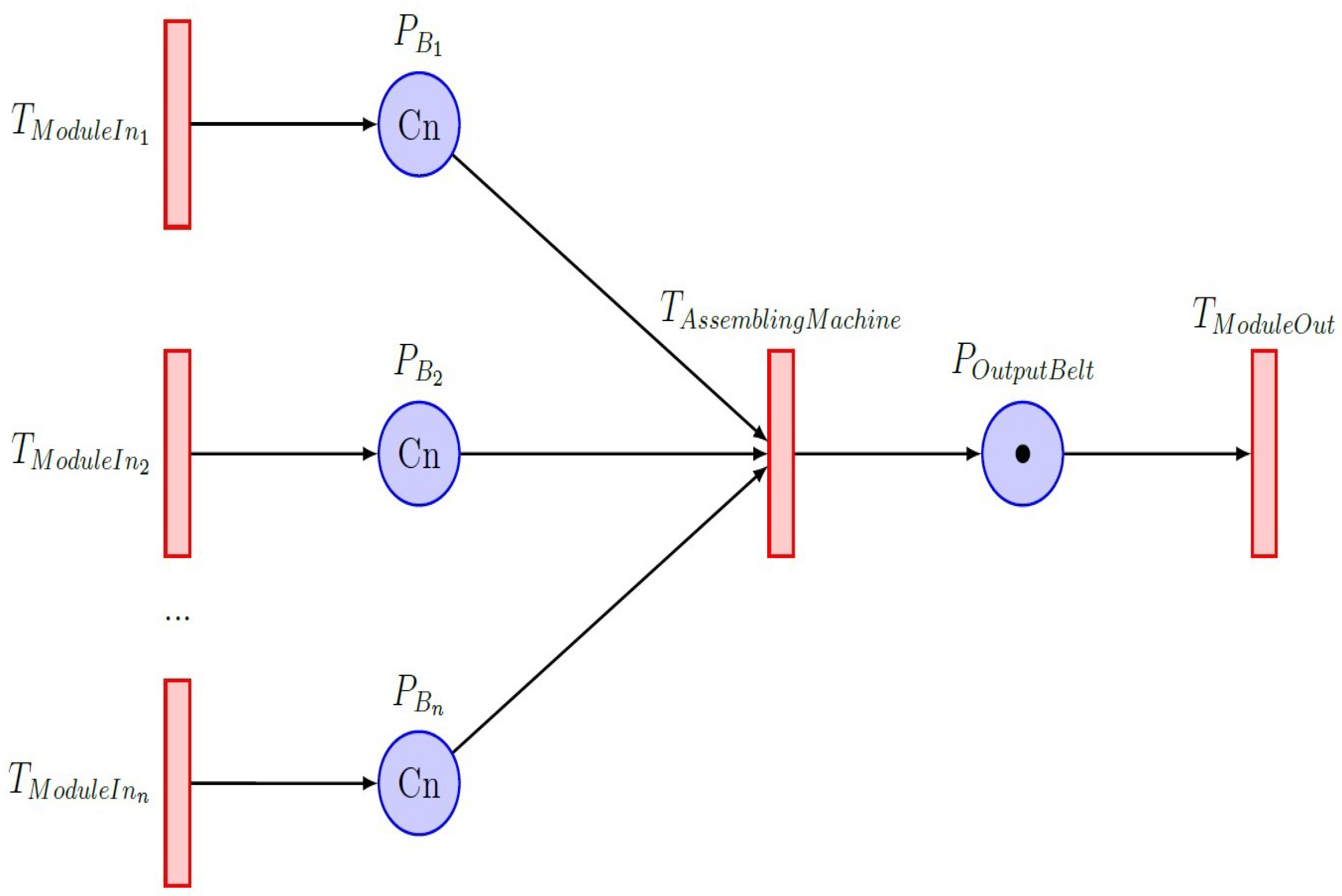
3.2.3. Assembling Machine Module

The last module in our model is the Assembling Machine module, which is responsible for crafting new tokens. This Petri Module can be seen in Figure 7, where $C_n$ denotes the number of materials required for crafting the specific item. The module receives tokens from the Main Bus module via the $T_{ModuleIn}$ transition port. The number of incoming transition ports for this module depends on the number of unique materials in the recipe required for crafting the new item. The crafted item exits the module through the $T_{ModuleOut}$ transition port, eventually reconnecting with the Main Bus.

3.3. Techniques

A Timed Petri Net (TPN) is used to model the pipeline, as Factorio is inherently time-sensitive like many real-world systems. Each machine within the Factorio ecosystem has distinct time requirements to complete its tasks. Therefore, it is important to include time in the model when modeling the behavior of this system.

Table 1. Factorio machine processing times. How many seconds does it take to complete its work, and how many units will be produced?

Machine	Output	Time (s)	Units Produced
Assembling Machine	Iron Gears	0.5	1
Assembling Machine	Copper Cable	0.5	2
Assembling Machine	Conveyor Belt	0.5	2
Assembling Machine	Inserter	0.5	1
Assembling Machine	Electronic Circuit	0.5	1
Electrical Furnace	Smelted Mineral	1.6	1
Electrical Mining Drill	Raw Mineral	2.0	1
Assembling Machine	Automation Science Pack	5.0	1
Assembling Machine	Logistic Science Pack	6.0	1

displays a comprehensive list of all the machines used within the pipeline and their respective run times. The assembling machines’ run times and recipes are gathered from the official Factorio wiki [2], and the run times for the electric mining drill and furnace are calculated using Equation (1).

$$Run\_Time=\frac{Mining\_Productivity\left[\mathrm{units}\right]}{Mining\_Speed\left[\mathrm{units}/\mathrm{s}\right]}$$

(1)

The conveyor belts are implemented with the maximum token capacity to create a realistic simulation. This ensures that the simulated environment resembles the game logic as much as possible. The token capacity for the conveyor belts is calculated using data from the official Factorio Wiki and an approximation of the number of belts required. The simulation includes logic for simulating the splitters’ round-robin distribution.

Finally, energy consumption and pollution costs are measured and evaluated for the different cases. Factorio measures energy consumption in kW and pollution in pollution/min, where pollution is an arbitrary game unit.

Table 2. Factorio machines and their respective costs.

Machine	Energy Consumption (kW)	Pollution (Pollution/min)
Assembling Machine	75	4
Electrical Furnace	180	1
Electrical Mining Drill	90	10

and

Table 3. Factorio Speed Module benefits and costs per unit.

Speed Module	Crafting Speed Increase %	Energy Consumption Increase %
Speed Module 1	20	50
Speed Module 2	30	60
Speed Module 3	50	70

provide an overview of the diverse costs associated with different machines and the effect of equipping machines with varying modules of speed.

4. Implementation

A Modular Petri Net model implemented with GPenSIM generally consists of three groups of files [11]. Hence, the code structure of the Factorio model possesses three groups of files:

• PDFs: All the Petri Net Definitions files for four modules and an Inter-Modular Connector (IMC) named connect_modules_pdf.m. A PDF defines a static Perti Net graph of places, transitions, and arcs.
• Processor Files: Contains both of the common processors, COMMON_PRE and COMMON_POST.
• MSF: The main simulation file (MSF) is responsible for starting and running the simulation.

The files’ codes are not shown in this paper due to brevity. The reader is encouraged to contact the authors for the complete code.

4.1. Main Simulation File (MSF)

The main simulation file does the following:

• Sets the compiler options and initializes the global (global_info) variables and the initial dynamics of the system.
• Sets some specific parameter values (e.g., the maximum token limit for conveyor belts and the number of machines in the pipeline).
• Values for costs in energy consumption and pollution.
• Declares local variables assigned to the sum of each type of machine (these variables are primarily used for calculating costs).
• Declares the new variables and initializes them to store results and scores.
• Confgiures Machine_configurations variables for carrying info about the effects of speed modules (see Table 3).
• Assigns firing times for all the transitions in the Petri Net.

4.2. Processor Files

The COMMON_PRE and COMMON_POST files serve distinct roles in pre- and post-processing logic for transitions, responsible for actions taken before and after a transition is fired. Specifically, COMMON_PRE is responsible for ensuring that conveyor belts do not exceed their maximum token capacity, and both COMMON_PRE and COMMON_POST are responsible for enforcing the round-robin distribution of splitters.

We first consider the implementation of the pre-processing file COMMON_PRE. In COMMON_PRE,

• The logic allows enabled transitions to fire unless the incoming belt has reached its capacity (in this case, the transition id prevented from firing).
• The round-robin distribution logic is implemented for checking the belt capacity (if the incoming belt is at max capacity, it will increment the global variable such that another transition can fire instead).

COMMON_POST will run after a transition fire:

• Changes the global toggle variable if the transition incorporates the splitter logic.

5. Simulations, Analysis, and Optimization

This section covers multiple simulation runs involving different pipeline configurations. We briefly discuss the results, explore methods of determining scoring pipelines, and optimize our parameters based on the results.

5.1. Exploring Scoring Functions

Before running a series of simulations to determine the most optimal pipeline, we need to establish what an optimal pipeline would look like. The following list outlines a set of criteria the pipeline needs to consider for it to be optimal:

• Maximize the number of total science pack tokens (red and green science packs).
• A healthy ratio between red and green science packs. It should be close to 50/50.
• Minimize energy consumption (EC).
• Minimize pollution (Pol).

The following equation attempts to score a simulation run based on the abovementioned criteria, where $w_1$ and $w_2$ are weight parameters.

$$f\left(score\right)=\frac{\left(S{P}_t\right)·\left(\frac{min\left(SP\right)}{max\left(SP\right)}\right)}{w_1\frac{EC}{S{P}_t}+w_2\frac{Pol}{S{P}_t}}$$

(2)

$$S{P}_t=\sum _{i=1}^{k}S{P}_i,\mathrm{SP}=\left\{\mathrm{red\; science\; pack,\; green\; science\; pack}\right\}$$

(3)

For a pipeline to maximize its score, it needs to maximize the numerator and minimize the denominator. The numerator represents the total number of science packs produced times its ratio. The ratio will always be a number between $[0–1]$ and is maximized by having a 50/50 ratio. The denominator is minimized by having as low as possible pollution and energy consumption per science pack produced. Weight parameters $w_1$ and $w_2$ can be adjusted according to our specific system’s energy consumption and pollution importance.

Additionally, individual metrics such as energy consumption, pollution, and science pack production are stored and plotted for manual inspection.

5.2. Simulation Run with Arbitrary Parameters

Before our first simulation run, we need to determine what our parameters should be. Without prior knowledge of the most effective configurations for our parameters, we rely on intuition, common sense, and data available on the Factorio wiki [2]. The goal is to select realistic parameters for our simulation run and use them as a baseline to be further optimized.

Parameter Configuration Details

The parameters we need to define are the number of electric mining drills for copper and iron ore. Utilizing data from Table 1,

Table 4. Factorio science pack crafting recipes [2].

Output	Copper Plate	Iron Gears	Inserter	Conveyor Belt
Red Science Pack	1	1	0	0
Green Science Pack	0	0	1	1

, and

Table 5. Factorio science pack crafting recipe raw materials [2].

Output	Copper Plate	Iron Plate
Red Science Pack	1	2
Green Science Pack	1.5	5.5

, we can make a realistic assumption about what these numbers should be. Table 4 shows the ingredients required for crafting the red and the green science packs, while Table 5 shows the raw ingredients, as in iron and copper plates.

Based on the data displayed in the raw materials table, we require more iron plates than copper plates in our production pipeline. Inspecting Table 1, showing the time required for each machine, we also see that each furnace only uses 1.6 s compared to the 2.0 s the mining drills use. Based on this information, we can assume that the number of furnaces should be less than that of mining drills as they produce faster. The same table also displays the time required for the various assembling machines and how many units they produce. All these factors are taken into account to produce the parameters shown in

Table 6. Pipeline parameter configuration.

Machine	Amount
nIron_Electric_Mining_Drills	25
nCopper_Electric_Mining_Drills	20
nIron_Electric_Furnaces	20
nCopper_Electric_Furnaces	15
nAM_Iron_Gear	10
nAM_Copper_Cables	5
nAM_RSP	5
nAM_Electric_Circuit	10
nAM_Inserter	10
nAM_Conveyor	5
nAM_GSP	5

.

This arbitrarily high number of mining drills is set such that we ensure that it produces enough raw materials to supply the pipeline with items downstream sufficiently. The remaining parameters are set based on their production rate compared to the output of the drills and furnaces. In other words, we employ a naive strategy of having a high production rate by having many machines.

Additionally, parameters like time step and total running time are set to 0.1 and 120, respectively. Due to the deterministic features of our system, we can assume any trends will hold for the future. Therefore, a 120-s run time for our simulation will suffice. Both time step and allothers transition times are set to 0.1. This is effectively the belt throughput speed of our pipeline, i.e., $belt\_throughput=10$ items/s.

5.3. Simulation Results

After setting the initial parameters, it is time to run the simulation to explore how our pipeline performs under the chosen configurations. This section comprehensively analyzes key metrics, including production rates, energy consumption, and pollution levels. The outcomes of this simulation serve as a baseline for comparison against optimized parameters in the subsequent section.

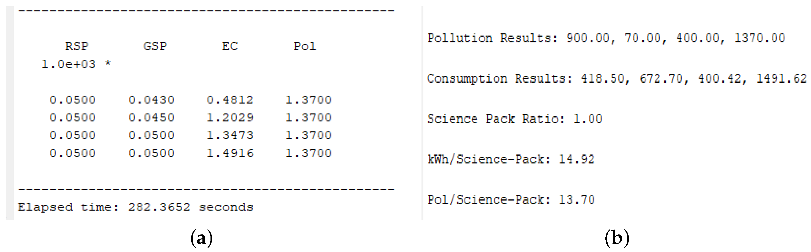
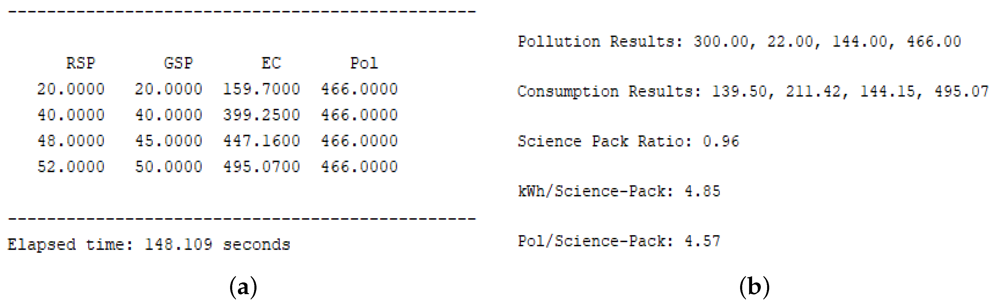
Figure 8 shows performance metrics generated by the simulation.

Figure 8a shows the data generated by all four simulation runs, from not using a speed module to speed module 3. It captures the most important metrics, such as:

• Red science pack tokens produced.
• Green science pack tokens produced.
• Total energy consumption for all machines.
• Total pollution from all machines.

Figure 8b shows performance metrics calculated based on the simulation, such as energy consumption/pollution per science pack, total costs and the ratio between science packs. These numbers can then be used to calculate a score using the custom scoring function described previously in Equation (2).

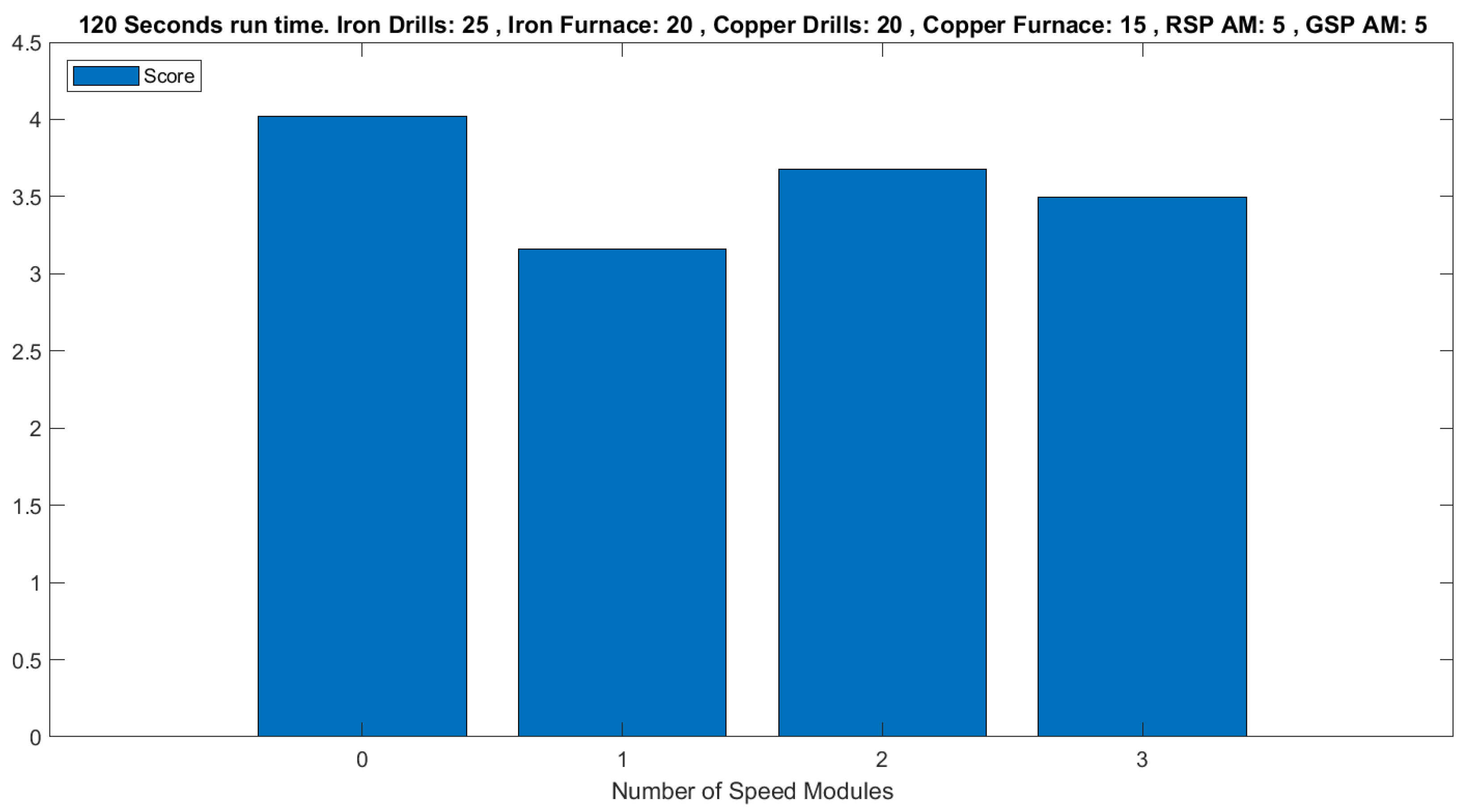
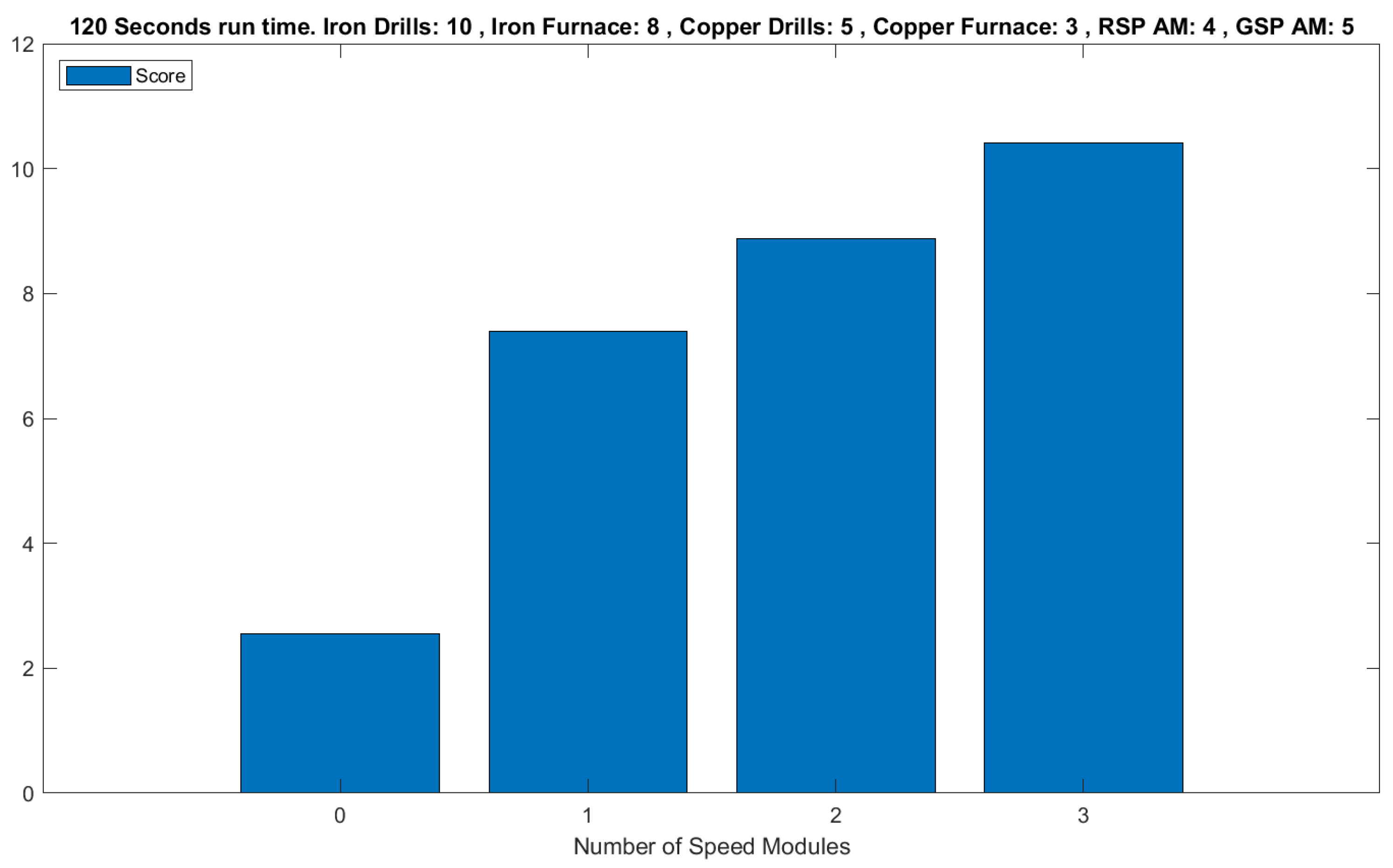
Figure 9 shows our pipeline’s score for each Factorio speed module configuration. The $w_1$ and $w_2$ weight parameters were set to 1, placing equal importance on energy consumption and pollution.

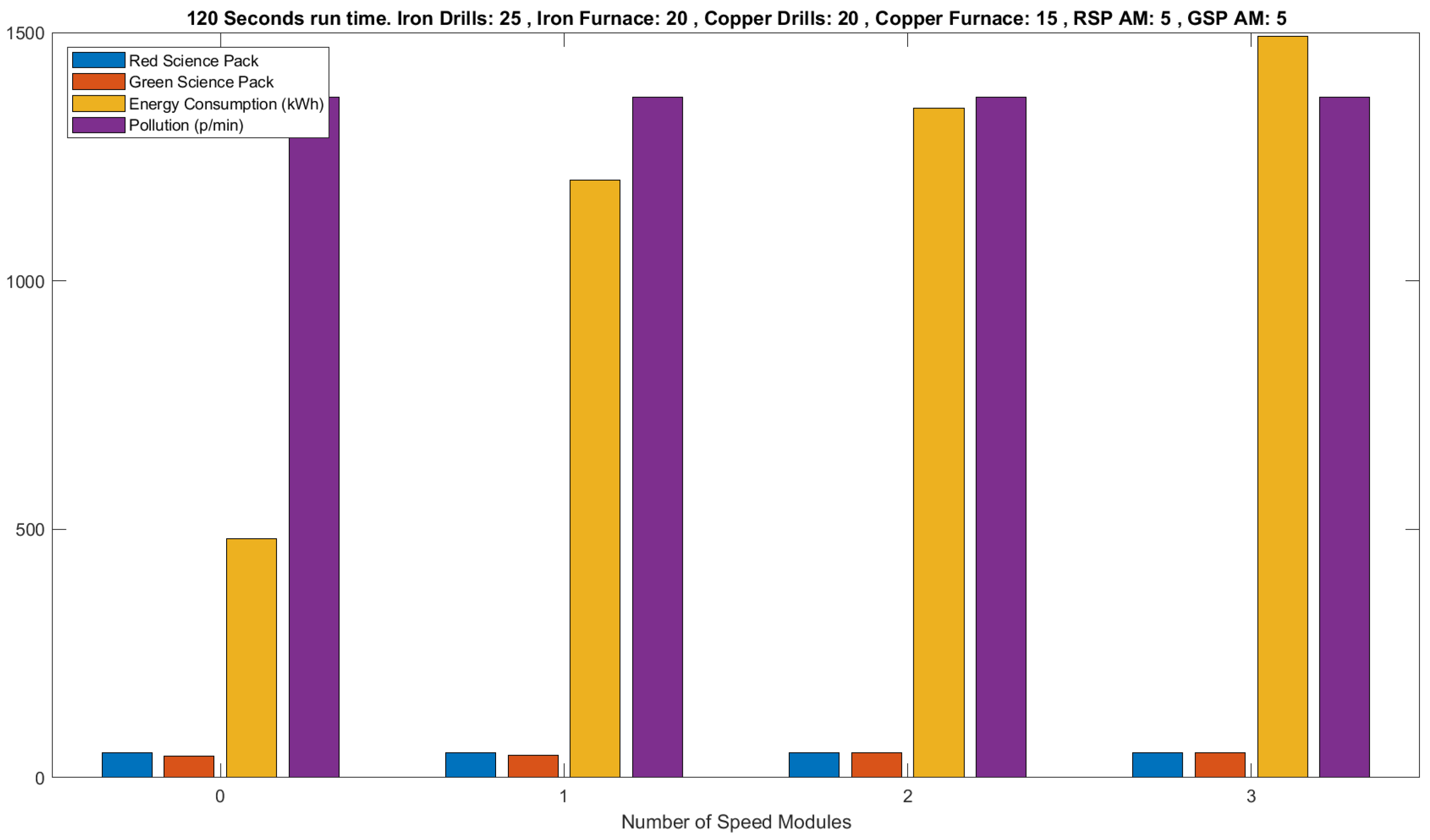
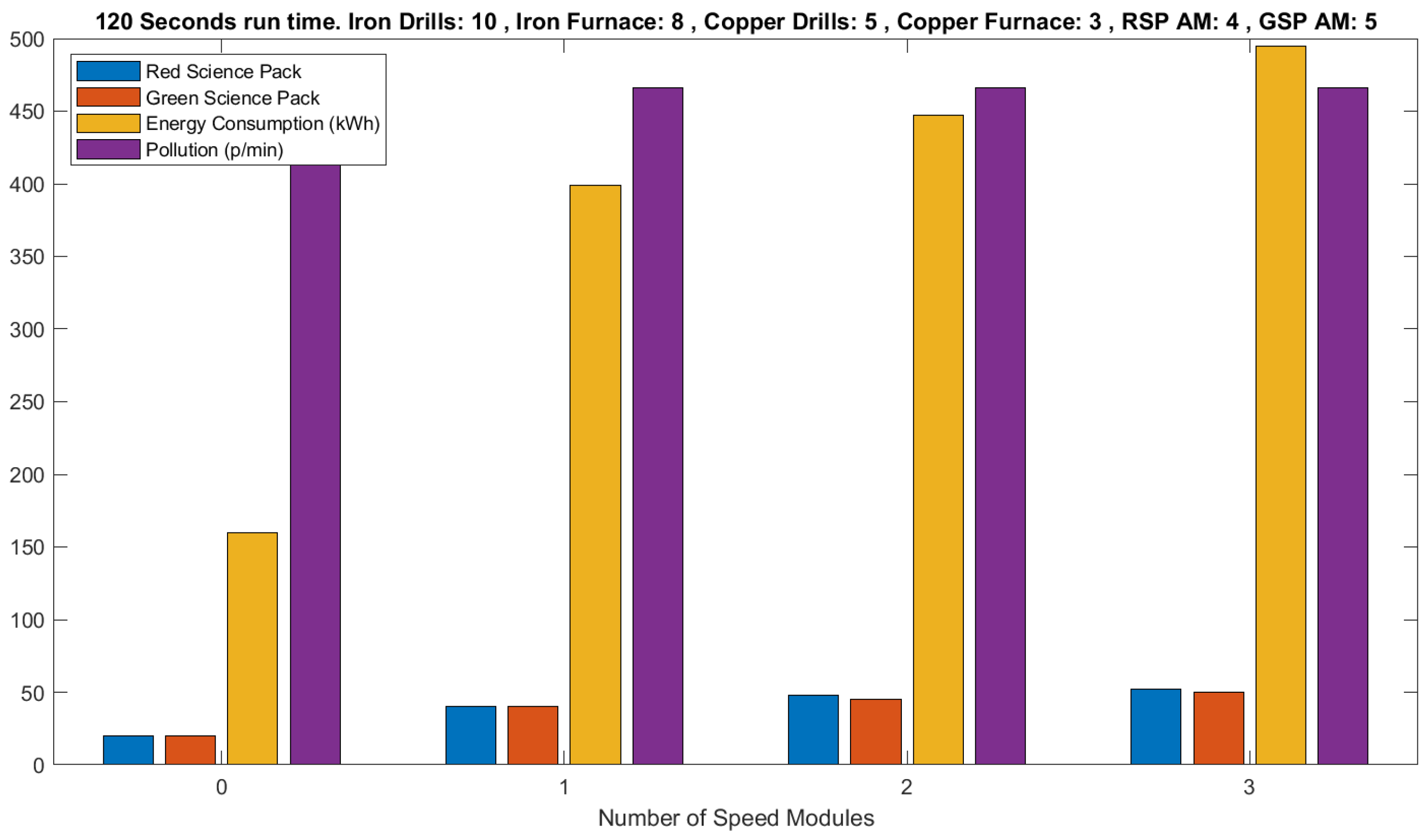
From the bar plot displaying the scores, we see that the pipeline configuration that performs the best is the one without any speed modules. Looking closer at the raw performance metrics shown in Figure 10, we can see science pack production against its costs for the different speed module configurations.

Analyzing Results

It is obvious from the raw performance metrics that the insertion of speed modules does not effectively increase science pack production. Although it increases production slightly, energy consumption skyrockets. Looking at Figure 10, it makes sense that the pipeline configuration with zero speed modules scores best given the lower energy demand. Table 3, displaying speed module data, describes a 50% speed increase per speed module per unit. This increase in production is not seen in this simulation run. Notably, pollution remains constant across each simulation run as speed modules do not affect pollution.

Figure 9. Scores between different speed module configurations for the pipeline.

Figure 9. Scores between different speed module configurations for the pipeline.

Figure 10. Raw performance metrics bar plot.

Figure 10. Raw performance metrics bar plot.

5.4. Simulation Run with Optimized Parameters

Previous findings show a rather lacking production increase from the insertion of speed modules into our machines. This section explores why that is and attempts to rectify it.

5.4.1. Exploring Potential Bottlenecks

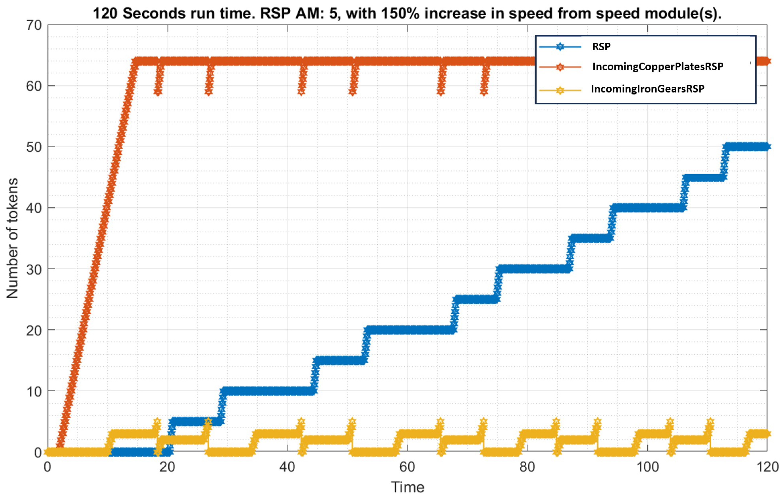
We start our investigation by looking at the last production modules in our pipeline, namely, the red and green science pack modules. Figure 11 shows the number of tokens in each place of the red science pack module throughout the simulation.

In this module, we see a sharp increase in incoming copper plate tokens until it reaches a maximum capacity of 64 at around 17 s and steadily maintains the same amount of tokens throughout the simulation. Although the red science pack tokens increase, the time interval at which it does is uneven. Given sufficient supply, it will take $\frac{5 \mathrm{s}}{2.5}=2 \mathrm{s}$ for the assembling machine to produce tokens, given it has three speed modules inserted. This simulation produced the output in intervals of 8.5 and 15.5 s, meaning it has an average production time of 12 s. From inspecting the plot, we see that the lack of incoming iron gear tokens is the reason for this poor production rate.

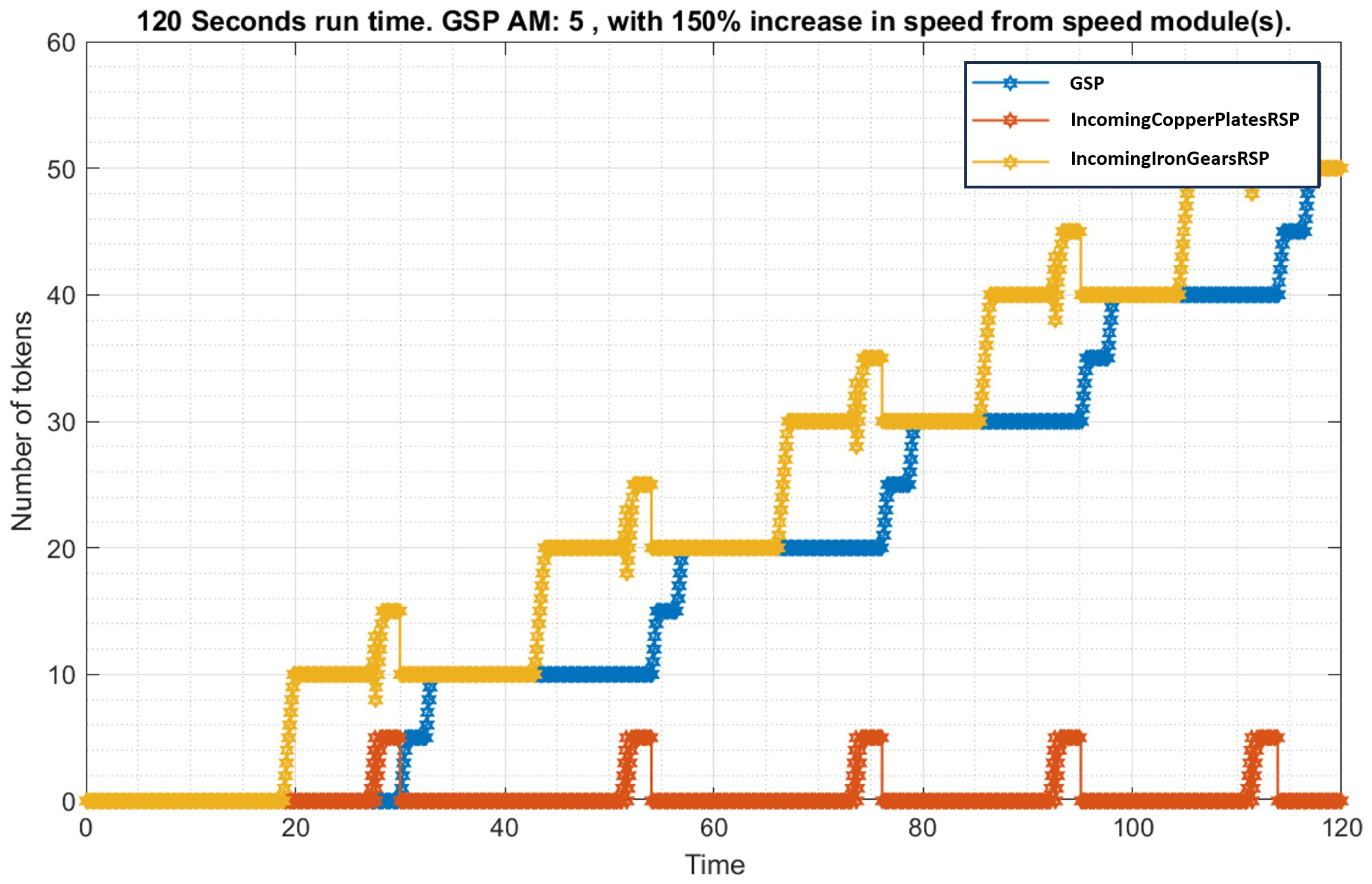
Figure 12 shows the token amount for the various places in the green science pack module.

Figure 12 shows a problem similar to the red science pack module. The number of incoming conveyor belt tokens increases until it reaches the maximum token capacity at around 77 s. However, the insufficient supply of incoming inserter tokens severely halts the production of green science pack tokens, as can be seen from the time intervals it produces. The production of green science pack tokens is more time-consuming, takes 6 s base, and is expected to take $\frac{6 \mathrm{s}}{2.5}=2.4$ with three speed modules inserted. The time intervals for this simulation are 2.5 and 16.3 s, meaning it takes an average of 9.4 s.

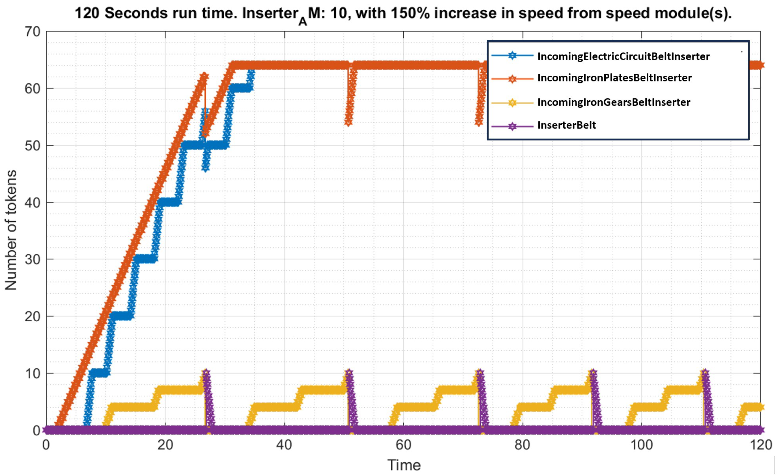
As the problem seems to lie with the supply of inserter tokens, we take a closer look at the inserter module to see what is slowing down the production. The number of tokens at each place for the inserter module displayed in Figure 13 shows that it also lacks iron gear tokens. The inserter module can theoretically produce tokens every $\frac{0.5 \mathrm{s}}{2.5}=0.2$ s, but only produces tokens on average every $\approx 20$ s.

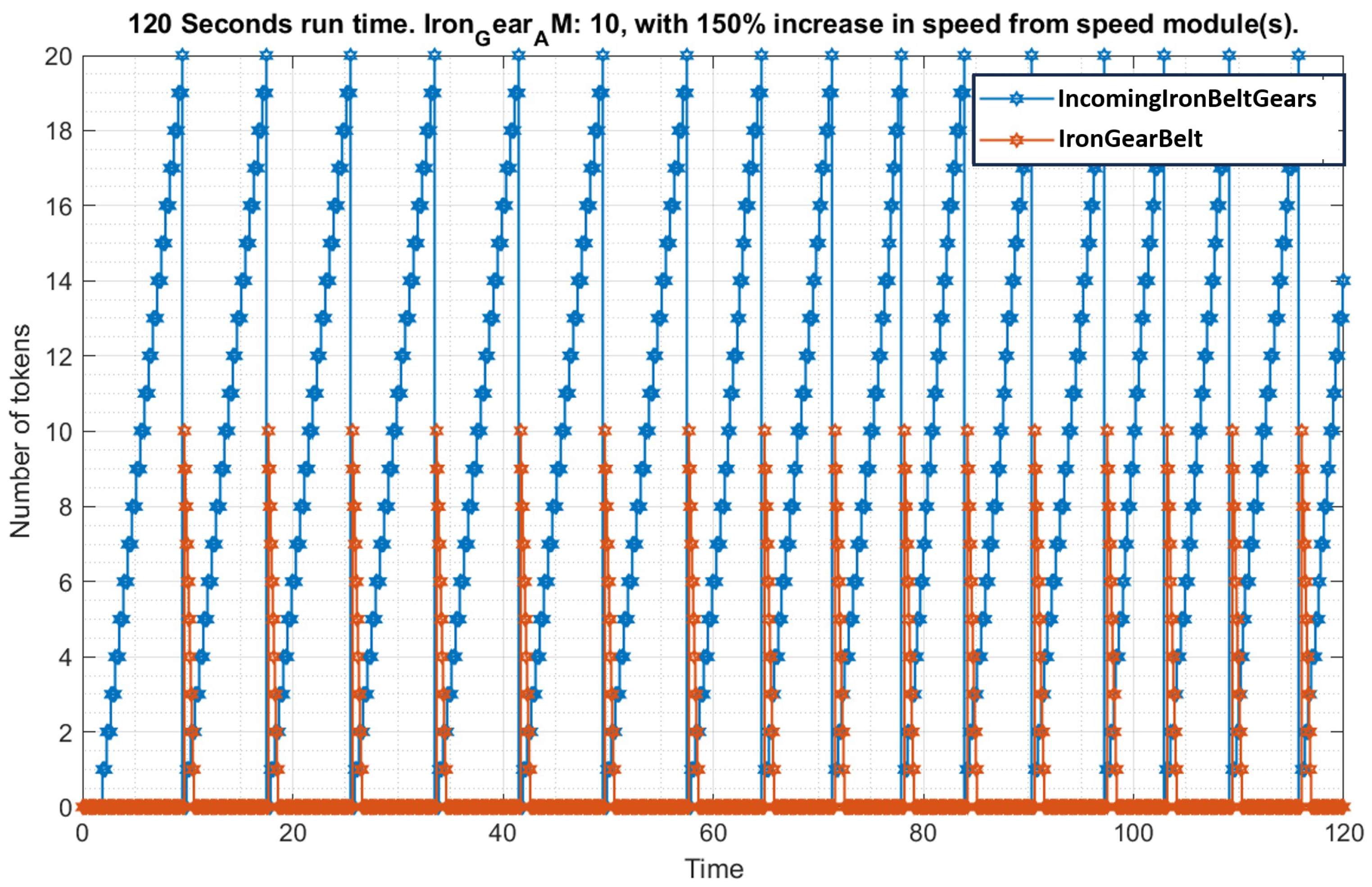
Figure 14 shows the token count of the incoming iron plate place and the outgoing iron gear place for the iron gear module. The plot shows that it produces ten iron gear tokens within even time intervals of around 8 s. Still, the iron gear module can produce tokens every 0.2 s with sufficient resources.

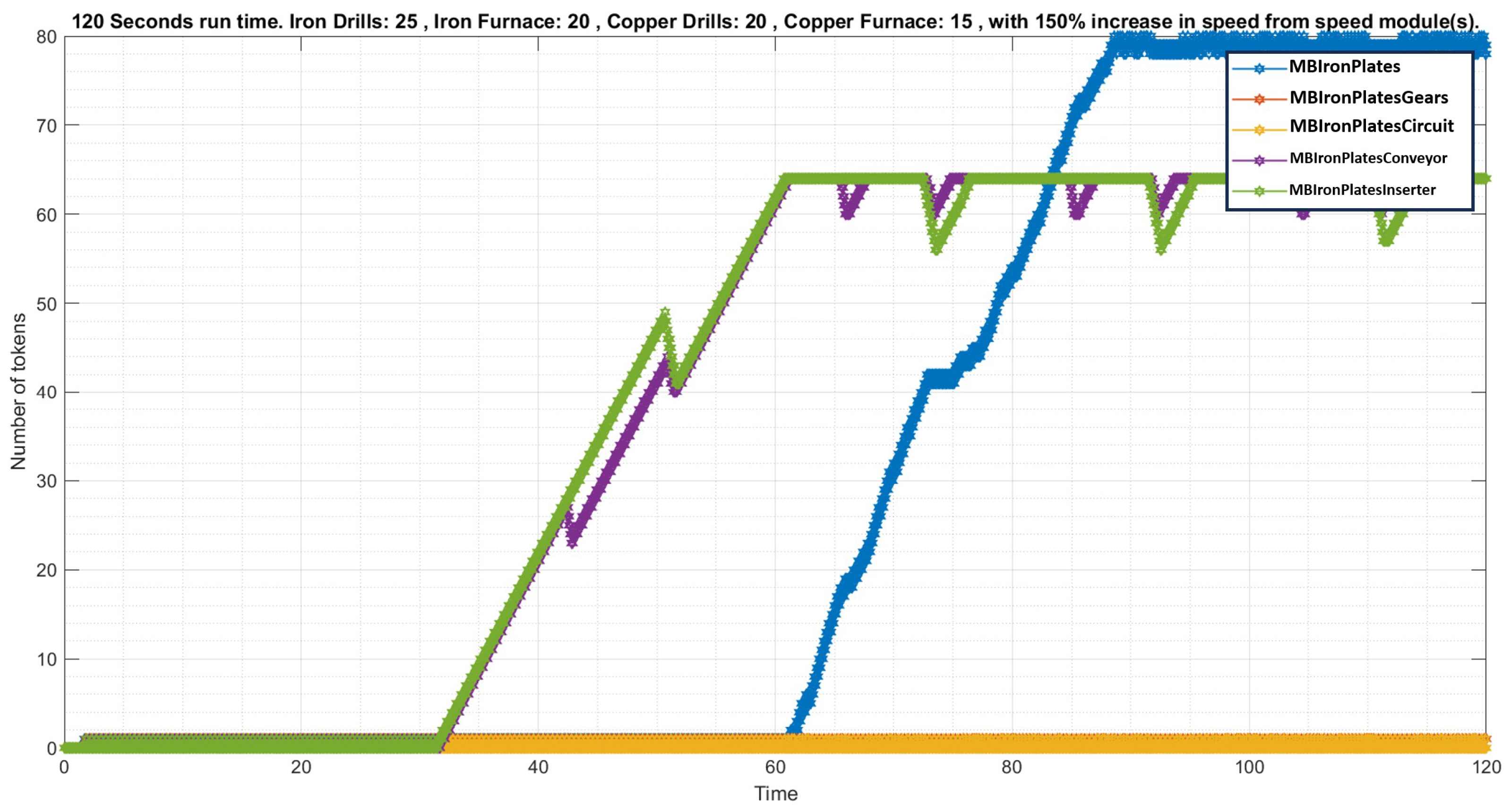
Figure 15 shows the iron plate belt places from the Main Bus module. As with the other modules, we see increases in other items except for the iron gear and electric circuit place. This suggests that we lack sufficient iron plate production.

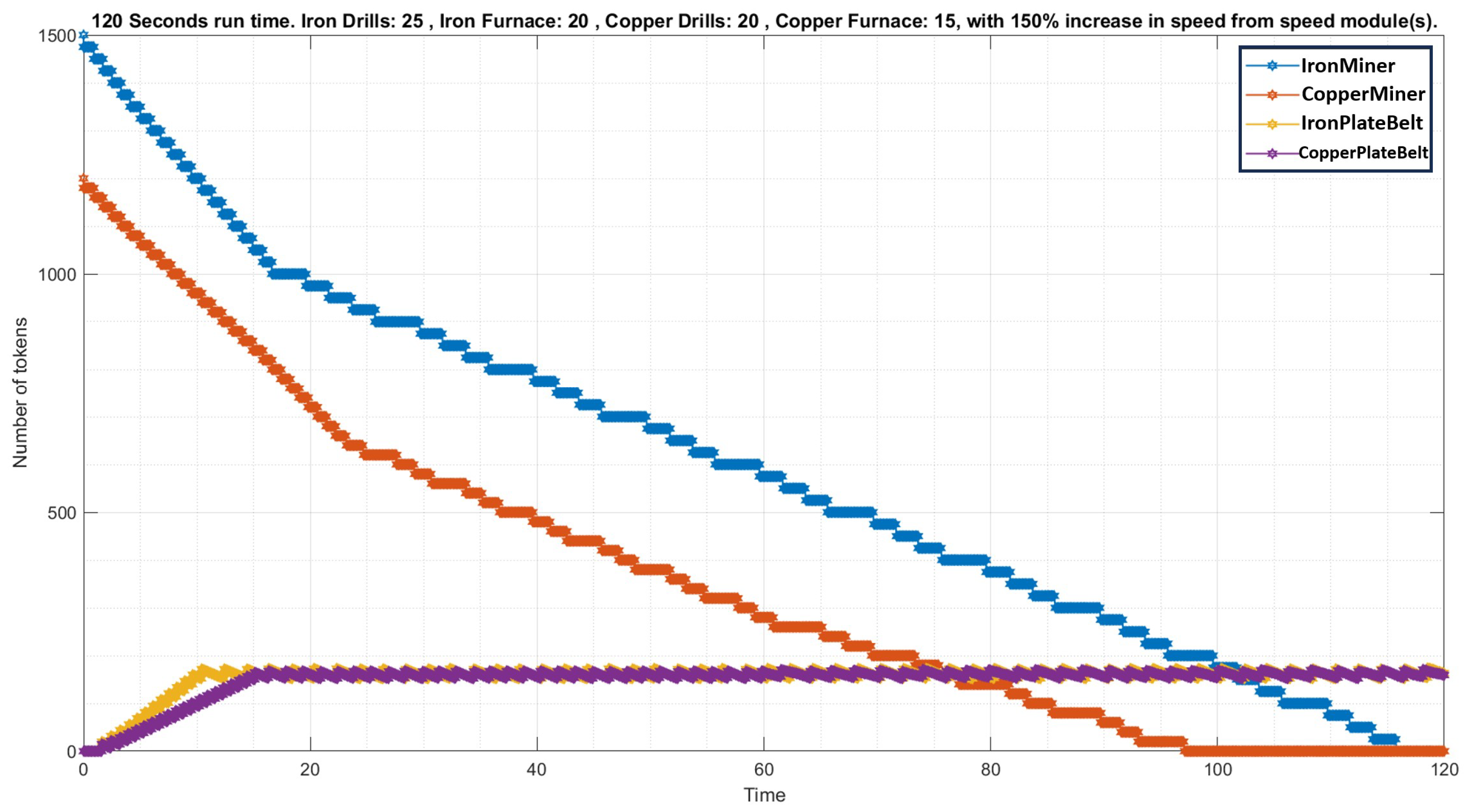
Figure 16 shows the token count for places in the resource extraction module. After about 10–15 s of running our simulation, we have reached a maximum capacity of 160 tokens for the output belt for both copper and iron.

Based on the information gained from the token-place plots of the various modules in our pipeline, several issues keep our system from being optimal. These issues are as follows:

• Overproduction in the resource extraction modules: The mining drills and furnaces produce more tokens than the conveyor belts can throughput.
• Excessive assembling machines. The supply is insufficient to justify the number of machines assembled, or the machines are overproducing.

5.4.2. Parameter Optimization

In this section, we aim to address the issues detailed in the previous section. The optimization strategy for this pipeline is twofold: first, we aim to reduce the number of machines in the resource extraction module to better align the throughput of the conveyor belt. Second, we aim to adjust the number of assembling machines to better align with the available supply of tokens for each module.

Table 7. Optimized pipeline parameter configuration.

Machine	Amount
nIron_Electric_Mining_Drills	10
nCopper_Electric_Mining_Drills	5
nIron_Electric_Furnaces	8
nCopper_Electric_Furnaces	3
nAM_Iron_Gear	2
nAM_Copper_Cables	1
nAM_RSP	4
nAM_Electric_Circuit	3
nAM_Inserter	2
nAM_Conveyor	1
nAM_GSP	5

shows the parameter values.

5.4.3. Optimized Simulation Results

Simulating with our new optimized parameters yields numerical results as shown in Figure 17.

We see greatly reduced costs in terms of both energy consumption and pollution. This, in turn, results in reduced energy consumption and pollution per science pack. We also see a healthy ratio between red and green science packs. The numbers from our simulation are used to score our pipelines using the same weights and give us Figure 18.

We see from the bar plot displaying the scores that the pipeline configuration that performs the best is the one using three speed modules. Figure 19 shows our pipelines’ raw performance metric score with the new configurations.

Based on the results from the Figure 18 and Figure 19, it is a clear improvement from our earlier naive pipeline.

5.5. Data Description

All the data used in this simulation, such as the recipes, number of output tokens, and transition times, are all from the official Factorio Wiki [2]. There is, however, an adjustment made to the original Factorio data, namely, a change to the belt throughput speed, which is officially set at 15 items/s, compared to our 10 items/s [16]. This change is done due to simplicity. It is easier to work with and analyze 0.1 as the time step than 0.666.

5.6. Final Remarks

Table 8. Overview of different system configurations.

Configuration	Minimum	Average	Maximum
Optimized	2.5	7.3	10.4
Arbitrary	3.2	3.6	4.0

provides an overview of the two different system configurations regarding the score.

Table 8 shows that there is a 100% increase in the average score going from the arbitrary pipeline configuration to the optimized pipeline configuration.

6. Discussion

The work presented in this paper is novel in that we use Modular Petri Nets to model the game scenario and GPenSIM for implementation. Modular modeling allows the extension or alternation of individual modules without affecting the rest of the model. Also, modules (Petri Modules) implemented with GPenSIM can be run on geographically distributed computers, enhancing model development by different development groups and increasing the simulation speed (as simple and lightweight Petri Modules are run on computers). Also, GPenSIM is a toolbox on MATLAB; as such, it allows Petri Net models to use the functions available in numerous MATLAB toolboxes seamlessly.

The game scenario of Factorio is fundamentally a discrete-event system. Hence, several modeling formalisms and methodologies (such as Markov Chains, Automata, SimEvnts, and StateFlow) can be used. We chose Petri Nets because of its favorable properties, such as self-documentation, simple mathematical background, and explicit state information (reachability tree) [9]. However, modeling a game scenario of Factorio would result in a huge Petri Net, causing a state explosion in the reachability tree analysis. For this reason, we chose Modular Petri Nets, composed of manageable (smaller) Petri modules [10].

6.1. Limitations of This Paper

The modeling and simulation presented in this paper contain some simplifications and approximations applied to certain aspects of the game, including the approximation of the conveyor belt throughput. Additionally, the system is configured such that an assembling machine only fires if all assembling machines are within the same module. In Factorio, an assembling machine will automatically start producing if it has the required resources regardless of other machines.

6.2. Further Work

In this paper, we have not discussed verification of the Petri Net model. This is because the Petri Net model we present in this paper is a modular Petri Net composed of Colored Petri Modules. Literature studies reveal some attempts to verify Colored Petri Nets; there are also some attempts to verify modular Petri Nets. However, no research has been done on verifying modular Petri Nets composed of Colored Petri Modules. Also, the scope and focus of this paper are limited to show that it is possible to create a Petri Net that can function as a model for the strategic choices we make in a game scenario and then compare the different scores to choose the optimal pipeline configuration. The verification of the model can be taken as further work of this paper.

Another proposal for further work is to expand the Factorio pipeline, including more items for the production line, including all game modules [17]. Factorio also has three different types of assembling machines, while this paper only focuses on one assembling machine [18]. Including costs other than energy consumption and pollution, such as area usage, would be interesting as it encompasses a different objective for players to maximize the outcome.

6.3. Practical Implication

The practical implication of this paper is that the Petri Net model can function as an expert system for the gamer to consult his strategic moves.

References

- Bonnie, S.; Boardman, C.C.K. Simulation of Production and Inventory Control using the Computer Game Factorio. In Proceedings of the 2021 ASEE Gulf-Southwest Annual Conference Baylor University, Waco, TX, USA, 24–26 March 2021. [Google Scholar]
- Official Factorio Wiki. Available online: https://wiki.factorio.com/ (accessed on 3 March 2024).
- Hoffmann, R. Towards Automatic Design of Factorio Blueprints. arXiv 2023, arXiv:2310.01505. [Google Scholar]
- Reid, K.N. The Factory Must Grow: Automation in Factorio. In Proceedings of the Genetic and Evolutionary Computation Conference Companion, Lille, France, 10–14 July 2021. [Google Scholar]
- Leue, A. Verification of Factorio Belt Balancers Using Petri Nets. 2021. Available online: https://d-nb.info/123465766X/34 (accessed on 3 March 2024).
- Colombo, C.; Pace, G.J. Linear Temporal Logic. In Runtime Verification: A Hands-On Approach in Java; Springer International Publishing: Cham, Switzerland, 2022; pp. 109–122. [Google Scholar] [CrossRef]
- Neumann, R. Using Promela in a Fully Verified Executable LTL Model Checker. In Verified Software: Theories, Tools and Experiments; Giannakopoulou, D., Kroening, D., Eds.; Springer International Publishing: Cham, Switzerland, 2014; pp. 105–114. [Google Scholar]
- Murata, T. Petri nets: Properties, analysis and applications. Proc. IEEE 1989, 77, 541–580. [Google Scholar] [CrossRef]
- Peterson, J.L. Petri Net Theory and the Modeling of Systems; Prentice Hall PTR: Upper Saddle River, NJ, USA, 1981. [Google Scholar]
- Davidrajuh, R. Petri Nets for Modeling of Large Discrete Systems; Springer: Berlin/Heidelberg, Germany, 2021. [Google Scholar]
- Davidrajuh, R. Modeling Discrete-Event Systems with GPenSIM; Springer International Publishing: Cham, Switzerland, 2018. [Google Scholar] [CrossRef]
- GPenSIM. General-Purpose Petri Net Simulator. Technical Report. 2019. Available online: http://www.davidrajuh.net/gpensim (accessed on 20 July 2020).
- Davidrajuh, R. Colored Petri Nets for Modeling of Discrete Systems: A Practical Approach with GPenSIM; Springer Nature: Berlin/Heidelberg, Germany, 2023. [Google Scholar]
- Factory. Factorio Wiki—Main Bus Design. 2020. Available online: https://wiki.factorio.com/Tutorial:Main_bus (accessed on 3 March 2024).
- Halder, A. A Study of Petri Nets. 2006. Available online: https://abhishekhalder.bitbucket.io/PetriNetReport.pdf (accessed on 3 March 2024).
- Software, W. Factorio Wiki-Belts. 2022. Available online: https://wiki.factorio.com/Transport_belt (accessed on 3 March 2024).
- Software, W. Factorio Wiki-Modules. 2021. Available online: https://wiki.factorio.com/Module (accessed on 3 March 2024).
- Software, W. Factorio Wiki-Assembling-Machines. 2020. Available online: https://wiki.factorio.com/Assembling_machine (accessed on 3 March 2024).
Figure 1.
Table showing the various science packs and materials required for crafting [
2].
Figure 3.
Mining drill furnaces—assembling machines—Main Bus expansion.
Figure 6.
Petri Module for the Main Bus.
Figure 7.
Petri Module for the Assembling Machine.
Figure 8.
Data generated by running the simulation. (a) Command Window Output (1). (b) Command Window Output (2).
Figure 11.
Arbitrary parameter simulation run: red science pack module.
Figure 12.
Arbitrary parameter simulation run: green science pack module.
Figure 13.
Arbitrary parameter simulation run: inserter module.
Figure 14.
Arbitrary parameter simulation run: iron gear module.
Figure 15.
Arbitrary parameter simulation run: Iron plate belt module.
Figure 16.
Arbitrary parameter simulation run: resource extraction module.
Figure 17.
Data generated by running the simulation (Optimized). (a) Command Window Output (1 Optimized). (b) Command Window Output (2 Optimized).
Figure 18.
Optimized parameter simulation run: scores.
Figure 19.
Optimized parameter simulation run: raw performance metrics.