Abstract
Online fashion retailers face enormous challenges due to high return rates that significantly affect their operational performance. Proactively predicting returns at the point of order placement allows for preemptive interventions to reduce potentially problematic transactions. We propose an innovative inductive Heterogeneous Graph Neural Network tailored for proactive return prediction within the realm of online fashion retail. Our model intricately encapsulates customer preferences, product attributes, and order characteristics, providing a holistic approach to return prediction. Through evaluation using real-world data sourced from an online fashion retail platform, our methodology demonstrates superior predictive accuracy on the return behavior of repeat customers, compared to conventional machine learning techniques. Furthermore, through ablation analysis, we underscore the importance of simultaneously capturing customer, order, and product characteristics for an effective proactive return prediction model.
1. Introduction
In recent years, online fashion retail has experienced substantial growth worldwide, with the global market reaching a value of approximately 820 billion U.S. dollars in 2023, as reported by Statista.com (https://www.statista.com/topics/9288/fashion-e-commerce-worldwide/#topicOverview (accessed on 4 January 2024)). To enhance customer convenience and satisfaction, many online retailers offer free shipping and hassle-free returns. However, this customer-friendly policy results in a significant increase in return rates. This poses a considerable challenge for online fashion retailers as it can severely impact their operational performance. The estimated rate of return for online retailers is typically two to three times higher than that of traditional brick-and-mortar stores, with online fashion retailers experiencing return rates as high as 50% [1]. These frequent returns result in considerable additional costs for online fashion retailers, including expenses related to transportation, reorganizing, and checking, thereby significantly undermining their overall performance.
Product returns also represent a significant contributor to the carbon footprint of e-commerce, due in part to the high energy consumption inherent in the ‘last mile’ of the delivery chain that brings products directly to customers’ doorsteps [2]. Addressing the issue of product returns can thus have substantial implications for the sustainability of e-commerce, not only in terms of ecological impact but also from an economic perspective [1].
One potential strategy for reducing return rates in online fashion retail involves implementing a proactive prediction model within the ordering system to anticipate potential returns at an early stage, prior to order placement. When a customer assembles a purchasing basket, such a model can generate return predictions for each product included in the basket. If the predicted probability of return for a product surpasses a predefined threshold, the system can take preemptive measures by suggesting alternative products better suited to the customer’s preferences or by notifying them of stock shortages or extended delivery times. Operating in real-time, a proactive prediction model is crucial for meeting the dynamic demands of online retail.
In this research, we introduce a novel proactive return prediction model, COP-HGNN (Customer–Order–Product Heterogeneous Graph Neural Network), designed to forecast the likelihood of returns while customers are still assembling their shopping baskets. Our model captures the intricate relationships between customers, orders, and products, autonomously embedding both observable and unobservable characteristics into vector representations based on customers’ purchasing and return histories. Through evaluation using real-world data obtained from a large-scale online fashion retail platform, we demonstrate the model’s superior performance compared to traditional machine learning techniques in terms of prediction accuracy. This research offers a unique perspective on addressing the challenges of product returns in e-commerce by harnessing cutting-edge deep learning technology.
This paper is organized as follows. In Section 2, we provide a review of the relevant literature. Section 3 outlines our research methodology, including details of the data utilized and the proposed Heterogeneous Graph Neural Networks model. In Section 4, we describe our experimental design, which includes both baseline models and evaluation metrics. The results of these experiments are provided in Section 5, followed by a discussion of our findings and conclusions in the Section 5.
2. Related Works
The efficient management of product returns is pivotal to the operational effectiveness of retailers, constituting a prominent research area that has garnered considerable attention from scholars [3]. Here, we categorize existing academic research on predicting product returns into three main areas: (1) identifying factors that affect a retailer’s overall rate of returns, (2) return prediction predicting the volume or rate of returns for a specific product aggregated across orders over a period of time, and (3) proactive return prediction.
2.1. Factors That Affect Product Returns
Product returns represent a crucial aspect of consumers’ post-purchase decision-making processes, influenced by various factors elucidated in the literature. Notably, product quality plays a pivotal role in determining return likelihood [4]. Online retail exacerbates consumer challenges in assessing product quality, leading to increased uncertainty and return initiation when expectations are unmet [5]. The fashion industry, characterized by dynamic and unstable consumer demand, faces heightened uncertainty and return challenges due to unpredictable product valuations [6].
Consumer behaviors also play a key role in their return decisions [7]. Factors such as customer expectations [8], buying impulsiveness [9], dishonesty [10], cultural background [11], and desire for uniqueness [5] have been found to influence returns. Additionally, perceptions of the return process influence return likelihood, with customers less inclined to return products if they perceive greater loss during the process.
From a marketing perspective, pre-choice product presentations and promotional strategies like free shipping impact return rates [12,13]. Shehu, Papies [13] explored the effects of various marketing instruments on returns, highlighting the significance of catalogs and newsletters in increasing the return share.
Moreover, return policies significantly influence return rates, with leniency potentially increasing purchase intentions but also leading to higher return rates [14,15,16]. Simplified return processes may prompt returns even in the absence of product dissatisfaction [17]. Abdulla, Ketzenberg [7] conducted a comprehensive review of consumer return policies and their effects on return behaviors, offering insights into the interplay between policy design and consumer behavior.
In summary, the literature on product returns covers a wide range of factors, including product quality, consumer behaviors, marketing strategies, and return policies. Understanding these influences is essential for developing accurate return forecasting models and improving operational performance.
2.2. Predicting Products’ Return Volume or Return Rate
The ability to predict the return volume or rate of products is integral for retailers in optimizing their assortment strategies. Traditionally, such predictions have relied on unique product characteristics. For instance, Dzyabura, El Kihal [18] leveraged product images and established measures to forecast pre-launch return rates, demonstrating the potential of machine learning models in providing interpretable insights and boosting profits by up to 8.3%. Similarly, Cui, Rajagopalan [19] developed data-driven models to predict return volumes across various levels, ranging from the retailer to specific product types and timeframes. Their study employed machine learning techniques to construct models capturing main effects and detailed interaction effects, with the LASSO method emerging as the most effective in accurately forecasting future return volumes.
In addition to product-specific characteristics, researchers have explored additional parameters to enhance prediction accuracy. Rajasekaran and Priyadarshini [20] developed a prototype model for predicting product return rates in e-commerce, incorporating supplementary parameters beyond the manufacturer’s production process and resources. Meanwhile, Tuylu and Eroğlu [21] investigated the efficacy of ensemble machine learning (EML) methods in predicting product return rates within the textile industry. Their study demonstrated that EML techniques, such as Stacking and Vote algorithms, outperformed traditional time series forecasting methods, particularly in handling unknown parameters and complex multivariate structures.
While this research offers valuable insights into estimating the total quantity of returns within a given timeframe, they are retrospective in nature and do not enable proactive intervention to prevent returns.
2.3. Proactive Return Prediction
Proactively predicting product returns is an increasingly important area of research for online retailers, as it allows them to take preventative measures and optimize operations before returns occur.
However, assessing return risk during the ordering process presents significant challenges. It is a complex endeavor influenced by numerous factors such as customer preferences and personality, product attributes, and order characteristics. So far, only a few studies have explored methods for online retailers to intervene and prevent problematic transactions from taking place. Urbanke, Kranz [1] made progress in this area by demonstrating the effectiveness of Mahalanobis feature extraction on a large set of handcrafted features, combined with an adaptive boosting algorithm for identifying consumption patterns associated with high product return rates. Zhu, Li [22] utilized a weighted hybrid graph composed of customer and product nodes, incorporating undirected edges reflecting customer return histories and similarities, as well as directed edges distinguishing between purchase-no-return and no-purchase actions. However, their model did not consider the characteristics of the shopping basket. Similarly, Li, He [23] predicted customer intention to return in e-tail using a hypergraph representation of the basket and product, but overlooked customer characteristics in return predictions. Another approach proposed by Kedia, Madan [24] employed deep neural network models incorporating product embeddings based on Bayesian Personalized Ranking (BPR) and user embeddings based on skip-gram models to capture users’ tastes, body shape, and size. However, their embeddings were obtained in an unsupervised manner, raising concerns about their utility for return forecasting.
In this study, we introduce a proactive return prediction model utilizing Heterogeneous Graph Neural Networks. The key advantage of our approach lies in its ability to simultaneously capture the nuanced characteristics of customers, orders, and products to predict product returns effectively. Our research offers a fresh perspective on addressing the complexities of product returns in online fashion retail through the application of sophisticated graph deep learning techniques.
3. Data and Research Methodology
3.1. Data
Our model is developed based on data provided by an international online fashion retailer. The dataset encompasses a sample spanning two years of order-level transactions and return records from the platform, totaling 2,627,927 valid data records. It was sampled from a data warehouse which was constructed from data sourced from various channels, including fundamental customer and product information, order-level transactions, and return records. Each data record in the dataset captures information relating to the ordering and returning of a product. Specifically, each record contains details such as the product ID, customer ID, order ID, order specifics (e.g., quantity, price, coupons used, payment method), product attributes (e.g., color, size, product group), and the final quantity of products returned. It is worth noting that a single product ID may refer to a product with varying colors and sizes.
Our data preprocessing encompasses a series of essential steps including data cleaning, transformation, feature engineering, normalization, and data splitting. During the data cleaning phase, we meticulously identified and removed abnormal return records where the quantity of returned products exceeded the amount ordered. Additionally, we employed forward and backward filling methods to impute missing values in the product price column. In the data transformation stage, we implemented measures to capture seasonal effects by converting the date of the order into two seasonal features: the day of the week and the month of the year. This allowed us to effectively incorporate seasonal variations into our analysis of product returns. Furthermore, in the feature engineering stage, we introduced additional features such as the number of products in the same order, the order value, and the average order value. These features were specifically designed to capture the impact of various order characteristics on return behavior, thus enhancing the predictive capabilities of our model. Lastly, we partitioned the data into training, validation, and test sets, and standardized the numerical features using a standardized normalization method based on the training dataset. This ensured consistency and reliability in our analysis while mitigating the risk of overfitting.
Our primary objective involved estimating the probability of a product’s return given its ordering information. Details regarding the data type and range of all features used for predicting returns, as well as the target label, are reported in Table 1.

Table 1.
Feature descriptions and their type and range.
3.2. Customer–Order–Product Heterogenous Graph Neural Networks
There are in general three categories of factors associated with product returns: customer, product, and order. Customers tend to exhibit significant individual differences in their purchasing and returning behavior. Some individuals take advantage of lenient return policies and prefer to select multiple products in an order, refining their selection after their receipt of the order. Others prioritize social responsibility and environmental awareness and exercise greater caution in selecting products. However, these differences among customers are difficult to describe using explicit features, particularly for new users who have yet to make a purchase on the platform. Due to privacy protection concerns, customer information such as gender, age, and occupation is often incomplete or inaccurate. On the other hand, the purchaser of an order may not necessarily be the user of the product, making it challenging to accurately describe purchasing preferences based on demographic characteristics alone. Therefore, we can only infer customer preferences from their historical purchasing and returning records.
Similarly, products also possess unique attributes that contribute to return rates, such as color, size, category, manufacturer, and brand. Various other factors, including the quality, material, style, packaging, etc., could also influence the likelihood of a product being returned, but these are unobservable. Additionally, order characteristics may also relate to product returns, with variables like the number of different products, total value, and coupon usage within an order potentially impacting the probability of a product being returned.
We utilized a heterogenous graph to represent the connections between customer, order, and product, as denoted in Figure 1. Within the graph, customers, orders, and products comprise distinct nodes. Customers and orders are linked by edges that signify a ‘one to many’ purchasing relationship, where a customer can have multiple orders, while each order corresponds to a single customer. Orders and products share a ‘many to many’ connection, where an order can include multiple products, and a product may be featured across multiple orders. Edge attributes, including color, size, quantity, unit price, and discount, exist between orders and products. Node and edge attributes are categorized in Table 2.
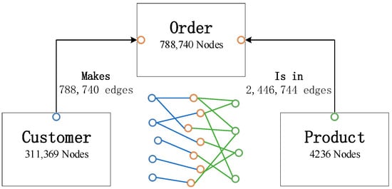
Figure 1.
Customer–order–product heterogenous graph.
Table 2.
Nodes, edges, and their attributes.
Our target is to predict whether there will be a return on an edge of Order–Product in an order. The challenge stems from the dynamic nature of the Customer–Order–Product heterogeneous graph, which evolves as new orders are generated over time. Our task involves predicting returns for new orders, rather than those already present in the graph during the training phase. Thus, our prediction approach is inductive rather than transductive.
Heterogeneous Graph Neural Networks (HGNNs) have emerged as a powerful tool for analyzing complex systems with diverse entities and relationships [25,26,27]. Unlike traditional Graph Neural Networks (GNNs) that operate on homogeneous graphs with uniform node and edge types, HGNNs excel in handling graphs with varying node and edge types. This flexibility enables them to model intricate relationships in real-world scenarios [28], such as social networks [29], text classification [30,31], recommendation systems [32,33], and biological networks [34], where entities can exhibit diverse characteristics and connections.
Our Customer–Order–Product Heterogeneous Graph Neural Networks (COP-HGNNs) for return prediction leverage three types of nodes and edges to capture nuanced information, enabling a deeper understanding of the underlying structures. By incorporating diverse node and edge types, our model is better equipped to discern intricate patterns. Our solution comprises two subnetworks: an inductive embedding network and a prediction network, both trained jointly in a supervised manner.
3.2.1. Inductive Embedding Network
We leverage node and edge features to learn an inductive embedding function that generalizes to unseen nodes and edges. Instead of training distinct embedding vectors for each node and edge, we train a set of embedding and aggregator functions that learn to aggregate feature information from neighboring nodes and edges. During inference, we apply these learned functions to generate embeddings for entirely unseen nodes, enabling predictions on new data.
Initially, we transform categorical variables such as customer ID, product ID, product group, color code, and size code into continuous representations through a feature embedding layer. Specifically, we use a fully connected linear layer that ensures each input index possesses an associated weight vector:
where is the one-hot vector representation of the nominal variable X. During the training process, the weight matrix is updated to learn the optimal embedding representations (C is the size of the dictionary of ; E is the size of each embedding vector).
Since the product node contains both numerical attributes (such as the recommended retail price listed in Table 2) and nominal attributes (such as Product Group), we utilize a linear layer to transform the dimension of the numerical attributes into E. The product node embedding is then a composite representation of the product ID embedding, the Product Group (a categorical feature of product) embedding, and the embedding of numerical attributes:
The edge embedding representation of the ‘order-product’ linkage is obtained by
where is the vector of numeric attributes, including ‘quantity’ and ‘discount’.
Generating the embedded representation of the order node involves capturing various facets, including details about the customer placing the order, the products contained within the order, and the distinct attributes of the order itself. We utilize the SAGE graph convolution with a mean aggregator [35] to aggregate the embedded representations of the products within the order into the order embedding:
where are network weight matrixes, and represents an indexing function that maps the order to the customer who placed it, utilizing the edge between the customer and the order.
3.2.2. Return Prediction Network
After obtaining the node and edge embedding representations, we use them as inputs to an MLP (Multilayer Perceptron) neural network to generate return prediction:
where and are weight matrices, [·] represents the concatenate operator, and converts x into the return probability.
3.2.3. Loss Function
The training of the COP-HGNN utilizes the Binary Cross-Entropy Loss function (BCE Loss) to evaluate prediction outcomes (as denoted in Equation (6)).
where y is either a 1 or 0, indicative of whether the product was returned or not, respectively. N signifies the overall number of training samples. We utilize the Adam optimization algorithm [36] to continuously update the network parameters via gradient back-propagation of the Loss function. This process assists in minimizing the discrepancy between the prediction results and the actual labels.
3.2.4. Online Prediction for New Orders
In the prediction stage, given the network weights obtained during training, we assume that when a customer places a new order, the prediction system can query the trained network to obtain the customer’s embedding representation via their Customer ID. We can similarly obtain the embedding vectors of each product in the order. The edge embedding can be calculated using Equation (3), and the order’s embedding representation can be calculated using Equation (4). Finally, the return probability prediction for each ordered product is calculated by applying Equation (5). In the event of new customers or new products (i.e., the ‘cold start problem’), the system will assign them a new ID code. During the network training phase, we have reserved ample embedding dimension space for these new customers or products.
The algorithm for the pseudo-training of both the embedding network and the return prediction network is outlined in Algorithm 1. Algorithm 2 encapsulates the predictive process for new orders.
| Algorithm 1: Training COP-HGNN embedding and return prediction network |
| Input: Nodes, node features, edges, and edge features. |
| Output: HGNN network with optimization weights. |
| 1 initializing network weights , |
| 2 for m in 1…MAX-STEPs do |
| 3 for batch in 1…MAX-NUM-BATCHs do |
| 4 for f in [customer, product, color, size, product group] do |
| # embedding customer, product, color, size, product group |
| 5 ; |
| 6 end |
| # embedding product |
| 7 ; |
| # embedding edge of order-product |
| 8 ; |
| # embedding order with graph convolution |
| 9 |
| # generating return prediction |
| 10 |
| 11 |
| end |
| 12 Backpropagate the network weights |
| 13 end |
| Algorithm 2: Return prediction for products in a new order |
| Input: embedding network, prediction network, Customer ID, IDs of products in the order, order features, order-product features. |
| Output: the return probability for each product in the order |
| 1 Calculating , , and using the COP-HGNN network weights; |
| 2 Calculating using graph convolution; |
| 3 for product in order do |
| 4 Generating return prediction using prediction network and embeddings; |
| 5 end |
4. Experiments
4.1. Experimental Setup
To train and test the return prediction networks, we initially partitioned the data into a test set and training set based on the timeline. The orders made in the first 21 months comprised the training set, while orders in the last 3 months formed the testing set for this study. The training set includes 2,293,521 transactional records, out of which 1,208,000 returns took place, accounting for 52.67%. The proportion of returns observed in the test set was consistent with that of the training set. Additionally, we further divided the training set into two datasets based on the timeline too, the training set and the validation set, at ratios of 70% and 30%, respectively. The validation set was utilized to optimize hyperparameters and the corresponding optimal training steps.
The vast number of nodes and edges within the graph make training on the entire graph model difficult due to computational limitations of GPU memory. As a result, we utilize the heterogeneous graph sampling algorithm introduced by [37] to segment and sample the complete graph to obtain a mini-batch. The heterogeneous graph sampling algorithm allocates a node budget for each node type, which determines the probability of node sampling. Specifically, the probability of sampling a node is determined considering the number of connections to already sampled nodes and their respective node degrees. Utilizing this method, the heterogeneous graph sampling algorithm selects a fixed quantity of neighbors for each node type in every iteration, denoted by the argument ‘number of samples’, which is set as 2048 in our experiments.
To optimize the proposed HGNN network, we select the embedding dimension E and learning rate ‘lr’ of the Adam optimizer as hyperparameters. The Adam optimization algorithm is preferred for optimizing graph neural networks due to its adaptive learning rate, memory efficiency, robustness to sparse gradients, and faster convergence speed. Due to the independence of these two hyperparameters, we employed a grid search approach to optimize them separately. The range of search space for embedding dimension E was set as [8, 12, 16, 24, and 32], while the learning rate’s search range was [0.1, 0.005, 0.001, and 0.0005]. We used the validation set to evaluate the hyperparameters and the corresponding optimal training steps were ultimately determined by an embedding vector dimension E of 12, learning rate of 0.001, and 25 training steps.
4.2. Baseline Models for Comparison
To assess the predictive accuracy of HGNN, we compared it with seven traditional machine learning classification algorithms as baseline models. These models include Logistic Regression, Naive Bayes, K-Nearest Neighbors, Classification and Regression Tree (CART), Random Forest, Gradient Boosting Decision Tree (GBDT), and LightGBM. Identically, for the COP-HGNN, we used all the features listed in Table 2 for training these models. Hyperparameters for all models were selected utilizing Bayesian optimization methods [38]. A brief introduction on those baseline models and the hyperparameters for training is listed below.
Logistic Regression (LR) is a fundamental statistical learning model employed to tackle classification challenges. By multiplying feature vectors with weights and adding bias terms, a linear function is obtained, which is then fed into the sigmoid function to obtain a probability output.
Naive Bayes (NB) is a basic classification algorithm grounded on Bayes’ theorem. It operates under the assumption that all features are independent of each other and have the same impact on the sample category. NB is simple, fast, easy to implement, and commonly used in fields such as text classification and spam filtering.
K-Nearest Neighbors (KNN) is a non-parametric classification method based on instance learning. It determines the category of test samples by calculating the distance between them and every sample in the training set. The advantages of KNN include simplicity, ease of implementation, and suitability for various classification issues. We employ Manhattan Distance to measure the distance between samples and optimize the number of nearest neighbors and the dimension of the Manhattan Distance as super parameters.
The Classification and Regression Tree (CART) is a probabilistic analysis model that classifies data by constructing a Binary tree. We select three super parameters for model optimization, including the maximum depth of the Binary tree (max depth), the minimum number of samples contained in the leaf node (min samples leaf), and the minimum number of samples required for node branching (min samples split).
Random Forests (RFs) employ bagging ensemble methods to enhance the predictive performance of a single decision tree [39]. We choose four hyperparameters to optimize the Random Forest classifier, including the number of decision trees (num of estimators), the maximum depth of each tree (max depth), the minimum number of samples for leaf nodes (min samples leaf), and the minimum number of samples required for node partitioning (min samples split).
Gradient Boosting Decision Tree (GBDT) is another ensemble learning algorithm and a method to enhance the model based on the decision tree. It gradually improves the model performance by fitting past prediction error residuals in each iteration. It was first proposed by [40]. There are three hyperparameters for GBDT tuning in this study: the maximum depth of each tree (max depth), the minimum number of samples required by internal nodes in partitioning (min samples split), and the learning rate (learning rate).
LightGBM is an efficient, fast, and distributed gradient elevation decision tree (GBDT) framework [41]. Compared with traditional GBDT algorithms, LightGBM adopts histogram-based decision tree learning algorithms and a leaf-wise growth strategy. Due to its efficient algorithm design and distributed computing capabilities, LightGBM has been extensively used in tasks such as the classification, regression, and sorting of large-scale datasets and has achieved significant results in multiple data mining competitions. We opt to tune two hyperparameters of LightGBM, including the maximum depth (max depth) and learning rate (learning rate).
4.3. Evaluation Metrics
We utilize five metrics to evaluate the prediction accuracy of the COP-HGNN and its benchmarks: Accuracy, Precision, Recall, F1-Score, and area under the Receiver Operating Characteristic curve (AUC).
4.4. Results
In Table 3, we evaluate the accuracy of each prediction model for all orders in the test set using a return probability of 0.5 as the threshold to determine whether a product will be returned upon purchase. The LightGBM model had the best performance with an AUC value of 0.7099 and the highest Accuracy, Precision, and F1-Score values. The COP-HGNN followed closely in second place with an AUC value of 0.6864 and similar results to LightGBM for other evaluation indicators. The GBDT performed average compared to the COP-HGNN.
Table 3.
Overall comparison results across the entire test sample.
In Table 4, we further evaluate the accuracy of each model for orders made by repeat customers in the test set. Repeat customers here refer to those who appeared in the training sets that made at least one purchase, while new customers denote those who made their first purchase during the periods of the test set. In the test set, there are 73,030 unique customer IDs. Among them, 42,361 are repeat customers and 30,669 are new customers. Among repeat customers, 23,459 had purchased more than three times in the training set, and 14,874 customers had purchased more than five times.
Table 4.
Comparison results on returns by repeat customers.
Table 4 reveals that the COP-HGNN model had significant advantages in predicting returns from repeat customers. The COP-HGNN achieved an AUC of 0.7122, which was 3.2 percentage points higher than the sample containing new customers. Additionally, its Accuracy and Precision were also highest, with increases of 2.25 and 3.74 percentage points, respectively. However, traditional machine learning models’ prediction accuracy remained largely unchanged with only a marginal increase in AUC for the LightGBM model and a slight decrease for GBDT and RF models. Therefore, the results suggest that the COP-HGNN is more suitable for predicting returns for repeat customers, while predicting returns from new customers remains challenging.
Table 5 and Table 6 provide a further analysis of each model’s performance in predicting returns for customers who made three or more purchases in the training set. As the number of purchases increased, the COP-HGNN’s prediction accuracy improved further. For instance, when customers made more than three purchases in the training set, the AUC of the HGNN model was 0.7287, while it reached 0.7311 when customers made more than five purchases. In contrast, except for the slight increase in the prediction accuracy of Logistic Regression and LightGBM, the remaining machine learning models continued to decline as customers’ purchase times increased.
Table 5.
Return prediction performance comparisons for customers with three or more purchases in the training set.
Table 6.
Return prediction performance comparisons for customers with five or more purchases in the training set.
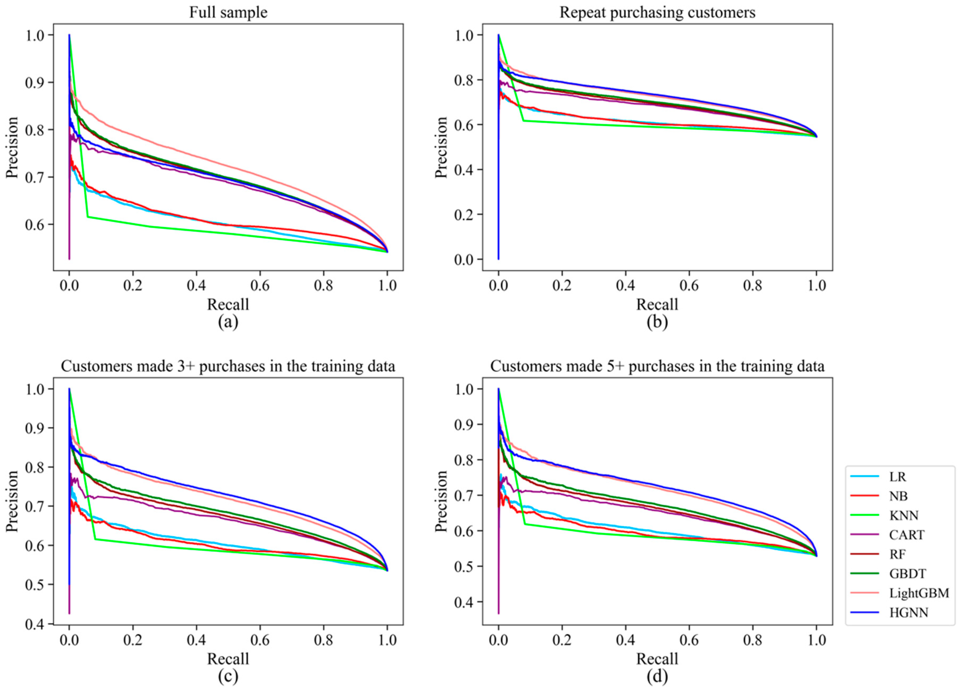
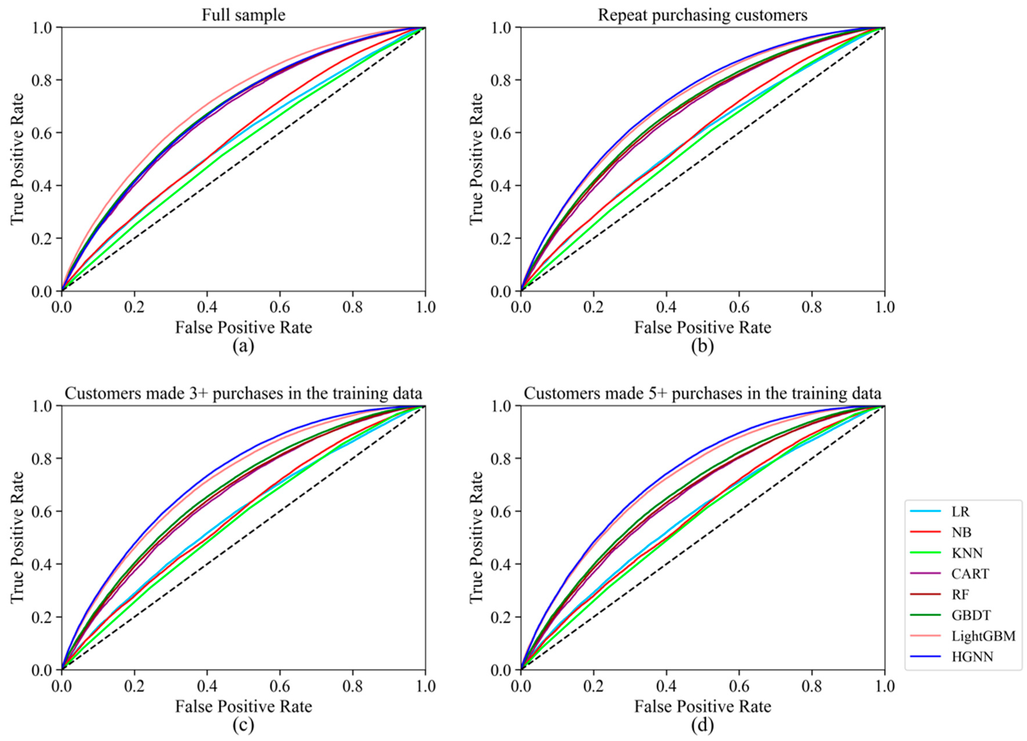
However, although the COP-HGNN performed excellently in Accuracy, Precision, and F1-Score indicators except for AUC, as shown in Table 4, Table 5 and Table 6, all the results are based on a 0.5 threshold to determine whether a product will be returned. To further test the return forecast performance of the COP-HGNN, we draw Precision–Recall curves and Receiver Operating Characteristic (ROC) curves in Figure 2 and Figure 3, respectively. The Precision–Recall curve in Figure 2a targets all customers in the test set, while those in Figure 2b–d target only repeat customers who made purchases one, three, and five times in the training set, respectively, corresponding to Table 4, Table 5 and Table 6. It can be observed that for repeat customers, the COP-HGNN model maintained the highest prediction accuracy under the same Recall score.
Figure 2.
Precision–Recall curve. (a) Full data sample with all customers; (b) data sample with only repeat customers; (c) data sample with repeat customers who made purchase at least three times in the training data; (d) data sample with repeat customers who made purchase at least five times in the training data.

Figure 3.
Receiver Operating Characteristic curve. (a) Full data sample with all customers; (b) data sample with only repeat customers; (c) data sample with repeat customers who made purchase at least three times in the training data; (d) data sample with repeat customers who made purchase at least five times in the training data.
Moreover, as shown in the ROC curves in Figure 3, the COP-HGNN had the lowest False Positive Rate for repeat customers under the same True Positive Rate. Therefore, these results suggest that the COP-HGNN model might be a better fit for identifying the potential returning customers for businesses with a focus on customer retention.
4.5. Ablation Analysis
To assess the significance of customer, order, and product embeddings in predicting product returns, we conducted additional experiments using two HGNN models as benchmarks. The first model, termed OP-HGNN, omits the customer embedding described as the second component in Equation (4). Meanwhile, the second benchmark, CP-HGNN, excludes both order attributes (the first component in Equation (4)) and information pertaining to products within the order (the third component in Equation (4)).
The AUC comparisons presented in Table 7 reveal the significance of different embedding components within COP-HGNNs for predicting product returns. It is evident that both customer and order embeddings play crucial roles in this prediction task. Notably, OP-HGNN demonstrates limited effectiveness in predicting product returns for repeat customers. While CP-HGNN shows improvement in this aspect compared to OP-HGNN, it still falls short when compared to the COP-HGNN.
Table 7.
AUC comparisons of HGNNs with different embedding components.
5. Conclusions
By predicting customers’ return behavior, online fast fashion retailers can provide early warning signals and take timely intervention measures to reduce the possibility of return in advance. This would lead to cost reductions and improved operational efficiency. In this study, we propose a proactive return prediction model based on the Heterogeneous Graph Neural Network to address high return rates among online fast fashion retailers. The model establishes customers, orders, and products as nodes, with indirect connections established between customers and products through orders. By training neural networks, hidden feature vectors can be constructed for customers, orders, and products, enabling the prediction of customer return behavior for a specific product in a new order. This approach allows each node of the graph to embed into a feature vector and utilize edges with features to transmit information in the graph, capturing a comprehensive graph structure.
The empirical results demonstrate that the proposed COP-HGNN model performs better than the baseline models in predicting returns for repeat purchase customers. Moreover, prediction accuracy improves as the number of repeat purchases increases. However, the COP-HGNN’s return prediction ability for new customers remains insufficient. This suggests that customer characteristics are critical to predicting their return behavior, and the COP-HGNN can construct implicit features based on customer historical order information. Conversely, for new customers with limited preference information, the randomly constructed implicit features consequently weaken the HGNN model’s return prediction ability. The ablation analyses underscored the critical importance of concurrently considering the characteristics of customers, orders, and products in a proactive return prediction model.
Among all baseline models, the LightGBM model performs significantly better in return forecasting, especially for new customers. Given the complementarity between LightGBM and HGNN, online fast fashion retailers can utilize the LightGBM model to predict the return behavior of new customers and leverage the COP-HGNN to predict the return behavior of repeat purchase customers.
In addition to highlighting the strengths of our graph neural network model in proactively predicting product returns, it is essential to acknowledge its limitations. One significant limitation pertains to the potential biases inherent in the dataset used for training and evaluation. Despite efforts to ensure data quality and integrity, biases such as sampling bias or selection bias may still exist, potentially influencing the model’s predictions. Additionally, the performance of our model may vary under different market conditions or contexts not fully captured by the dataset. Factors such as changes in consumer preferences, economic fluctuations, or unforeseen external events could impact the predictive accuracy of the model. Moreover, the effectiveness of proactive prediction strategies may be influenced by the dynamic nature of markets and evolving customer behaviors, warranting further exploration and adaptation of the model over time. Recognizing these limitations is essential for interpreting the model’s predictions accurately and for guiding future research efforts aimed at enhancing the robustness and generalizability of predictive models in real-world scenarios.
Future research endeavors could concentrate on refining the network architecture of the COP-HGNN, devising tailored information transmission mechanisms among nodes, and conducting thorough empirical and applied investigations to assess the model’s efficacy across diverse datasets and market scenarios. Additionally, enhancing the computational efficiency and scalability of Heterogeneous Graph Neural Networks for large-scale graph data could be a focal point, achieved through exploring optimization algorithms leveraging graph structure, distributed computing strategies, and accelerated hardware techniques.
Author Contributions
Conceptualization, S.M.; methodology, S.M.; software, S.M.; validation, W.W.; formal analysis, S.M.; data curation, S.M. and W.W.; writing—original draft preparation, W.W.; writing—review and editing, S.M.; visualization, W.W.; supervision, S.M.; project administration, S.M.; funding acquisition, S.M. All authors have read and agreed to the published version of the manuscript.
Funding
This research was funded by the National Natural Science Foundation of China, grant number 72072092.
Data Availability Statement
We have made our code and data for implementing the COP-HGNN available on github.com/Shawn-nau/HGNN.
Conflicts of Interest
The authors declare no conflicts of interest.
Abbreviations
| Adam | Adaptive Moment Estimation |
| AUC | Area Under the Curve |
| BPR | Bayesian Personalized Ranking |
| CART | Classification and Regression Tree |
| COP-HGNN | Customer–Order–Product Heterogeneous Graph Neural Network |
| KNN | K-Nearest Neighbors |
| LASSO | Least Absolute Shrinkage and Selection Operator |
| LightGBM | Light Gradient Boosting Machine |
| LR | Logistic Regression |
| GBDT | Gradient Boosting Decision Tree |
| NB | Naive Bayes |
| RF | Random Forests |
| ROC | Receiver Operating Characteristic curve |
| SAGE | SAmple and aggreGatE |
References
- Urbanke, P.; Kranz, J.; Kolbe, L.M. Predicting Product Returns in E-Commerce: The Contribution of Mahalanobis Feature Extraction. In Proceedings of the International Conference on Interaction Sciences, Fort Worth, TX, USA, 13–16 December 2015. [Google Scholar]
- Edwards, J.B.; McKinnon, A.C.; Cullinane, S.L. Comparative analysis of the carbon footprints of conventional and online retailing. Int. J. Phys. Distrib. Logist. Manag. 2010, 40, 103–123. [Google Scholar] [CrossRef]
- Duong, Q.H.; Zhou, L.; Meng, M.; Nguyen, T.V.; Ieromonachou, P.; Nguyen, D.T. Understanding product returns: A systematic literature review using machine learning and bibliometric analysis. Int. J. Prod. Econ. 2022, 243, 108340. [Google Scholar] [CrossRef]
- Ambilkar, P.; Dohale, V.; Gunasekaran, A.; Bilolikar, V. Product returns management: A comprehensive review and future research agenda. Int. J. Prod. Res. 2022, 60, 3920–3944. [Google Scholar] [CrossRef]
- Pei, Z.; Paswan, A. Consumers’ legitimate and opportunistic product return behaviors in online shopping. J. Electron. Commer. Res. 2018, 19, 301–319. [Google Scholar]
- Wen, X.; Choi, T.-M.; Chung, S.-H. Fashion retail supply chain management: A review of operational models. Int. J. Prod. Econ. 2019, 207, 34–55. [Google Scholar] [CrossRef]
- Abdulla, H.; Ketzenberg, M.; Abbey, J.D. Taking stock of consumer returns: A review and classification of the literature. J. Oper. Manag. 2019, 65, 560–605. [Google Scholar] [CrossRef]
- Li, X.; Ma, B.; Chu, H. The impact of online reviews on product returns. Asia Pac. J. Mark. Logist. 2021, 33, 1814–1828. [Google Scholar] [CrossRef]
- Lv, J.; Liu, X. The Impact of Information Overload of E-Commerce Platform on Consumer Return Intention: Considering the Moderating Role of Perceived Environmental Effectiveness. Int. J. Environ. Res. Public Health 2022, 19, 8060. [Google Scholar] [CrossRef]
- Chang, H.-H.; Guo, Y.-Y. Online fraudulent returns in Taiwan: The impacts of e-retailers’ transaction ethics and consumer personality. J. Retail. Consum. Serv. 2021, 61, 102529. [Google Scholar] [CrossRef]
- Serravalle, F.; Vannucci, V.; Pantano, E. “Take it or leave it?”: Evidence on cultural differences affecting return behaviour for Gen Z. J. Retail. Consum. Serv. 2022, 66, 102942. [Google Scholar] [CrossRef]
- Bechwati, N.N.; Siegal, W.S. The Impact of the Prechoice Process on Product Returns. J. Mark. Res. 2005, 42, 358–367. [Google Scholar] [CrossRef]
- Shehu, E.; Papies, D.; Neslin, S.A. Free Shipping Promotions and Product Returns. J. Mark. Res. 2020, 57, 640–658. [Google Scholar] [CrossRef]
- Rao, S.; Rabinovich, E.; Raju, D. The role of physical distribution services as determinants of product returns in Internet retailing. J. Oper. Manag. 2014, 32, 295–312. [Google Scholar] [CrossRef]
- Hjort, K.; Lantz, B. The impact of returns policies on profitability: A fashion e-commerce case. J. Bus. Res. 2016, 69, 4980–4985. [Google Scholar] [CrossRef]
- Janakiraman, N.; Syrdal, H.A.; Freling, R. The Effect of Return Policy Leniency on Consumer Purchase and Return Decisions: A Meta-analytic Review. J. Retail. 2016, 92, 226–235. [Google Scholar] [CrossRef]
- Bahn, K.D.; Boyd, E. Information and its impact on consumers’ reactions to restrictive return policies. J. Retail. Consum. Serv. 2014, 21, 415–423. [Google Scholar] [CrossRef]
- Dzyabura, D.; El Kihal, S.; Hauser, J.R.; Ibragimov, M. Leveraging the Power of Images in Managing Product Return Rates. Mark. Sci. 2019, 42, 1125–1142. [Google Scholar] [CrossRef]
- Cui, H.; Rajagopalan, S.; Ward, A.R. Predicting product return volume using machine learning methods. Eur. J. Oper. Res. 2020, 281, 612–627. [Google Scholar] [CrossRef]
- Rajasekaran, V.; Priyadarshini, R. An E-Commerce Prototype for Predicting the Product Return Phenomenon Using Optimization and Regression Techniques; Springer International Publishing: Cham, Switzerland, 2021; pp. 230–240. [Google Scholar]
- Tuylu, A.N.A.; Eroğlu, E. The prediction of product return rates with ensemble machine learning algorithms. J. Eng. Res. 2022. [Google Scholar] [CrossRef]
- Zhu, Y.; Li, J.; He, J.; Quanz, B.; Deshpande, A.A. A Local Algorithm for Product Return Prediction in E-Commerce. In Proceedings of the International Joint Conference on Artificial Intelligence, Stockholm, Sweden, 13–19 July 2018. [Google Scholar]
- Li, J.; He, J.; Zhu, Y. E-tail Product Return Prediction via Hypergraph-based Local Graph Cut. In Proceedings of the 24th ACM SIGKDD International Conference on Knowledge Discovery & Data Mining, London, UK, 19–23 August 2018; Association for Computing Machinery: New York, NY, USA, 2018; pp. 519–527. [Google Scholar]
- Kedia, S.; Madan, M.; Borar, S. Early Bird Catches the Worm: Predicting Returns Even Before Purchase in Fashion E-commerce. arXiv 2019, arXiv:1906.12128. [Google Scholar]
- Zhang, C.; Song, D.; Huang, C.; Swami, A.; Chawla, N.V. Heterogeneous Graph Neural Network. In Proceedings of the 25th ACM SIGKDD International Conference on Knowledge Discovery & Data Mining, Anchorage, AK, USA, 4–8 August 2019; Association for Computing Machinery: New York, NY, USA, 2019; pp. 793–803. [Google Scholar]
- Long, Q.; Xu, L.; Fang, Z.; Song, G. HGK-GNN: Heterogeneous Graph Kernel based Graph Neural Networks. In Proceedings of the 27th ACM SIGKDD Conference on Knowledge Discovery & Data Mining, Virtual Event, Singapore, 14–18 August 2021; Association for Computing Machinery: New York, NY, USA, 2021. [Google Scholar]
- Jia, X.; Jiang, M.; Dong, Y.; Zhu, F.; Lin, H.; Xin, Y.; Chen, H. Multimodal heterogeneous graph attention network. Neural Comput. Appl. 2023, 35, 3357–3372. [Google Scholar] [CrossRef]
- Bing, R.; Yuan, G.; Zhu, M.; Meng, F.; Ma, H.; Qiao, S. Heterogeneous graph neural networks analysis: A survey of techniques, evaluations and applications. Artif. Intell. Rev. 2023, 56, 8003–8042. [Google Scholar] [CrossRef]
- Salamat, A.; Luo, X.; Jafari, A. HeteroGraphRec: A heterogeneous graph-based neural networks for social recommendations. Knowl. Based Syst. 2021, 217, 106817. [Google Scholar] [CrossRef]
- Chen, Z.; Ji, W.; Ding, L.; Song, B. Document-level multi-task learning approach based on coreference-aware dynamic heterogeneous graph network for event extraction. Neural Comput. Appl. 2023, 36, 303–321. [Google Scholar] [CrossRef]
- Li, H.; Yan, Y.; Wang, S.; Liu, J.; Cui, Y. Text classification on heterogeneous information network via enhanced GCN and knowledge. Neural Comput. Appl. 2023, 35, 14911–14927. [Google Scholar] [CrossRef]
- Afoudi, Y.; Lazaar, M.; Hmaidi, S. An enhanced recommender system based on heterogeneous graph link prediction. Eng. Appl. Artif. Intell. 2023, 124, 106553. [Google Scholar] [CrossRef]
- Do, P.; Pham, P. Heterogeneous graph convolutional network pre-training as side information for improving recommendation. Neural Comput. Appl. 2022, 34, 15945–15961. [Google Scholar] [CrossRef]
- Ma, A.; Wang, X.; Li, J.; Wang, C.; Xiao, T.; Liu, Y.; Cheng, H.; Wang, J.; Li, Y.; Chang, Y.; et al. Single-cell biological network inference using a heterogeneous graph transformer. Nat. Commun. 2023, 14, 964. [Google Scholar] [CrossRef]
- Hamilton, W.L.; Ying, R.; Leskovec, J. Inductive representation learning on large graphs. In Proceedings of the 31st International Conference on Neural Information Processing Systems, Long Beach, CA, USA, 4–9 December 2017; Curran Associates Inc.: Red Hook, NY, USA, 2017; pp. 1025–1035. [Google Scholar]
- Kingma, D.P.; Ba, J. Adam: A Method for Stochastic Optimization. In Proceedings of the 3rd International Conference for Learning Representations, San Diego, CA, USA, 7–9 May 2015. [Google Scholar]
- Hu, Z.; Dong, Y.; Wang, K.; Sun, Y. Heterogeneous Graph Transformer. In Proceedings of the Web Conference 2020, Taipei, Taiwan, 20–24 April 2020; Association for Computing Machinery: New York, NY, USA, 2020; pp. 2704–2710. [Google Scholar]
- Frazier, P. A Tutorial on Bayesian Optimization. arXiv 2018, arXiv:1807.02811. [Google Scholar]
- Breiman, L. Random Forests. Mach. Learn. 2001, 45, 5–32. [Google Scholar] [CrossRef]
- Friedman, J.H. Greedy function approximation: A gradient boosting machine. Ann. Stat. 2001, 29, 1189–1232. [Google Scholar] [CrossRef]
- Ke, G.; Meng, Q.; Finley, T.; Wang, T.; Chen, W.; Ma, W.; Ye, Q.; Liu, T.-Y. LightGBM: A highly efficient gradient boosting decision tree. In Proceedings of the 31st International Conference on Neural Information Processing Systems, Long Beach, CA, USA, 4–9 December 2017; Curran Associates Inc.: Red Hook, NY, USA, 2017; pp. 3149–3157. [Google Scholar]
Disclaimer/Publisher’s Note: The statements, opinions and data contained in all publications are solely those of the individual author(s) and contributor(s) and not of MDPI and/or the editor(s). MDPI and/or the editor(s) disclaim responsibility for any injury to people or property resulting from any ideas, methods, instructions or products referred to in the content. |
© 2024 by the authors. Licensee MDPI, Basel, Switzerland. This article is an open access article distributed under the terms and conditions of the Creative Commons Attribution (CC BY) license (https://creativecommons.org/licenses/by/4.0/).