Renal Pathological Image Classification Based on Contrastive and Transfer Learning

Abstract

Following recent advancements in medical laboratory technology, the analysis of high-resolution renal pathological images has become increasingly important in the diagnosis and prognosis prediction of chronic nephritis. In particular, deep learning has been widely applied to computer-aided diagnosis, with an increasing number of models being used for the analysis of renal pathological images. The diversity of renal pathological images and the imbalance between data acquisition and annotation have placed a significant burden on pathologists trying to perform reliable and timely analysis. Transfer learning based on contrastive pretraining is emerging as a viable solution to this dilemma. By incorporating unlabeled positive pretraining images and a small number of labeled target images, a transfer learning model is proposed for high-accuracy renal pathological image classification tasks. The pretraining dataset used in this study includes 5000 mouse kidney pathological images from the Open TG-GATEs pathological image dataset (produced by the Toxicogenomics Informatics Project of the National Institutes of Biomedical Innovation, Health, and Nutrition in Japan). The transfer training dataset comprises 313 human immunoglobulin A (IgA) chronic nephritis images collected at Fukushima Medical University Hospital. The self-supervised contrastive learning algorithm “Bootstrap Your Own Latent” was adopted for pretraining a residual-network (ResNet)-50 backbone network to extract glomerulus feature expressions from the mouse kidney pathological images. The self-supervised pretrained weights were then used for transfer training on the labeled images of human IgA chronic nephritis pathology, culminating in a binary classification model for supervised learning. In four cross-validation experiments, the proposed model achieved an average classification accuracy of 92.2%, surpassing the 86.8% accuracy of the original RenNet-50 model. In conclusion, this approach successfully applied transfer learning through mouse renal pathological images to achieve high classification performance with human IgA renal pathological images.

1. Introduction

1.1. Chronic Nephritis Diagnosis

Chronic nephritis is an inflammation of the glomerulus that can affect urinary function and cause body swelling. It is often caused by infections and toxins but is most commonly caused by autoimmune diseases. Human immunoglobulin A (IgA) nephritis is the most common condition worldwide and is associated with human immune responses [1]. When IgA is released and remains in kidneys, inflammation can occur [2]. Although IgA nephritis does not cause significant symptoms in its early stages, the inflammation causes leakage of blood and proteins. The kidney gradually loses its functionality, eventually leading to kidney failure [3].

For patients with IgA nephritis, it is important to diagnose and identify the stage of the nephritis. Pathologists often perform kidney biopsies to diagnose suspected kidney disease. This is performed by inserting a thin needle through the skin to obtain kidney tissue under ultrasound or imaging-device localization [4]. The kidney tissue is finely sliced, and histological changes are observed under an optical microscope [5]. This provides valuable information for the diagnosis of kidney disease.

High-resolution optical microscopes manufactured by leading companies such as Leica and Olympus [6] are capable of scanning sections of kidney tissue and digitally storing them as whole-slide images (WSIs) [7]. This technological advancement has greatly facilitated diagnostic and research processes associated with chronic nephritis. WSIs with high resolution and large image sizes provide comprehensive and detailed views of tissue samples [8]. However, IgA nephritis has a high prevalence in East Asia. The global incidence of IgA nephritis is 2.5 per 100,000 adults per year, and the task of analyzing these renal pathological images represents a significant workload for pathologists [9]. A typical analysis of a renal biopsy specimen can take several days [10]. Given these challenges, implementing a computer-aided diagnostic system represents a major step toward improved analysis efficiency and timely diagnosis.

1.2. Progress and Weaknesses of Supervised Learning in Renal Pathological Image Analysis

The key to renal pathological image analysis is the identification of glomerulus. In recent years, supervised learning models have been applied to this task [11]. Various studies have considered the application of deep learning to renal pathology, particularly for the analysis of complex histological structures within the kidney.

For the detection and classification of glomerulus, Gallego et al. proposed a Convolutional Neural Network (CNN) that utilizes a pretrained AlexNet model. They adapted this model for the classification of glomerulus by training it to learn from the glomerulus and non-glomerulus regions extracted from the training slides [12]. Uchino et al. implemented a classification model by fine-tuning their InceptionV3 model for seven types of glomerulus morphological changes [13]. Chagas et al. introduced a method that incorporates a novel architecture of a CNN in conjunction with a Support Vector Machine. This method achieved near-perfect average results on the FIOCRUZ dataset in the binary classification of glomerulus [14].

For glomerulus segmentation tasks, Dimitri et al. utilized the DeepLab V2 model, which was pretrained with a Residual Network (ResNet)-101 encoder. They applied this model to 512 × 512 pixel patches that were extracted from the original WSIs for segmentation, despite the variations in coloring and typology in the pathological images [15]. Gu et al. introduced a multistream framework built upon three prominent models (FCN, Deeplabv3, and UNet) for glomerulus segmentation [16].

These algorithms have demonstrated their ability to process images with a high accuracy, even approaching the accuracy of pathologists. This highlights the ability of deep learning to improve the efficiency and accuracy of renal pathological image analysis. However, there remain limitations to these approaches. Whether it is image-level annotations for classification, bounding boxes for detection, or pixel-level annotations for segmentation, each task heavily relies on the expertise of pathologists. As the training set continues to grow, pathologists will be overwhelmed by the sheer volume of data to annotate.

1.3. Motivation

The concepts of contrastive learning and transfer learning can provide potential solutions to these challenges. Contrastive learning is a self-supervised learning strategy that is based on the principle of bringing similar “positive” samples closer together in an embedding space while distancing “negative” samples. This approach enables the effective use of large amounts of unlabeled data and significantly reduces pathologists’ workload. Transfer learning is a technique for reusing a model once it has been trained on a particular task by taking the model weights as the starting point for another related task [17]. This method promotes efficiency and accelerates the learning process.

In recent years, applications of contrastive learning and transfer learning have been implemented for classification tasks in various domains. Wang et al. developed a semi-supervised learning framework for Mars imagery classification based on contrastive learning, demonstrating the applicability of contrastive methods in improving classification accuracy in planetary exploration scenarios [18]. Kato et al. utilized contrastive learning for COVID-19 pneumonia classification from CT images, highlighting the efficacy of contrastive learning methods in training new classifiers following initial steps [19]. Wu and Lin investigated the impact of transfer learning on the performance of VGGNet-16 and ResNet-50 for classifying organic and residual waste [20]. Their study highlighted the benefits of deep learning with transfer learning in waste classification tasks, showcasing its potential in environmental applications. Alzubaidi et al. introduced a novel transfer learning approach for medical imaging tasks with limited labeled data [21]. By combining transfer learning with contrastive pretraining, the performance of convolutional neural networks was enhanced in medical image classification. Overall, the implementation of contrastive learning and transfer learning techniques offers promising avenues for classification tasks, enabling models to learn robust representations and generalize well across different domains and datasets.

In this research, we propose a WSI classification model for human IgA nephritis that is based on contrastive pretraining, with the aim of reducing the burden on pathologists. We also aimed to improve the performance of the model using the transfer learning approach. ResNet [22] was selected as the backbone of the classification model, and mouse glomerulus images were used in the contrastive pretraining process. The “Bootstrap Your Own Latent” (BYOL)-based contrastive learning algorithm [23] was used to extract feature representations of mouse glomerulus images. In the transfer learning phase, a small number of labeled human nephritis WSIs were used to train a binary classification model. This model could classify kidney pathology images from glomerulus images and other images, and it outperformed a supervised learning model based on the same backbone.

2. Materials and Methods

2.1. Materials

The original mouse kidney images used in this study were provided freely by the Toxicogenomics Informatics Project of the National Institutes of Biomedical Innovation, Health, and Nutrition (NIBIOHN) in Japan [24]. The original human kidney images were provided by Fukushima Medical University Hospital. This research was approved by the Institutional Review Board of Fukushima Medical University and was performed based on the Declaration of Helsinki.

2.1.1. Mouse Glomerulus Images for Contrastive Pretraining

The mouse glomerulus image dataset comprised high-resolution WSIs of pathological kidney specimens stained with hematoxylin-eosin dyes [24]. The specimens were obtained from animal experiments. The digitization of these images was performed with the virtual sliding Leica Aperio Scan Scope, ID number SS1061, Leica Corp., Wetzlar, Germany [24]. The images were digitized at a maximum magnification of 20× and a spatial resolution of 0.5 microns per pixel (mpp) [24]. The original pathological images were processed and selected to give 5000 image patches with glomerulus at a size of 256 × 256. Figure 1 shows the original WSI of a mouse kidney affected by 1% cholesterol and 0.25% sodium cholate.

To avoid the morphology of the glomerulus of mouse under different regimens affecting the results, equal-sized sets of images for two different drug regimens affecting inputs were selected. The dataset formed by images affected by 1% cholesterol and 0.25% sodium cholate was called mouse dataset A. The dataset formed by images affected by nitrofluorene was called mouse dataset B.

2.1.2. IgA Glomerulus Images for Contrastive Pretraining and Transfer Learning

The IgA glomerulus image dataset comprised periodic-acid-Schiff–stained human pathological images from 313 chronic kidney disease cases treated at Fukushima Medical University Hospital between 2002 and 2018. The digitization of these images was performed with the virtual sliding Leica Aperio Scan Scope, ID number SS7572, Leica Corp., Wetzlar, Germany. The images were digitized at a maximum magnification of 40× and a spatial resolution of 0.25 mmp. The original pathological images were subsequently cropped into patches of 256 × 256 pixels at a magnification of 8×, which corresponds to a spatial resolution of 1.25 mpp. This process resulted in a dataset comprising image patches, inclusive of 7000 glomerulus-containing and 7000 non-glomerulus-containing images. The dataset was then partitioned into training, validation, and test sets in a 7:1:2 ratio. Each set contained images from distinct cases. Figure 2 shows the original WSI from a patient with IgA nephritis.

Concerning the learning performance of the model, each image in the dataset was carefully categorized by pathologists to ensure the accuracy of the training data. Figure 3 shows image patches containing human and mouse glomerulus processed from the original WSIs. The left and right images are from a patient with IgA and a mouse, respectively.

2.2. Classification Backbone ResNet

ResNet (Residual Network), a deep learning architecture proposed in 2015, has become a reliable choice for a wide range of classification tasks. ResNet has demonstrated competitive performance and robustness in various tasks of medical image analysis, such as glaucoma detection [25], bone lesion staging [26], and cervical cancer diagnosis [27]. Furthermore, the structure of ResNet is relatively simple and intuitive, facilitating adjustment and reproduction. The choice of the ResNet backbone helps to improve the interpretability of the results.

The defining characteristic of ResNet is the use of residual blocks. As given in Equation (1), the residual blocks allow the network to learn the residual mapping between inputs and outputs, where x is the input, $F\left(x\right)$ is the feature mapping processed by convolutional layers, and $G\left(x\right)$ is the output mapping. The problems of gradient vanishing and gradient explosion can be mitigated with this design, allowing the integration of additional convolutional layers [22].

$$G\left(x\right)=F\left(x\right)+x$$

(1)

The residual block consists of two main paths: the convolutional path and the shortcut path. As shown in Figure 4, where the number of input and output channels is the same, the structure of the residual block involves the convolutional path applying a series of convolutional layers followed by batch normalization (BN) and activation functions, such as ReLU. In this scenario, the shortcut path involves identity mapping, where the input is directly added to the output of the convolutional path [28]. The residual block is called an identity block in this situation.

As shown in Figure 5, when the number of input and output channels differs, the shortcut path needs to adjust the dimensions of the input to match the output dimensions before adding it to the output of the convolutional path. The adjustment is achieved by introducing an additional convolutional layer in the shortcut path. This convolutional layer changes the number of channels of the input tensor to align with the output tensor, ensuring that they can be element-wise added together [28]. The residual block is called a convolutional block in this situation.

The final feature mapping extracted by the ResNet backbone serves as a high-level abstract representation of the input data, capturing important features relevant to the subsequent classification task. This feature representation is then processed in a fully connected layer and Softmax for classification [29].

2.3. Contrastive Learning Method BYOL

BYOL is an innovative approach to self-supervised learning that aims to learn a representation that applies to downstream tasks [23]. As shown in Figure 6, the core concept of BYOL involves the use of two structurally similar neural networks, an online network, and a target network. The two neural networks have the same backbone and are trained to predict representations of the same image under different augmentations [23]. The online network also generates a prediction of the target network’s projection based on the obtained projection. The online network’s prediction is compared to the target network projection, and the difference is calculated as the training loss [23].

In this study, BYOL was employed to obtain the feature representations for images with glomerulus. BYOL has several advantages that fit with the medical image analysis model:

• Robustness to image augmentation: BYOL learns representations by comparing augmented pairs of the input. The model is trained to learn augmented invariant features, enhancing the ability to capture more representative features [30]. This helps to combat variability in medical images, such as slice fading.
• No reliance on negative pairs: BYOL does not rely on negative pairs in its training objective [23]. It establishes an invisible relationship between positive features through image enhancement, facilitating the full use of positive data.
• Performance improvement: BYOL has demonstrated superior performance [31] and robustness to batch size variations [32] on ImageNet compared to several contrastive learning methods, including SimCLR and MoCo.

2.4. Experimental Design

2.4.1. Optimizer and Loss Functions

The optimization strategy used in this study was stochastic gradient descent (SGD), which is an iterative method with an appropriate level of smoothness. SGD introduces randomness into the optimization process using a random subset of the entire dataset (a batch) to compute the gradient at each step, rather than the entire dataset [33]. This randomness can help avoid shallow local minima, making SGD more suitable for the non-convex error surfaces that are common in neural networks [34]. The SGD update rule is given in Equation (2), where ${\theta }_t$ is the parameter vector at iteration t and $\gamma$ is the learning rate. $\nabla f\left({\theta }_{t-1}\right)$ is the gradient of the loss function f with respect to the parameters at iteration $t-1$.

$${\theta }_t={\theta }_{t-1}-\gamma \nabla f\left({\theta }_{t-1}\right)$$

(2)

In the contrastive learning phase, layer-wise adaptive rate scaling (LARS) based on SGD was applied. LARS is an optimization algorithm used in deep learning to adjust the learning rate of each parameter based on its recent gradients [35]. In LARS, a different learning rate is introduced for each layer to ensure stable updates regardless of the difference in the ratio of the norm of the parameter to the norm of the gradient [36]. The learning rate for the parameter of each layer is determined at the time of parameter update, as given in Equation (3), where ${\lambda }_l$ is the learning rate for the parameter of layer l, $\eta$ is the confidence hyperparameter, $w_l$ is the parameter of layer l, and $\nabla L\left(w_l\right)$ is the gradient of the loss function with respect to the parameter of layer l.

$${\lambda }_l=\eta \times \frac{\parallel w_l\parallel }{\parallel \nabla L\left(w_l\right)\parallel }$$

(3)

In the contrastive pretraining phase, the loss function is determined by BYOL. BYOL employs a loss function that approximates cosine similarity, encouraging the online and target networks to generate similar image representations. The cosine similarity, $S_C(A,B)$, is defined by Equation (4) [37]. The parameters of the target network are gradually adjusted according to the updates of the parameters of the online network during training. The original definition of the BYOL loss functions is illustrated by Equation (5). As shown in Figure 6 and Equation (6), v and $v^{\prime }$ are images augmented from the same input x. $y_{\theta }$ and $y_{\xi }^{\prime }$ are the feature representations of v and $v^{\prime }$ generated by the online network $f_{\theta }$ and the target network $f_{\xi }$, respectively. $z_{\theta }$ and $z_{\xi }^{\prime }$ correspond to the projections of $y_{\theta }$ and $y_{\xi }^{\prime }$, respectively. $z_{\theta }$ is used to output the projection $q_{\theta }\left(z_{\theta }\right)$ in the online network. The ${\tilde{\mathcal{L}}}_{\theta ,\xi }$ is generated by processing $v^{\prime }$ with the online network and v with the target network reversely [23]. The value range of the BYOL loss function is often adjusted to be similar to that of the cosine function for better evaluation [38]. In our study, the value range of ${\mathcal{L}}_{\theta ,\xi }^{\mathrm{BYOL}}$ was adjusted to [$-4$,4]. The closer the loss value approaches $-4$, the smaller the difference between the feature vectors.

$$cos<\mathbf{A},\mathbf{B}>=\frac{\mathbf{A}·\mathbf{B}}{\parallel \mathbf{A}\parallel \parallel \mathbf{B}\parallel }=\frac{{\sum }_{i=1}^n{A}_i{B}_i}{\sqrt{{\sum }_{i=1}^n{A}_i^2·{\sum }_{i=1}^n{B}_i^2}}$$

(4)

$${\mathcal{L}}_{\theta ,\xi }^{\mathrm{BYOL}}={\mathcal{L}}_{\theta ,\xi }+{\tilde{\mathcal{L}}}_{\theta ,\xi }$$

(5)

$${\mathcal{L}}_{\theta ,\xi }\triangleq {∥\overline{q_{\theta }}\left(z_{\theta }\right)-{\overline{z}}_{\xi }^{\prime }∥}_2^2=2-2·\frac{〈q_{\theta }\left(z_{\theta }\right),z_{\xi }^{\prime }〉}{{∥q_{\theta }\left(z_{\theta }\right)∥}_2·{∥z_{\xi }^{\prime }∥}_2}$$

(6)

The loss function used in transfer learning is the cross-entropy loss. This is a loss function commonly used in classification tasks [39]. It measures the dissimilarity between the predicted probability distribution and the actual distribution by calculating the negative log-likelihood of the predicted probabilities with respect to the actual labels [40]. In this study, the cross-entropy loss function can be described as in Equation (7), where N is the number of samples, $y_i$ is the actual label of the i-th sample, and $p_i$ is the predicted probability of the i-th sample being in the positive class.

$$L=-\frac{1}{N}\sum _{i=1}^N{y}_i\log \left(p_i\right)+(1-y_i)\log (1-p_i)$$

(7)

2.4.2. Learning Rate Reduction Strategy

Two different learning rate reduction strategies were used for the contrastive learning phase and the transfer learning phase. As shown in Figure 7, a linear learning rate and cosine annealing were combined in the contrastive learning phase. The linear learning rate is used for “warm-up”, and the cosine annealing adjusts the learning rate according to a cosine function [41]. The learning rate starts at a higher value and decreases along a cosine curve toward zero.

As shown in Figure 8, a multi-step learning rate was used for transfer learning. The initial learning rate was 0.01, and the learning rate decayed to one-tenth of the preceding value at the 30th, 100th, 200th, and 400th epochs.

2.4.3. Experimental Flow

This study was designed with two main targets as follows:

• Demonstrating that feature representations pretrained based on contrastive learning are effective for semi-supervised learning models.
• Demonstrating that the feature representation of mouse glomerulus images contributes to transfer learning training for human IgA glomeruli.

The following experiments were performed for these purposes:

• Comparing a semi-supervised classification model based on contrastive learning with a supervised classification model.
  Unlabeled images of human glomeruli were first used for self-supervised contrastive learning training. Next, 30% of the glomerulus images and other labeled kidney tissue images were used for semi-supervised training. Finally, models were trained using all labeled data for supervised learning. The performance of both models was evaluated.
• Demonstrating that feature representation for mouse glomerulus images contributes to transfer learning training for human IgA glomeruli.
  Mouse glomerulus images were used for contrastive learning training. Subsequently, transfer learning was performed on the same dataset as the semi-supervised learning model described above. The performance of the two models was evaluated. To avoid possible random conclusions from drug differences in animal experiments, two batches of mouse glomerulus images from animal experiments with different drug regimens were used to train two different transfer learning models.

Figure 9 shows the complete data flow for this study.

2.5. Evaluation

For convenience, images containing glomeruli are referred to as positive images, and images without glomeruli are referred to as negative images. Correctly predicted positive images are denoted as $T_P$ and incorrectly predicted positive images are denoted as $F_N$. Correctly predicted negative images are denoted as $T_N$, and incorrectly predicted negative images are denoted as $F_P$.

• Accuracy: Top-1 accuracy is a common metric for classification tasks [42]. As given in Equation (8), it is calculated as the number of correct predictions divided by the total number of predictions in binary classification.

  $$\mathrm{Accuracy}=\frac{T_P+T_N}{T_P+F_N+T_N+F_P}$$

  (8)
• Sensitivity: Sensitivity, also known as recall, quantifies the number of positive class predictions made from all positive examples in the dataset [43]. It is defined as the number of true positives divided by the total number of elements that actually belong to the positive class, as given in Equation (9).

  $$\mathrm{Sensitivity}=\frac{T_P}{T_P+F_N}$$

  (9)
• Specificity: Specificity quantifies the number of negative class predictions made from all positive examples in the dataset [44]. It is defined as the number of true negatives divided by the total number of negative calls, as given in Equation (10).

  $$\mathrm{Specificity}=\frac{T_N}{T_N+F_P}$$

  (10)
• Confusion matrices: A confusion matrix is a special visualized table layout that shows the performance of an algorithm. It can provide a useful understanding of a model’s recall, accuracy, precision, and overall effectiveness when distinguishing between classes [45].
• Receiver Operating Characteristic Curve (ROC), Area Under the Receiver Operating Characteristic Curve (AUROC): The ROC curve is a graphical plot that reflects the performance of a binary classification model [46]. It is based on the true-positive and false-positive rates at different classification thresholds [47]. AUROC represents the area of the graph below the ROC curve. The closer the value of AUROC is to 0.5, the worse the model’s classification ability. The closer the value of AUROC is to 1, the better the model’s classification performance [47].
• Delong test: The Delong test is a statistical method for AUROC comparison proposed in 1988 by Delong et al. [48]. It is usually used to compare the AUROC obtained by different models on the same data distribution and to test the significance of their differences. In this study, the Delong test was implemented in the 3 models for difference evaluation.

3. Results

3.1. Experimental Environment and Classification Backbone

The experimental environment is summarized in

Table 1. Experimental environment.

Device/Software	Version
CUDA	NVIDIA cudatoolkit 11.3
CUDNN	NVIDIA cudnn 8.2.0.53
PyTorch	1.10.1
CPU	Intel i9-11900F
GPU	NVIDIA GeForce RTX 3090
Operating System	Windows 11

.

For an input (C, W, C₁, S), the structure of the Convolution Block is shown in

Table 2. Structure of the Convolution Block in ResNet.

Stage	Layer Type	Kernel Size	Stride	Output Channels	Output Size
Convolution	Conv2d	1 × 1	S	C1	(W/S, W/S)
	BN, ReLU
	Conv2d	3 × 3	1	C1	(W/S, W/S)
	BN, ReLU
	Conv2d	1 × 1	1	C1 × 4	(W/S, W/S)
	BN
Shortcut	Conv2d	1 × 1	S	C1 × 4	(W/S, W/S)
Connection	+, ReLU			C1 × 4	(W/S, W/S)

, where C is the number of input channels, W is the input size, C₁ is the number of channels in the convolution layer, and S is the stride.

For an input (C, W), the structure of the Identity Block is shown in

Table 3. Structure of the Identity Block in ResNet.

Stage	Layer Type	Kernel Size	Stride	Output Channels	Output Size
Convolution	Conv2d	1 × 1	1	C/4	(W, W)
	BN, ReLU
	Conv2d	3 × 3	1	C/4	(W, W)
	BN, ReLU
	Conv2d	1 × 1	1	C	(W, W)
	BN
Connection	+, ReLU			C	(W, W)

, where C is the number of input channels and W is the input size.

Table 4. ResNet-50 backbone.

Stage	Layer Type	Stride	Output Channels	Output Size
	Conv2d (7 × 7)	2	64	(112, 112)
0	BN, ReLU		64
	MaxPool (3 × 3)	2	64	(56, 56)
1	Conv Block (64, 56, 64, 1)	1	256	(56, 56)
	2 × Identity Block (256, 56)		256	(56, 56)
2	Conv Block (256, 56, 128, 2)	2	512	(28, 28)
	3 × Identity Block (512, 28)		512	(28, 28)
3	Conv Block (512, 28, 256, 2)	2	1024	(14, 14)
	5 × Identity Block (1024, 14)		1024	(14, 14)
4	Conv Block (1024, 14, 512, 2)	2	2048	(7, 7)
	2 × Identity Block (2048, 7)		2048	(7, 7)

and

Table 5. ResNet-101 backbone.

Stage	Layer Type	Stride	Output Channels	Output Size
	Conv2d (7 × 7)	2	64	(112, 112)
0	BN, ReLU		64
	MaxPool (3 × 3)	2	64	(56, 56)
1	Conv Block (64, 56, 64, 1)	1	256	(56, 56)
	2 × Identity Block (256, 56)		256	(56, 56)
2	Conv Block (256, 56, 128, 2)	2	512	(28, 28)
	3 × Identity Block (512, 28)		512	(28, 28)
3	Conv Block (512, 28, 256, 2)	2	1024	(14, 14)
	22 × Identity Block (1024, 14)		1024	(14, 14)
4	Conv Block (1024, 14, 512, 2)	2	2048	(7, 7)
	2 × Identity Block (2048, 7)		2048	(7, 7)

show the structures of the ResNet-50 and ResNet-101 backbones used in this study, respectively.

The transfer learning model based on ResNet-101 achieved an average classification accuracy of 92.73% and an AUC of 0.978. The AUROCs of the models based on the two ResNet backbones with the same dataset were not significantly different using the Delong test ($p=0.4559$). Considering the storage and computational cost, the ResNet-50 backbone was determined to be more practical for the following experiments.

3.2. Curve of Training Loss

Figure 10 shows the training curves that compare the pretraining performance of mouse dataset A (1% cholesterol and 0.25% sodium cholate) and the human IgA nephritis glomerulus dataset used in this study, respectively.

Figure 11 illustrates the training loss curves in red, black, and blue for the semi-supervised learning model based on human IgA nephritis glomerulus image features, the supervised learning model based on human IgA nephritis glomerulus images, and the transfer learning model based on mouse glomerulus image features, respectively.

3.3. Classification Results

Figure 12 shows the classification results and two gradient-weighted class activation mapping (Grad-CAM) of a positive image using the semi-supervised learning and transfer learning models, respectively. Figure 13, Figure 14, Figure 15 and Figure 16 show the classification results and class activation mappings of true positive, false negative, true negative, and false positive prediction, respectively.

Grad-CAM is a technique that reflects which regions of an input image are important for predicting a particular class [49]. The regions that contribute more to the prediction result are colored closer to red, and the regions that contribute less appear in blue.

The transfer learning model with mouse dataset A demonstrated the best performance for the classification task in this study.

3.4. Evaluation

Table 6. Evaluation Metrics.

Metrics	Transfer Learning	Transfer Learning	Semi-Supervised	Supervised
	(1% Cholesterol + 0.25% Sodium Cholate)	(Nitrofluorene)	Learning	Learning
Accuracy (Top-1) %	92.22	91.97	82.25	86.85
Sensitivity %	92.74	92.56	80.78	87.48
Specificity %	91.58	91.21	83.46	85.99

shows the average performance metrics evaluated for the various models.

3.5. Confusion Matrix

Figure 17 shows the details of confusion matrices with different models on the same test set.

3.6. ROC Curves and AUROC Scores

Figure 18 illustrates the ROC curves and AUROC scores for the three different models. The AUROC of the transfer learning model is significantly higher than that of the supervised learning model ($p=0.0218$) and semi-supervised learning model ($p<<0.001$) under the Delong test. The AUROC of the supervised learning model is also significantly higher than that of the semi-supervised model ($p<<0.01$) under the Delong test.

4. Discussion

Deep learning methods for nephritis WSI analysis have become a hot topic in recent years. Supported by a huge amount of pathological image data, several mature supervised learning analysis models have emerged. The performance of supervised learning models is highly dependent on the efforts of pathologists in data annotation. However, individual differences, staining differences, and even differences in light microscopy equipment contribute to the inter-difference in the analysis results of glomerulus morphology using WSIs. Pathologists often feel overwhelmed with diagnosing the vast amount of appropriate, high-quality training images. On the other hand, pathologists and physicians are always interested in positive images with characteristic tissue structures or lesions. Positive data and annotations are usually easier to obtain, leading to an imbalance in sample diversity for deep learning model training. Resolving these considerations places a heavy burden on pathologists and data scientists, affects the efficiency of data utilization, and creates constraints and challenges for supervised learning model training.

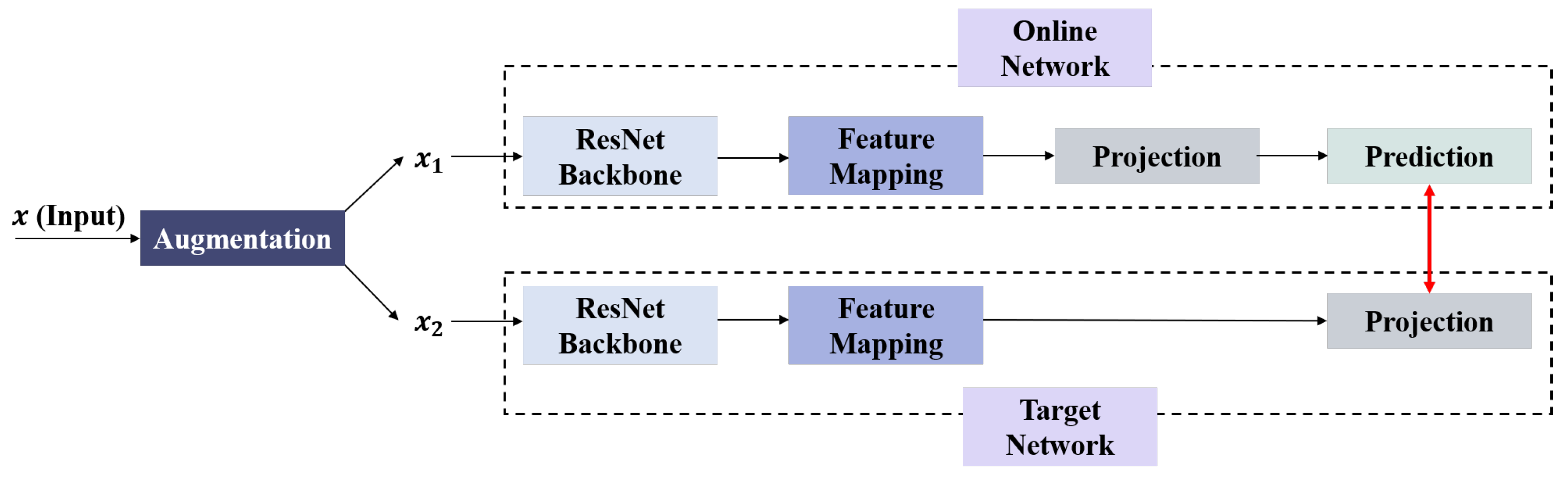
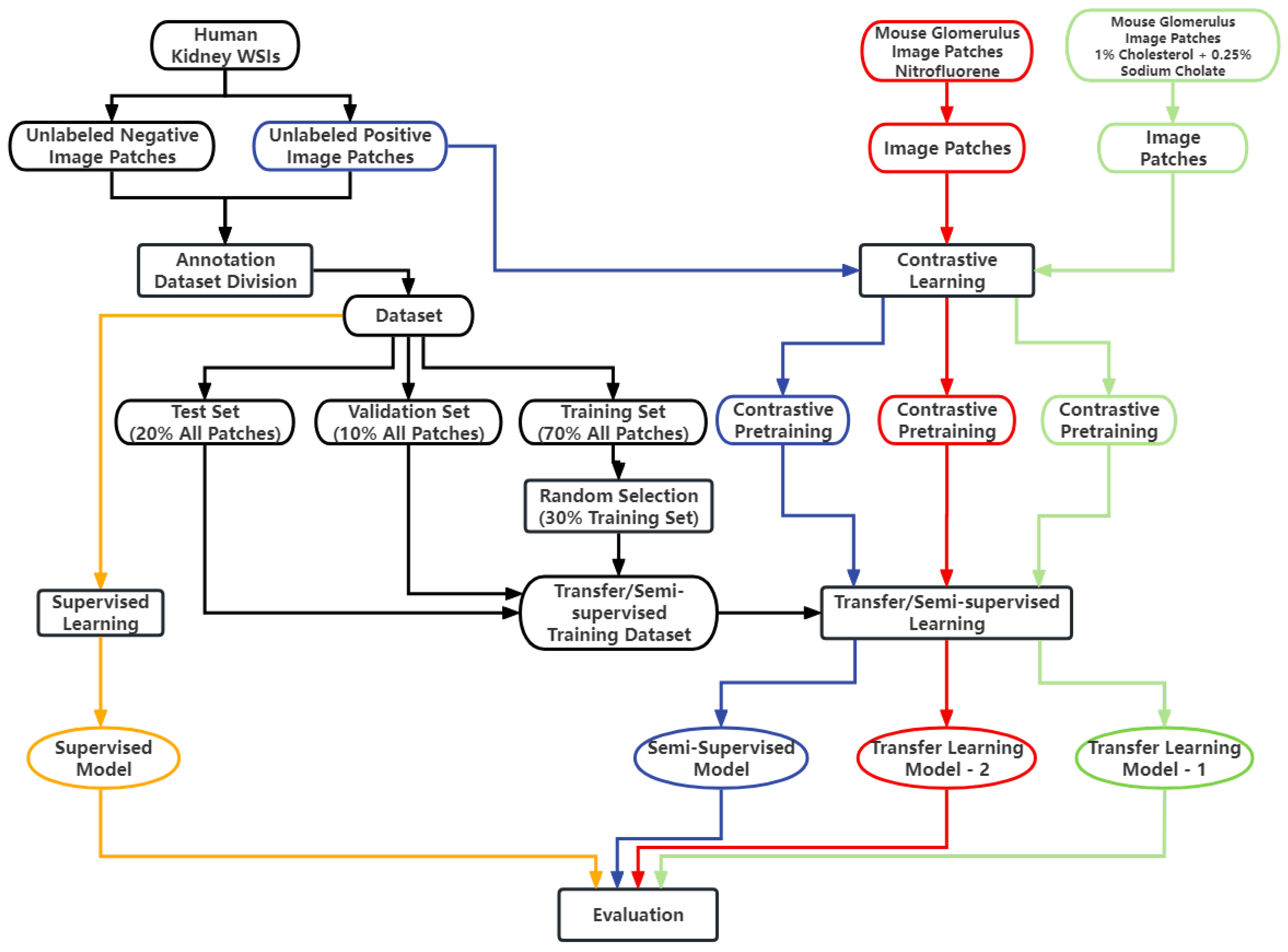
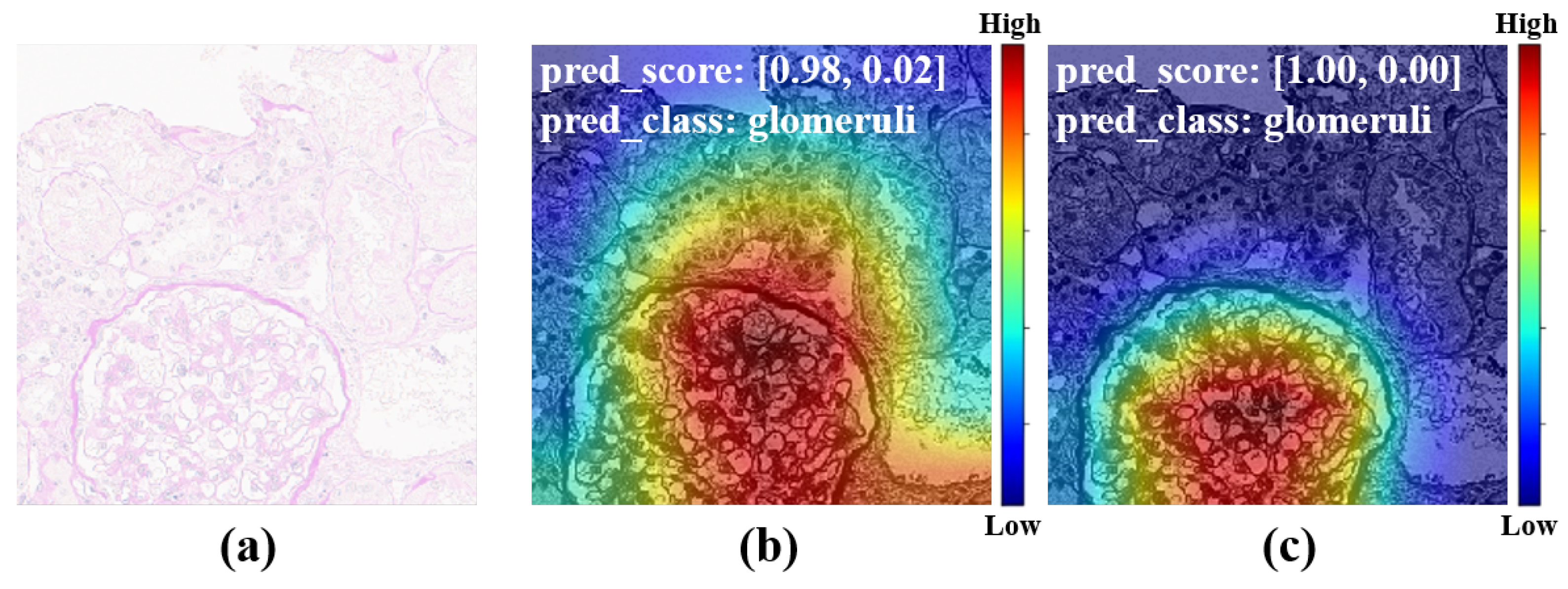
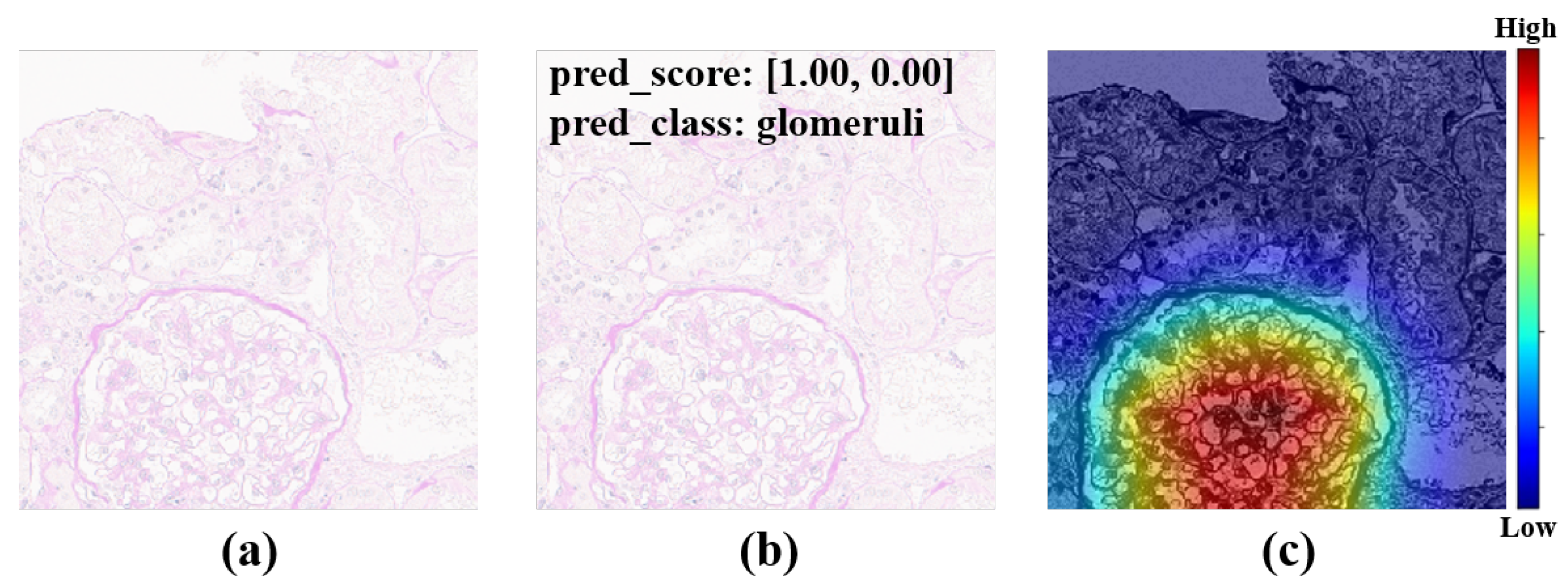
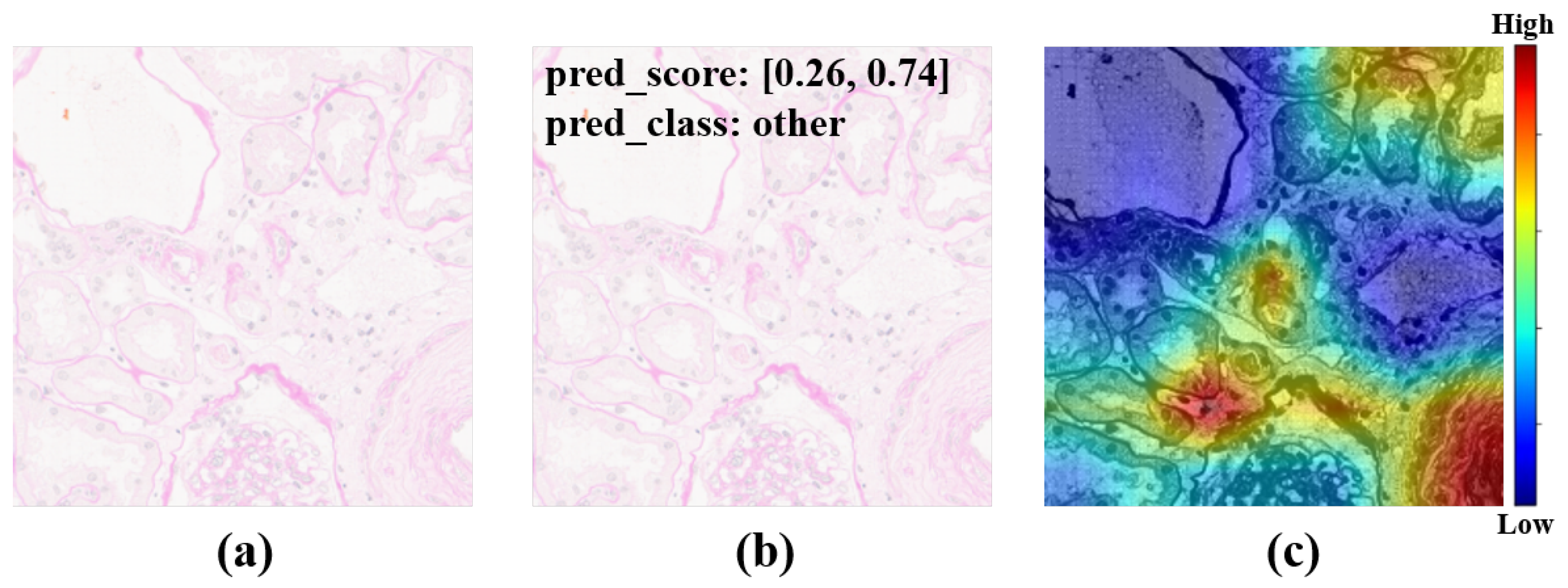
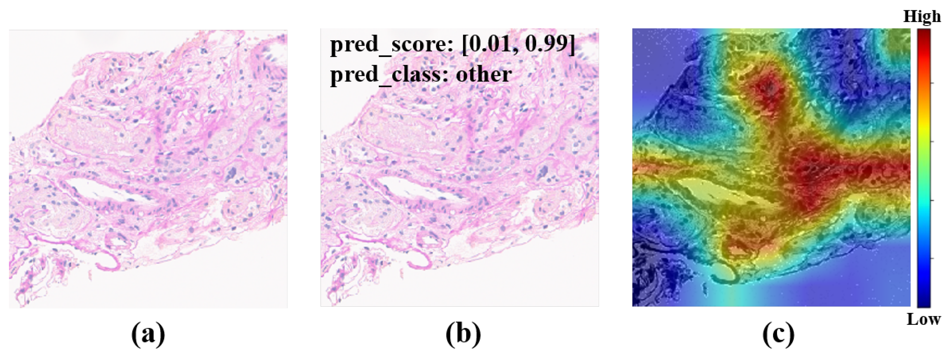
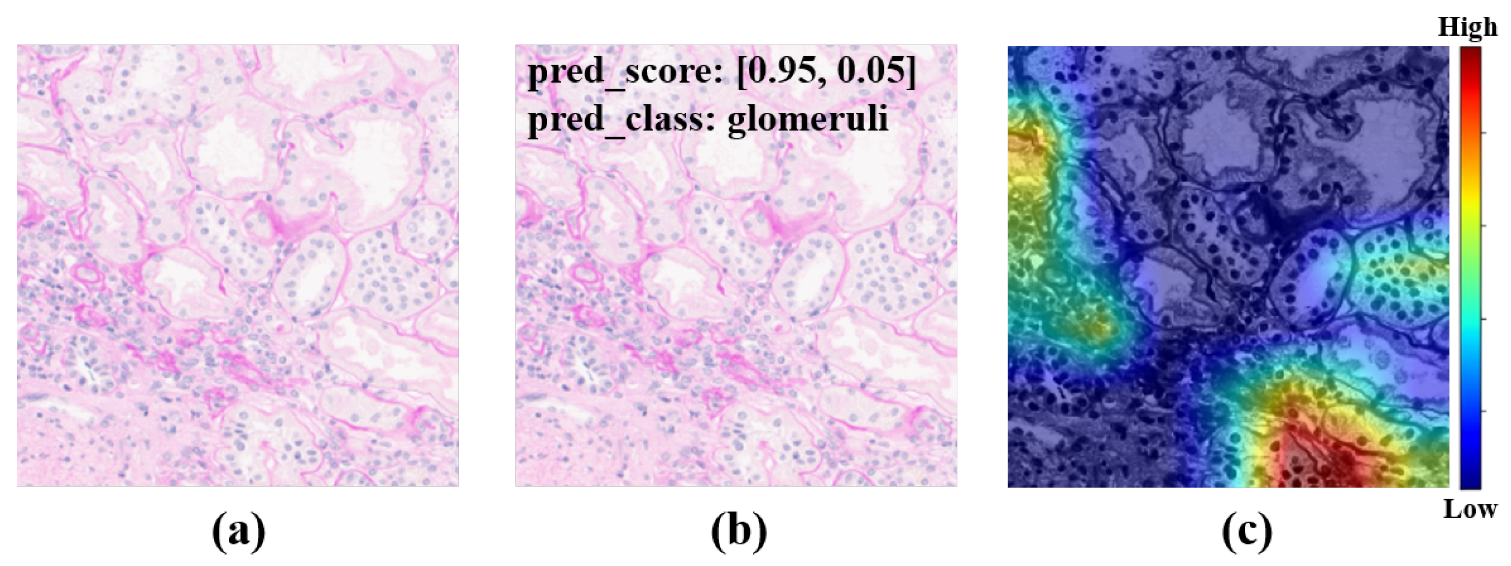
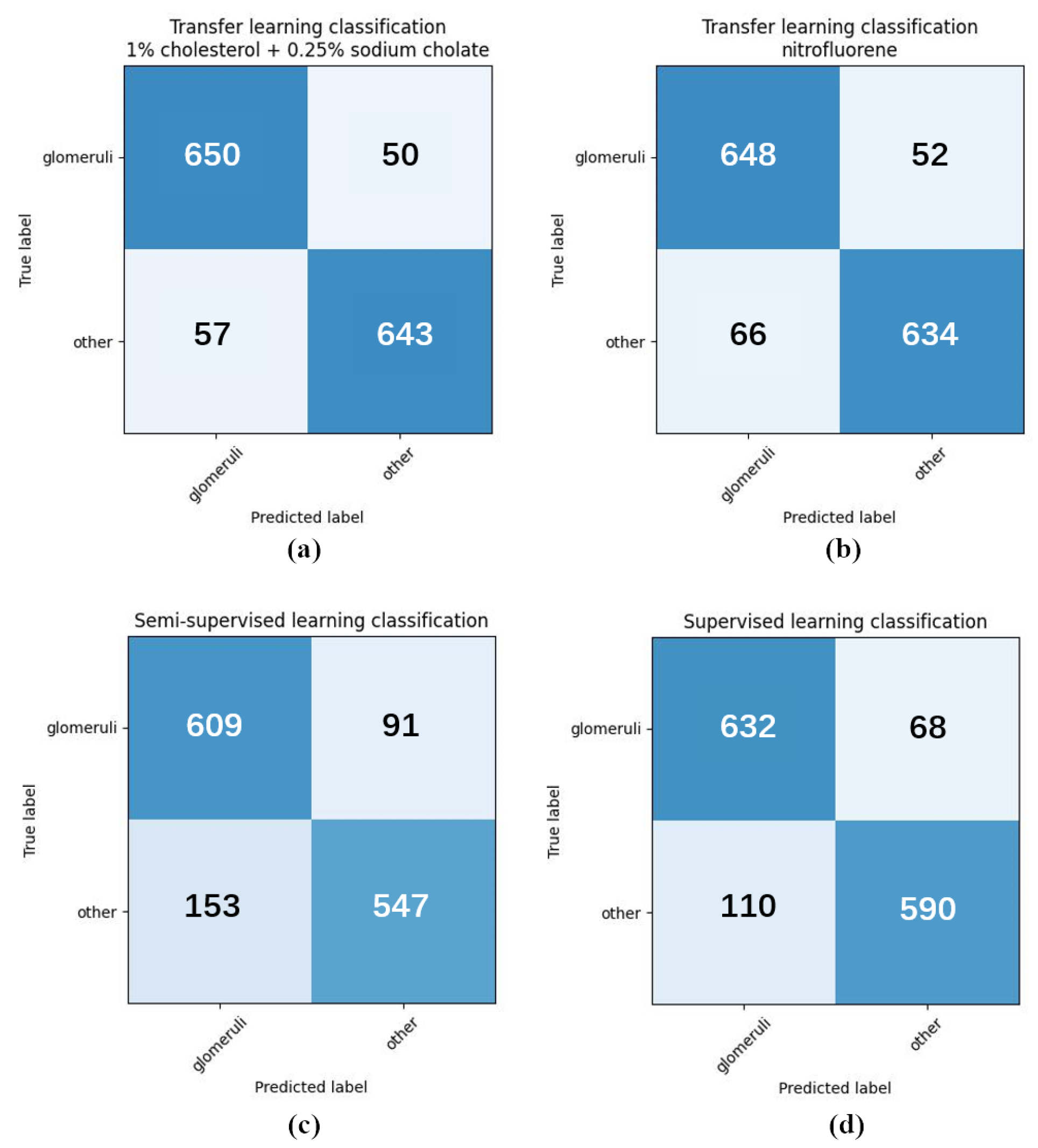
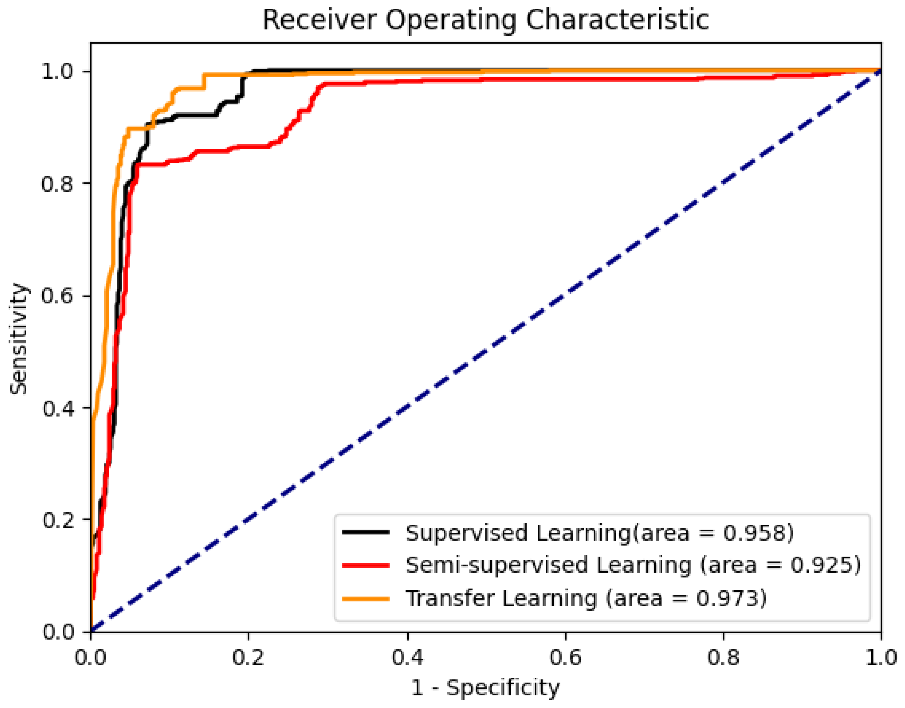
Semi-supervised learning can solve the above problems with a relatively low annotation cost. The classification performance of semi-supervised learning has been demonstrated in cases where the number of available annotated images is limited [50]. To achieve our goals, a large amount of unlabeled data were used for self-supervised pretraining, and then a small amount of labeled data were used for semi-supervised training. In total, 313 human IgA nephritis WSIs were processed into a human kidney image dataset, inclusive of 7000 glomerulus-containing (positive) images and 7000 non-glomerulus-containing (negative) images; 4900 patches containing human glomeruli were selected randomly for pretraining; the remaining 2100 patches containing glomeruli and 2100 randomly selected non-glomerulus patches were partitioned into training, validation, and test sets in a 7:1:2 ratio with classification labels for the fine-tuning phase. To minimize the dependence on negative images and capture stable glomerulus characteristics, contrastive pretraining was conducted with the BYOL algorithm. The feature representation of images containing glomeruli was obtained by enhancing the positive input with BYOL. The weights of the contrastive learning model were then fine-tuned to form a semi-supervised model. The proposed semi-supervised learning model achieved an average accuracy of 82.25%, a sensitivity of 80.78%, a specificity of 83.46%, and an AUROC of 0.925 in four parallel trials. The Grad-CAMs generated by this model showed that pretraining with contrastive learning based on positive images helps with the glomerulus image feature representation, and the areas associated with the glomeruli can provide a basis for correct predictions. In contrast, the supervised learning models based on the same dataset training and the same backbone were trained simultaneously. The supervised learning models achieved an average accuracy of 86.85%, a sensitivity of 87.48%, a specificity of 85.99%, and an AUROC of 0.958 in four parallel trials. The above results show that for IgA nephritis glomeruli, the semi-supervised classification model based on BYOL can achieve similar performance to that of the supervised learning classification model.

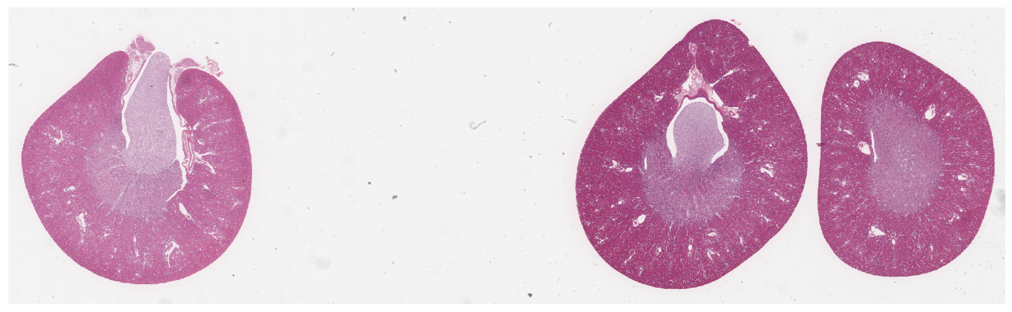
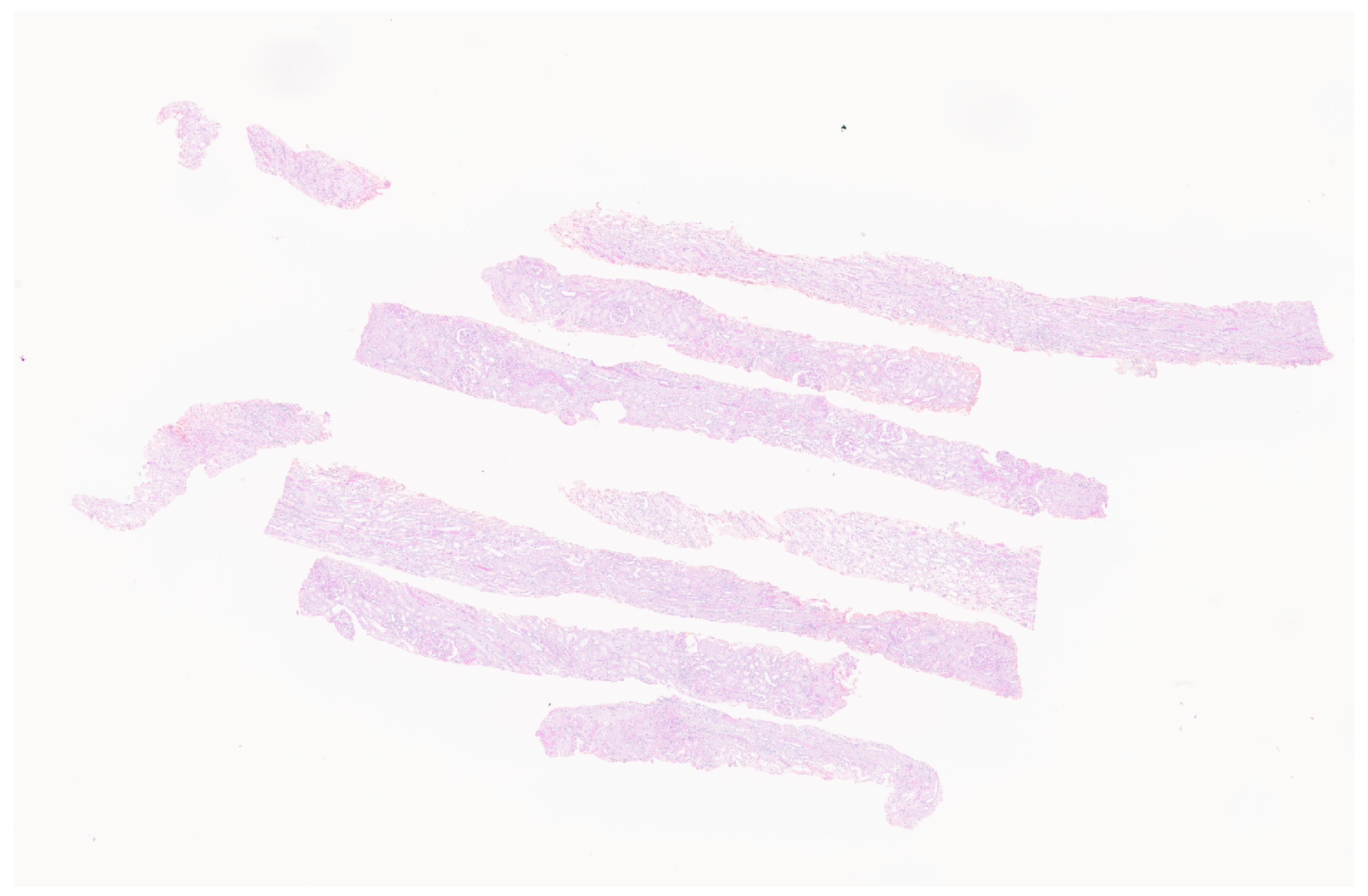
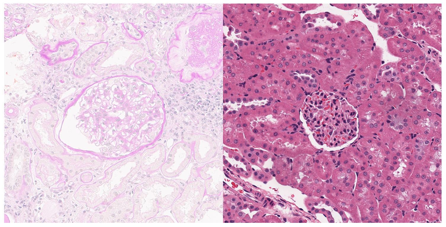
However, the supervised learning models still demonstrated obvious advantages through the Delong test analysis. This indicates that there is still room for improvement of classification models based on contrastive learning. In human kidney images, the morphology of other tissues that are not glomerulus might be similar to that of glomerulus. This implies that human kidney images may be more complex and may reduce the expressive effect of contrastive learning training. In mouse kidney images, the difference between glomerulus and other renal tissues is more significant, so the images are relatively simple. Given that the similarity between mouse glomeruli and human glomeruli is high, the same number of mouse glomerulus images could be introduced into contrastive learning to replace the human glomerulus images mentioned above. The same number of labeled human kidney images was then introduced for transfer training.

To train the transfer learning model, mouse dataset A was constructed with 5000 image patches containing mouse glomeruli affected by 1% cholesterol and 0.25% sodium cholate. To avoid drug-regimen differences in animal experiments, 5000 image patches containing mouse glomeruli affected by nitrofluorene comprised mouse dataset B for contrastive learning. Similar to the semi-supervised model training process described above, mouse datasets A and B were used for the contrastive learning phases, respectively. Then, 2100 patches containing human glomeruli and 2100 human non-glomerulus patches, both randomly selected, were partitioned into training, validation, and test sets in a 7:1:2 ratio with classification labels for the fine-tuning phase. The proposed transfer learning model with mouse dataset A achieved an average accuracy of 92.22%, a sensitivity of 92.74%, and a specificity of 91.58% in four parallel trials. The proposed transfer learning model with mouse dataset B achieved an average accuracy of 91.97%, a sensitivity of 92.56%, and a specificity of 91.21% in four parallel trials. The proposed transfer learning models achieved significant performance advantages under the Delong test, with an AUROC of 0.973, compared to the semi-supervised models and supervised models.

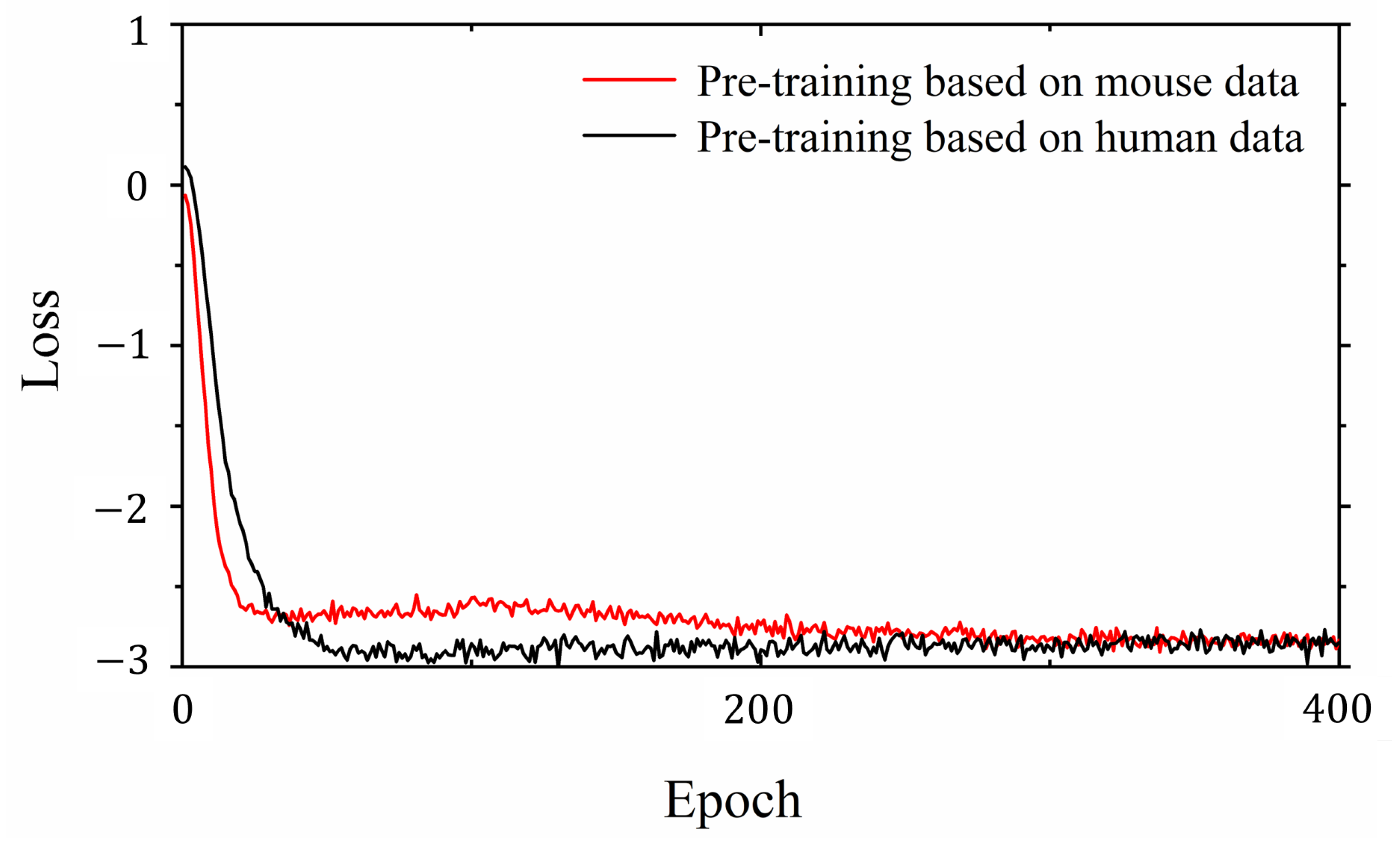
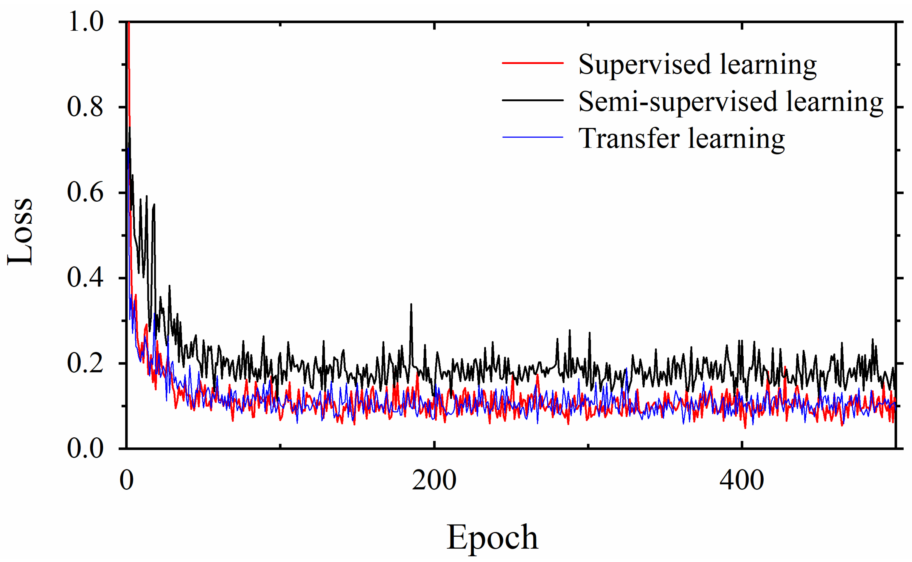
By comparing the loss curves of the above semi-supervised, supervised, and proposed transfer learning models, it was clear that when mouse glomerulus images were used for contrastive pretraining, the convergence speed was faster and the value of the loss function at convergence was lower. Observing the evaluation metrics and the confusion matrices of the two transfer learning models, the performance of the two transfer learning models was better than that of the semi-supervised learning model and the supervised learning model, and there was no significant difference in performance between the two transfer learning models. Comparing the previous results and Grad-CAMs, it was demonstrated that glomerulus images helped form better feature representations and improved the classification accuracy of human kidney images via transfer learning, surpassing the supervised learning methods. It can be demonstrated that the key to improving model performance lies in training the feature representations during the pretraining phase. The results of this study also show that semi-supervised learning and transfer learning models can be built using contrastive learning pretraining to improve the training results with small training datasets.

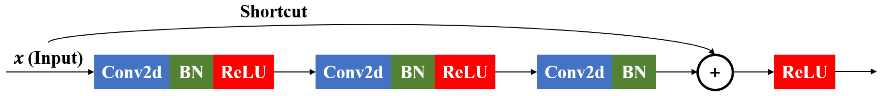
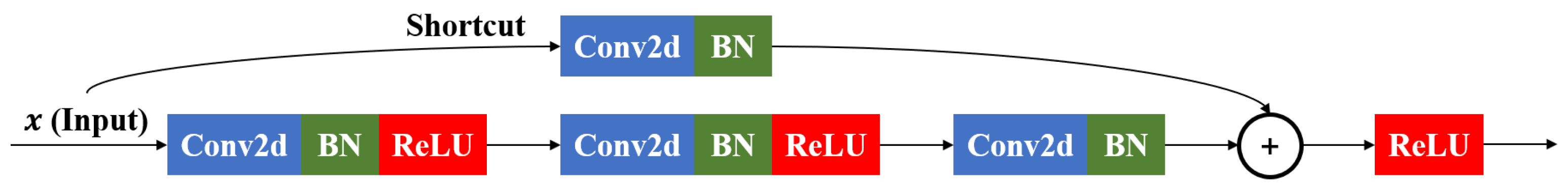
This study also examined the difference in the classification performance of the proposed transfer learning model with two ResNet backbones of different depths. This study confirmed the difference in the classification performance of the proposed transfer learning model with two ResNet backbones of different depths. With the same datasets, the transfer learning models based on ResNet-101 were trained and achieved an average classification accuracy of 92.73% in four parallel trials. Under the Delong test, the ResNet-101 backbone with an AUROC of 0.978 did not achieve a significant difference compared to that of the ResNet-50 backbone. This may be attributed to the simplicity of the mouse kidney images. Therefore, the ResNet-50 backbone has sufficient capability for feature learning and representation. Considering the storage and computational cost, the ResNet-50 backbone is more practical.

In this study, we proposed a classification model for analyzing human IgA nephritis WSIs by combining contrastive learning pretrained with mouse glomerulus images and transfer learning with human glomerulus images. The method achieved a high classification accuracy and facilitated the diagnosis using pathological WSI images. Additionally, the proposed method greatly reduced the requirement and burden of data annotation for training renal WSI analysis models. This study also provided a solid foundation for subsequent segmentation and classification tasks. There are some limitations of this study. First, this study only performed the classification of glomerulus and non-glomerulus tissue images and did not consider the classification for glomeruli and other tissues in different types of nephritis. The establishment of a comprehensive renal WSI-wide classification system is essential for a CAD system for chronic nephritis. Second, due to limitations in data collection, only mouse and human glomerulus images were used for pretraining by contrastive learning. The complexity and relationship between mouse and human glomerulus images have yet to be analyzed. In addition, the visualizations on the representation of features generated by mouse and human glomerulus images should be further studied. This may help to explain the role of contrastive learning in this study. Finally, the number of images in the dataset is insufficient to fully evaluate the performance of the models on large datasets. The evaluation of the model could be improved by incorporating a wider range of contrastive learning algorithms. BYOL is a generic contrastive learning algorithm, and its advantages over other algorithms have been extensively proved [23,31,51]. Future studies should be performed to develop a specific contrastive learning algorithm in renal pathological image analysis.

In future work, we will aim to address the above issues. The downstream tasks of the transfer learning classification model proposed in this study are also expected to progress, including multiclassification problems, detection, and semantic segmentation. In addition, we are approaching the application of transfer learning to downstream tasks in IgA nephritis, such as segmentation of internal sclerotic tissue, quantitative analysis of specific stained spots, and area statistics. WSIs with higher resolution and magnification can support this further study. Moreover, we would like to explore the feasibility of transfer learning with renal pathological images from appropriate animal experiments for the analysis of some rare glomerulus lesions, such as crescents. Additional data and models are expected to be available to address the problems identified above.

5. Conclusions

In this paper, the feasibility of a semi-supervised classification model was investigated based on contrastive learning for the detection of renal WSIs containing glomerulus, and a transfer learning model was also proposed based on the pretraining of mouse glomerulus images with high classification accuracy. A set of 313 IgA nephritis WSIs and two groups of mouse drug-experiment renal WSIs were used in this study. The proposed transfer learning model was compared with a semi-supervised learning model and a supervised learning model, both of which used the same classification backbone and dataset. The result shows that, with only mouse glomerulus images and a small number of IgA nephritis glomerulus images, the transfer learning method achieved 92.22% classification accuracy, outperforming the 86.85% classification accuracy of the supervised learning model.

References

1. Galla, J.H. IgA nephropathy. Kidney Int. 1995, 47, 377–387. [Google Scholar] [CrossRef] [PubMed]
2. Stachura, I.; Singh, G.; Whiteside, T.L. Immune abnormalities in IgA nephropathy (Berger’s disease). Clin. Immunol. Immunopathol. 1981, 20, 373–388. [Google Scholar] [CrossRef] [PubMed]
3. Schena, F.P.; Nistor, I. Epidemiology of IgA nephropathy: A global perspective. Semin. Nephrol. 2018, 38, 435–442. [Google Scholar] [CrossRef] [PubMed]
4. Korbet, S.M. Percutaneous renal biopsy. Semin. Nephrol. 2002, 22, 254–267. [Google Scholar] [CrossRef] [PubMed]
5. Fogo, A.B. Approach to renal biopsy. Am. J. Kidney Dis. 2003, 42, 826–836. [Google Scholar] [CrossRef] [PubMed]
6. Davidson, M.W.; Abramowitz, M. Optical microscopy. Encycl. Imaging Sci. Technol. 2002, 2, 120. [Google Scholar]
7. Barisoni, L.; Lafata, K.J.; Hewitt, S.M.; Madabhushi, A.; Balis, U.G. Digital pathology and computational image analysis in nephropathology. Nat. Rev. Nephrol. 2020, 16, 669–685. [Google Scholar] [CrossRef] [PubMed]
8. Ghaznavi, F.; Evans, A.; Madabhushi, A.; Feldman, M. Digital imaging in pathology: Whole-slide imaging and beyond. Annu. Rev. Pathol. Mech. Dis. 2013, 8, 331–359. [Google Scholar] [CrossRef]
9. Roberts, I.S. Pathology of IgA nephropathy. Nat. Rev. Nephrol. 2014, 10, 445–454. [Google Scholar] [CrossRef] [PubMed]
10. Liao, J.C.; Su, L.M. (Eds.) Advances in Image-Guided Urologic Surgery; Technical Report; Springer: Berlin/Heidelberg, Germany, 2015. [Google Scholar]
11. Barisoni, L.; Hodgin, J.B. Digital pathology in nephrology clinical trials, research, and pathology practice. Curr. Opin. Nephrol. Hypertens. 2017, 26, 450. [Google Scholar] [CrossRef] [PubMed]
12. Gallego, J.; Pedraza, A.; Lopez, S.; Steiner, G.; Gonzalez, L.; Laurinavicius, A.; Bueno, G. Glomerulus classification and detection based on convolutional neural networks. J. Imaging 2018, 4, 20. [Google Scholar] [CrossRef]
13. Uchino, E.; Suzuki, K.; Sato, N.; Kojima, R.; Tamada, Y.; Hiragi, S.; Yokoi, H.; Yugami, N.; Minamiguchi, S.; Haga, H.; et al. Classification of glomerular pathological findings using deep learning and nephrologist–AI collective intelligence approach. Int. J. Med. Inform. 2020, 141, 104231. [Google Scholar] [CrossRef] [PubMed]
14. Chagas, P.; Souza, L.; Araújo, I.; Aldeman, N.; Duarte, A.; Angelo, M.; Dos-Santos, W.L.; Oliveira, L. Classification of glomerular hypercellularity using convolutional features and support vector machine. Artif. Intell. Med. 2020, 103, 101808. [Google Scholar] [CrossRef] [PubMed]
15. Dimitri, G.M.; Andreini, P.; Bonechi, S.; Bianchini, M.; Mecocci, A.; Scarselli, F.; Zacchi, A.; Garosi, G.; Marcuzzo, T.; Tripodi, S.A. Deep learning approaches for the segmentation of glomeruli in kidney histopathological images. Mathematics 2022, 10, 1934. [Google Scholar] [CrossRef]
16. Gu, Y.; Ruan, R.; Yan, Y.; Zhao, J.; Sheng, W.; Liang, L.; Huang, B. Glomerulus Semantic Segmentation Using Ensemble of Deep Learning Models. Arab. J. Sci. Eng. 2022, 47, 14013–14024. [Google Scholar] [CrossRef]
17. Zhuang, F.; Qi, Z.; Duan, K.; Xi, D.; Zhu, Y.; Zhu, H.; Xiong, H.; He, Q. A comprehensive survey on transfer learning. Proc. IEEE 2020, 109, 43–76. [Google Scholar] [CrossRef]
18. Wang, W.; Lin, L.; Fan, Z.; Liu, J. Semi-supervised learning for mars imagery classification. In Proceedings of the 2021 IEEE International Conference on Image Processing (ICIP), Anchorage, AK, USA, 19–22 September 2021. [Google Scholar] [CrossRef]
19. Kato, S.; Oda, M.; Mori, K.; Shimizu, A.; Otake, Y.; Hashimoto, M.; Akashi, T. Classification and visual explanation for COVID-19 pneumonia from ct images using triple learning. Sci. Rep. 2022, 12, 20840. [Google Scholar] [CrossRef] [PubMed]
20. Wu, F.; Lin, H. Effect of transfer learning on the performance of vggnet-16 and resnet-50 for the classification of organic and residual waste. Front. Environ. Sci. 2022, 10, 1043843. [Google Scholar] [CrossRef]
21. Alzubaidi, L.; Al-Amidie, M.; Al-Asadi, A.; Humaidi, A.J.; Al-Shamma, O.; Fadhel, M.A.; Zhang, J.; Santamaría, J.; Duan, Y. Novel transfer learning approach for medical imaging with limited labeled data. Cancers 2021, 13, 1590. [Google Scholar] [CrossRef] [PubMed]
22. He, K.; Zhang, X.; Ren, S.; Sun, J. Deep residual learning for image recognition. In Proceedings of the IEEE Conference on Computer Vision and Pattern Recognition, Las Vegas, NV, USA, 27–30 June 2016; pp. 770–778. [Google Scholar]
23. Grill, J.B.; Strub, F.; Altché, F.; Tallec, C.; Richemond, P.; Buchatskaya, E.; Doersch, C.; Avila Pires, B.; Guo, Z.; Gheshlaghi Azar, M.; et al. Bootstrap your own latent-a new approach to self-supervised learning. Adv. Neural Inf. Process. Syst. 2020, 33, 21271–21284. [Google Scholar]
24. Igarashi, Y.; Nakatsu, N.; Yamashita, T.; Ono, A.; Ohno, Y.; Urushidani, T.; Yamada, H. Open TG-GATEs: A large-scale toxicogenomics database. Nucleic Acids Res. 2015, 43, D921–D927. [Google Scholar] [CrossRef] [PubMed]
25. Shoukat, A.; Akbar, S.; Hassan, S.A.; Iqbal, S.; Mehmood, A.; Ilyas, Q.M. Automatic diagnosis of glaucoma from retinal images using deep learning approach. Diagnostics 2023, 13, 1738. [Google Scholar] [CrossRef] [PubMed]
26. Masoudi, S.; Mehralivand, S.; Harmon, S.; Lay, N.; Lindenberg, L.; Mena, E.; Pinto, P.A.; Citrin, D.E.; Gulley, J.L.; Wood, B.J.; et al. Deep learning based staging of bone lesions from computed tomography scans. IEEE Access 2021, 9, 87531–87542. [Google Scholar] [CrossRef] [PubMed]
27. Kalbhor, M.; Shinde, S.; Popescu, D.; Hemanth, D.J. Hybridization of deep learning pre-trained models with machine learning classifiers and fuzzy min–max neural network for cervical cancer diagnosis. Diagnostics 2023, 13, 1363. [Google Scholar] [CrossRef] [PubMed]
28. He, K.; Zhang, X.; Ren, S.; Sun, J. Identity mappings in deep residual networks. In Proceedings of the Computer Vision–ECCV 2016: 14th European Conference, Amsterdam, The Netherlands, 11–14 October 2016; Springer: Berlin/Heidelberg, Germany, 2016; pp. 630–645. [Google Scholar]
29. Jang, E.; Gu, S.; Poole, B. Categorical reparameterization with gumbel-softmax. arXiv 2016, arXiv:1611.01144. [Google Scholar]
30. Richemond, P.H.; Grill, J.; Altché, F.; Tallec, C.; Strub, F.; Brock, A.; Smith, S.R.; De, S.; Pascanu, R.; Piot, B.; et al. Byol works even without batch statistics. arXiv 2020, arXiv:2010.10241. [Google Scholar] [CrossRef]
31. Qin, Y.; Ye, Y.; Zhao, Y.; Jian, W.; Zhang, H.; Cheng, K.; Li, K. Nearest neighboring self-supervised learning for hyperspectral image classification. Remote Sens. 2023, 15, 1713. [Google Scholar] [CrossRef]
32. Richemond, P.H.; Tam, A.; Tang, Y.; Strub, F.; Piot, B.; Hill, F. The edge of orthogonality: A simple view of what makes byol tick. arXiv 2023, arXiv:2302.04817. [Google Scholar] [CrossRef]
33. Bottou, L. Large-scale machine learning with stochastic gradient descent. In Proceedings of the COMPSTAT’2010: 19th International Conference on Computational Statistics, Paris, France, 22–27 August 2010; Springer: Berlin/Heidelberg, Germany, 2010; pp. 177–186. [Google Scholar]
34. Hardt, M.; Recht, B.; Singer, Y. Train faster, generalize better: Stability of stochastic gradient descent. In Proceedings of the International Conference on Machine Learning, PMLR, New York, NY, USA, 19–24 June 2016; pp. 1225–1234. [Google Scholar]
35. You, Y.; Li, J.; Reddi, S.; Hseu, J.; Kumar, S.; Bhojanapalli, S.; Song, X.; Demmel, J.; Keutzer, K.; Hsieh, C.J. Large batch optimization for deep learning: Training bert in 76 minutes. arXiv 2019, arXiv:1904.00962. [Google Scholar]
36. You, Y.; Gitman, I.; Ginsburg, B. Large batch training of convolutional networks. arXiv 2017, arXiv:1708.03888. [Google Scholar]
37. Xia, P.; Zhang, L.; Li, F. Learning similarity with cosine similarity ensemble. Inf. Sci. 2015, 307, 39–52. [Google Scholar] [CrossRef]
38. Contributors, M. OpenMMLab’s Pre-Training Toolbox and Benchmark. 2023. Available online: https://github.com/open-mmlab/mmpretrain (accessed on 15 June 2023).
39. Zhang, Z.; Sabuncu, M. Generalized cross entropy loss for training deep neural networks with noisy labels. In Proceedings of the Advances in Neural Information Processing Systems 31 (NeurIPS 2018), Montréal, QC, Canada, 3–8 December 2018. [Google Scholar]
40. Pang, T.; Xu, K.; Dong, Y.; Du, C.; Chen, N.; Zhu, J. Rethinking softmax cross-entropy loss for adversarial robustness. arXiv 2019, arXiv:1905.10626. [Google Scholar]
41. Gotmare, A.; Keskar, N.S.; Xiong, C.; Socher, R. A closer look at deep learning heuristics: Learning rate restarts, warmup and distillation. arXiv 2018, arXiv:1810.13243. [Google Scholar]
42. Carbonero-Ruz, M.; Martínez-Estudillo, F.J.; Fernández-Navarro, F.; Becerra-Alonso, D.; Martínez-Estudillo, A.C. A two dimensional accuracy-based measure for classification performance. Inf. Sci. 2017, 382, 60–80. [Google Scholar] [CrossRef]
43. Christen, P.; Hand, D.J.; Kirielle, N. A review of the F-measure: Its History, Properties, Criticism, and Alternatives. ACM Comput. Surv. 2023, 56, 1–24. [Google Scholar] [CrossRef]
44. Keilwagen, J.; Grosse, I.; Grau, J. Area under precision-recall curves for weighted and unweighted data. PLoS ONE 2014, 9, e92209. [Google Scholar] [CrossRef] [PubMed]
45. Hong, C.S.; Oh, T.G. TPR-TNR plot for confusion matrix. Commun. Stat. Appl. Methods 2021, 28, 161–169. [Google Scholar] [CrossRef]
46. Fawcett, T. An introduction to ROC analysis. Pattern Recognit. Lett. 2006, 27, 861–874. [Google Scholar] [CrossRef]
47. Hoo, Z.H.; Candlish, J.; Teare, D. What is an ROC curve? Emerg. Med. J. 2017, 34, 357–359. [Google Scholar] [CrossRef] [PubMed]
48. DeLong, E.R.; DeLong, D.M.; Clarke-Pearson, D.L. Comparing the areas under two or more correlated receiver operating characteristic curves: A nonparametric approach. Biometrics 1988, 44, 837–845. [Google Scholar] [CrossRef] [PubMed]
49. Selvaraju, R.R.; Cogswell, M.; Das, A.; Vedantam, R.; Parikh, D.; Batra, D. Grad-cam: Visual explanations from deep networks via gradient-based localization. In Proceedings of the IEEE International Conference on Computer Vision, Venice, Italy, 22–29 October 2017; pp. 618–626. [Google Scholar]
50. Boushehri, S.S.; Qasim, A.; Waibel, D.J.E.; Schmich, F.; Marr, C. Systematic comparison of incomplete-supervision approaches for biomedical imaging classification. Res. Sq. 2021, preprint. [Google Scholar] [CrossRef]
51. Garg, S.; Jain, D. Self-labeling refinement for robust representation learning with bootstrap your own latent. arXiv 2022, arXiv:2204.04545. [Google Scholar] [CrossRef]
Figure 1. An original WSI of a mouse kidney with an actual size of 75,695 × 22,500.
Electronics 13 01403 g001
Figure 2. An original WSI of a patient with IgA nephritis with an actual size of 35,856 × 23,388.
Electronics 13 01403 g002
Figure 3. WSI patches containing human (left) and mouse (right) glomerulus.
Electronics 13 01403 g003
Figure 4. The structure of the identity block.
Electronics 13 01403 g004
Figure 5. The structure of the convolutional block.
Electronics 13 01403 g005
Figure 6. The ResNet backbone with BYOL algorithm.
Electronics 13 01403 g006
Figure 7. Learning rate reduction strategy for contrastive learning.
Electronics 13 01403 g007
Figure 8. Learning rate reduction strategy for transfer learning.
Electronics 13 01403 g008
Figure 9. Data and experimental flow in this study. The blue stream represents semi-supervised learning training. The red and green streams represent transfer learning training with pretraining by mouse kidney images from different animal drug experiments. The orange stream represents supervised learning training used for comparison and evaluation.
Electronics 13 01403 g009
Figure 10. The training loss curves for contrastive pretraining. The red curve represents the training process using mouse glomerulus images, and the black curve represents the training process using human IgA nephritis glomerulus images.
Electronics 13 01403 g010
Figure 11. Training loss curves for semi-supervised learning (red), supervised learning (black), and transfer learning with mouse dataset A (blue).
Electronics 13 01403 g011
Figure 12. Accurate predictions of a positive image containing glomeruli. (a) is the original image patch. (b) is the Grad-CAM of the semi-supervised learning model. The model prediction is at the top, which comprises a binary group representing the positive and negative prediction scores, as is the prediction label. The first and second terms of the binary group represent the probability of a positive prediction (containing glomeruli) and a negative prediction (without glomeruli), respectively. (c) is the Grad-CAM of the transfer learning model. The model prediction scores and labels are also listed at the top.
Electronics 13 01403 g012
Figure 13. A correct prediction of a positive image containing glomeruli (true positive). (a) is the original image patch and labeled as a positive image. (b) has a positive prediction score of 1.00. (c) is the Grad-CAM of the prediction.
Electronics 13 01403 g013
Figure 14. An incorrect prediction of a positive image containing glomeruli. (a) is the original image patch and labeled as a positive image. (b) has a positive prediction score of 0.26. (c) is the Grad-CAM of the positive prediction.
Electronics 13 01403 g014
Figure 15. A correct prediction of a negative image without glomeruli. (a) is the original image patch and labeled as a negative image. (b) has a negative prediction score of 0.99. (c) is the Grad-CAM of the prediction.
Electronics 13 01403 g015
Figure 16. An incorrect prediction of a negative image containing glomeruli. (a) is the original image patch and labeled as a positive image. (b) has a negative prediction score of 0.05. (c) is the Grad-CAM of the prediction.
Electronics 13 01403 g016
Figure 17. Confusion matrices of two transfer learning models (a,b), the supervised learning model (c), and the semi-supervised learning model (d), respectively.
Electronics 13 01403 g017
Figure 18. The ROC and AUROC of the 3 different models. The orange curve represents the transfer learning model of mouse dataset A with an AUROC of 0.973. The black curve represents the supervised learning model with an AUROC of 0.958. The red curve represents the semi-supervised learning model with an AUROC of 0.925. The dotted line represents a random classifier.
Electronics 13 01403 g018