
A Method to Track Moving Targets Using a Doppler Radar Based on Converted State Kalman Filtering
Abstract
:1. Introduction
2. Description of Problem
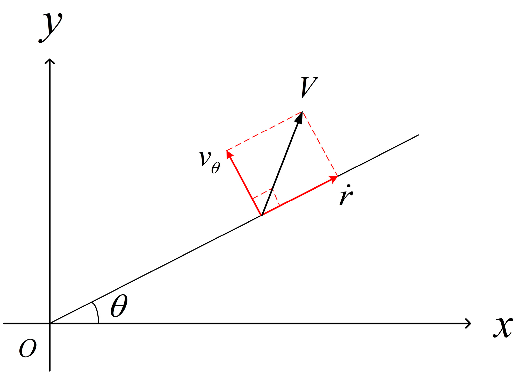
2.1. Decomposition of Motion
2.2. Target Motion Equations in the Polar Coordinate System
2.2.1. CV Motion
2.2.2. CA Motion
3. Converted State Kalman Filtering with Doppler Measurement
3.1. Measurement Equations with Doppler Measurement
3.2. Analysis of Process Noise
- (1)
- The 2n + 1 sigma sample points (n is the state dimension) are generated based on the mean and variance of the three-dimensional random vector (CV motion) or (CA motion).
- (2)
- The sigma sample points are then substituted into Equation (13) to calculate the sample points generated via nonlinear mapping.
- (3)
- Through the weighted sum, we obtained the mean and variance of the process noise (CV motion) or (CA motion) in the polar coordinate system.
3.3. CSKF Algorithm with Doppler Measurement
- (1)
- We predict the system state and covariance.
- (2)
- Then, Kalman gain is calculated.
- (3)
- Finally, we update the system state and covariance.
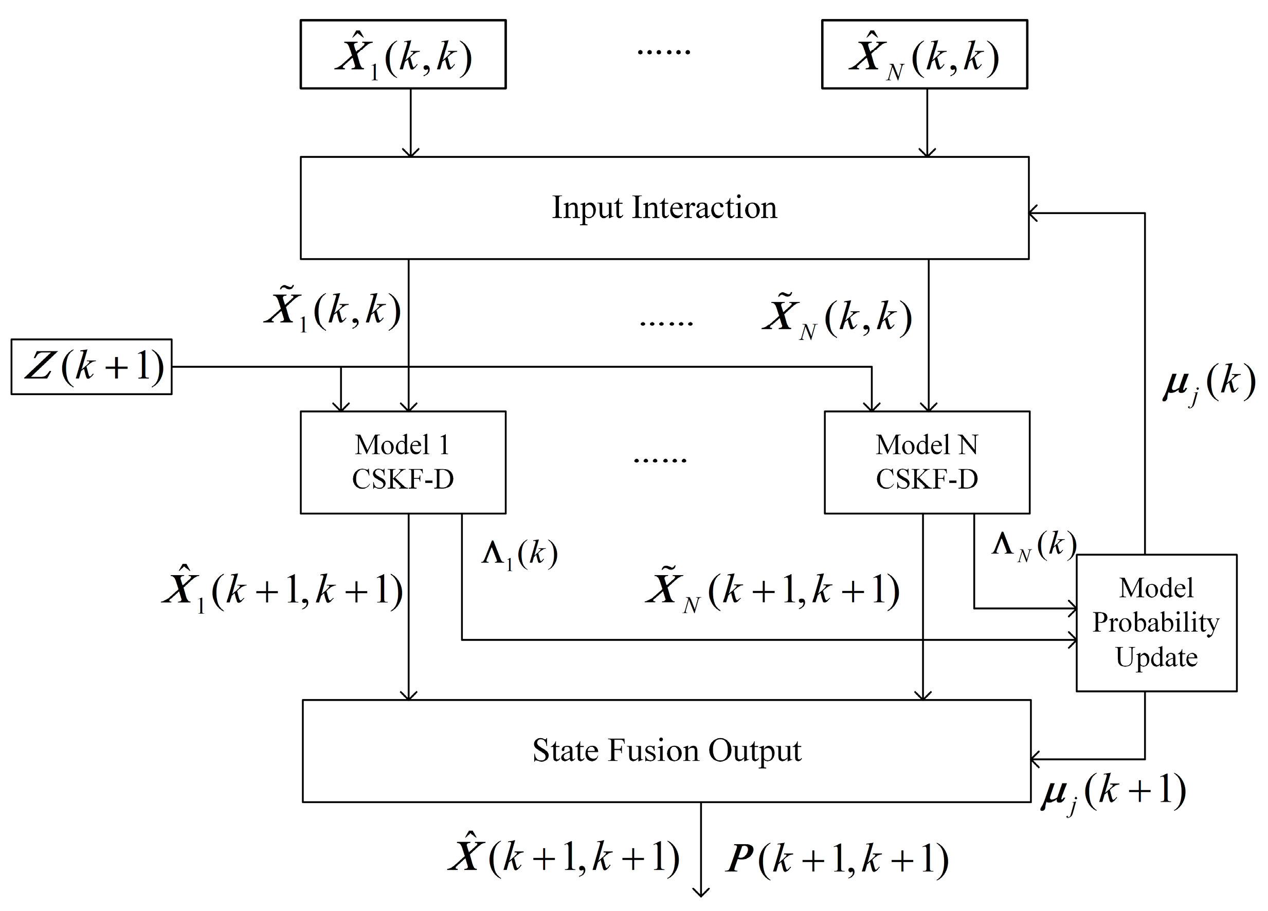
4. Target Tracking with Combined CSKF-D and IMM Method
- (1)
- Input interaction:where is the mixed transition probability; , where represents the model probability of model of the target at time ; and represents the transition probability from model to model . and , respectively, represent the state estimate of the target model at time and its covariance matrix. and , respectively, represent the state interaction value of the target model at time and its covariance matrix.
- (2)
- State filtering: and are used as filter inputs to obtain the state estimate and covariance matrix at the next moment. Section 3.3 of this manuscript describes the single model filtering algorithm process.
- (3)
- Model probability update:where is the normalization constant.where and are the predicated state and covariance of the target at time ; and are the measurement residuals and their covariances. Therefore, our model is directly derived from the difference between observations and linear predictions in the residual calculation. As a result, our model is free of nonlinear approximation errors, which makes it capable of yielding more accurate model probabilities.
- (4)
- State fusion output: Based on the posterior probability of each model, a probability-weighted summation of the state estimates of each filter obtains the final estimated state and covariance estimate.
5. Simulation Results and Analysis
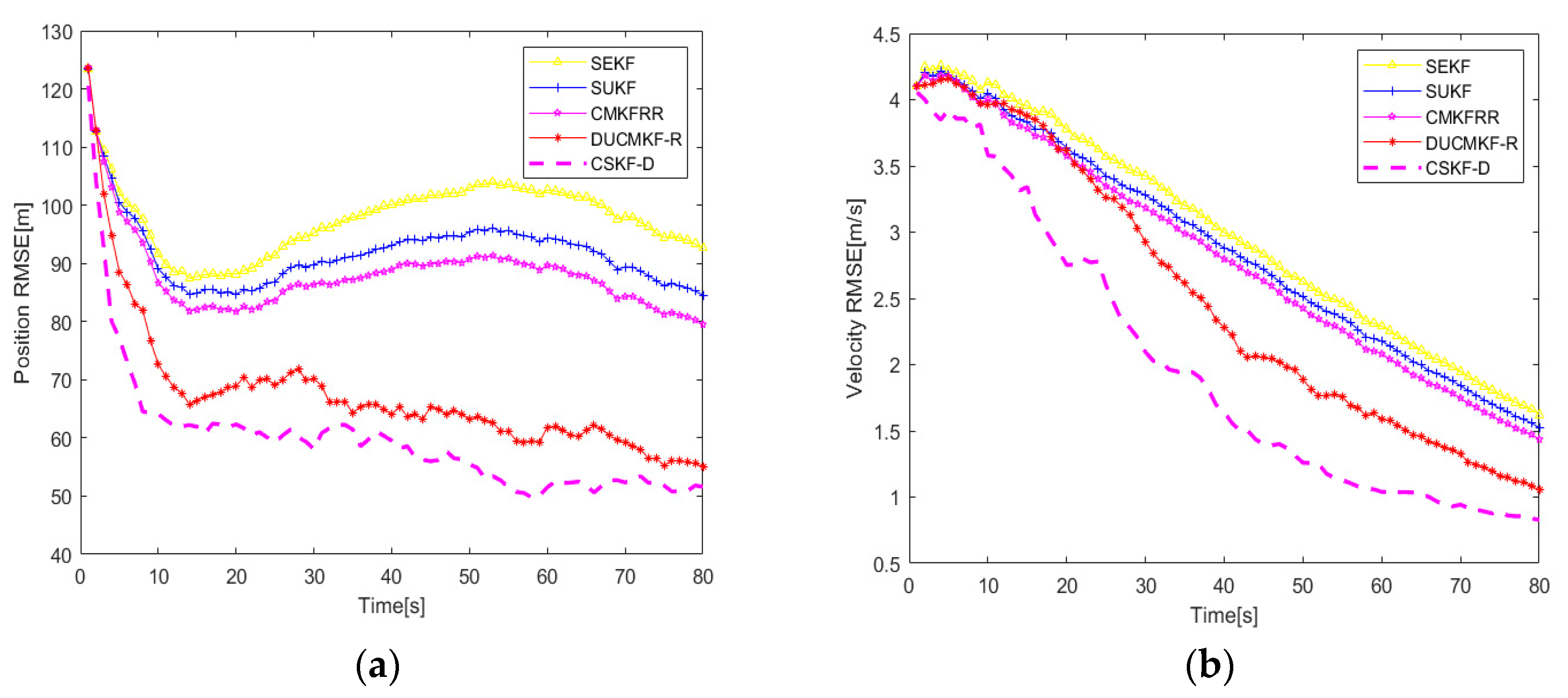
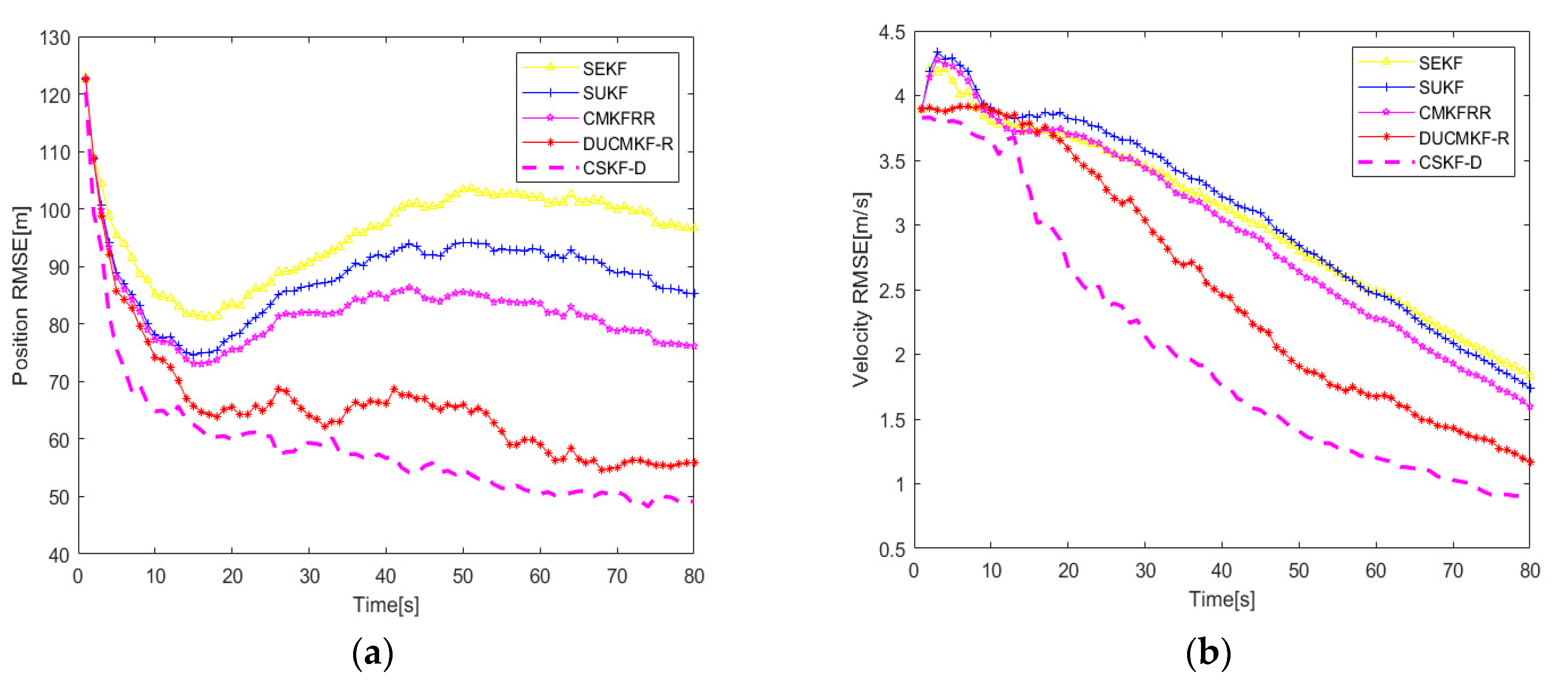
5.1. CV Model
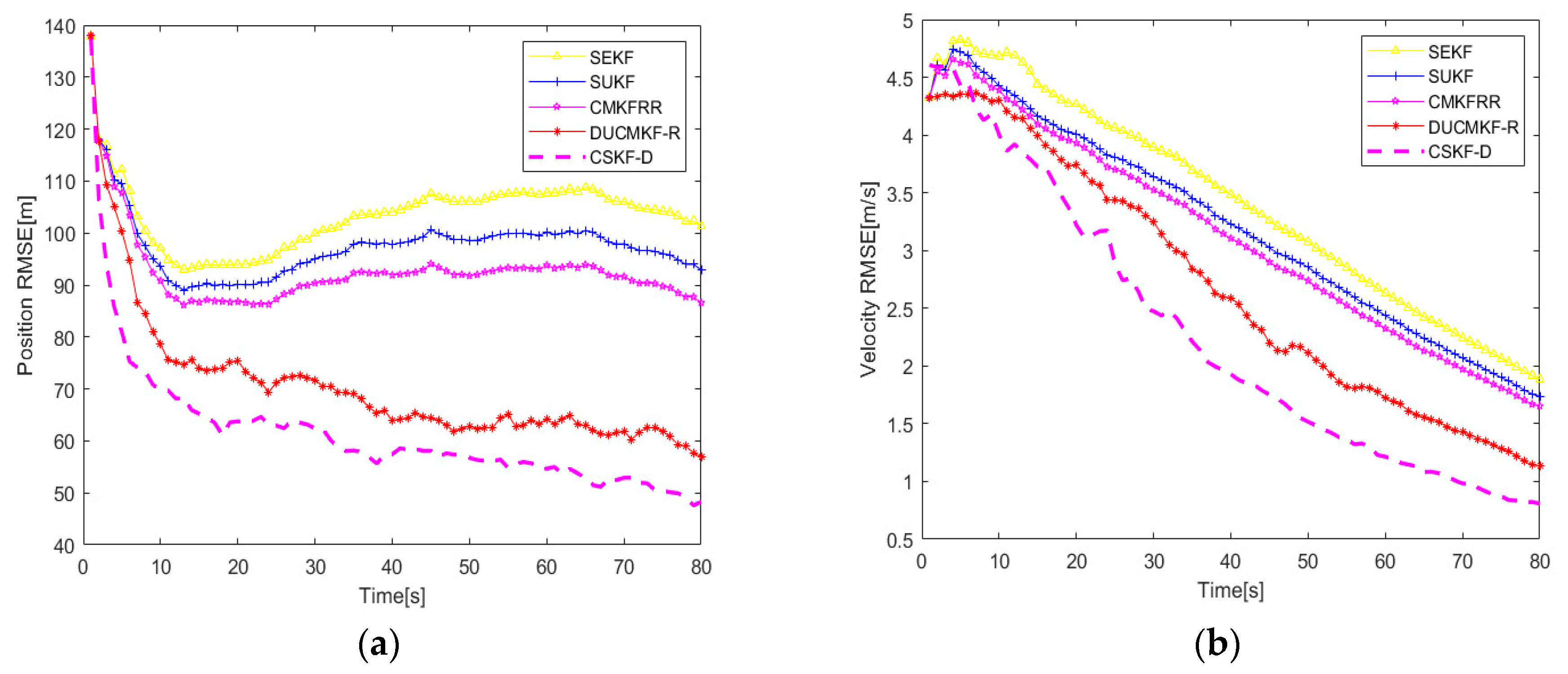
5.2. CA Model
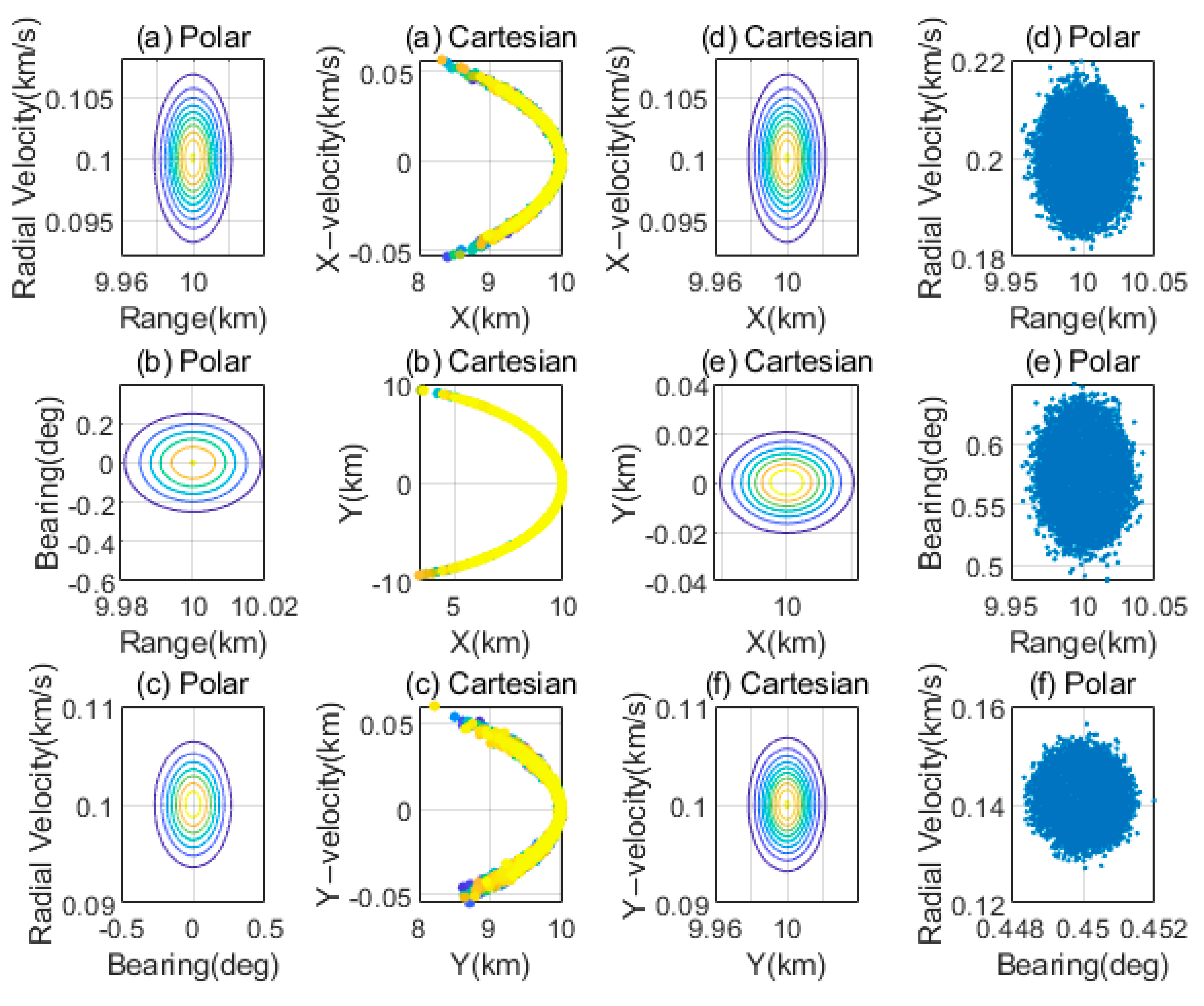
- (1)
- From polar coordinates to Cartesian coordinates, we deduce the following:
- (2)
- The following equation is deduced from Cartesian coordinates to polar coordinates:where , , , and are the valid positions and velocities, respectively, in the Cartesian coordinate system. Moreover, , , , and are the true range, radial velocity, bearing, and tangential velocity, respectively, in the polar coordinate system. and are the zero-mean Gaussian noises with covariances and , respectively.
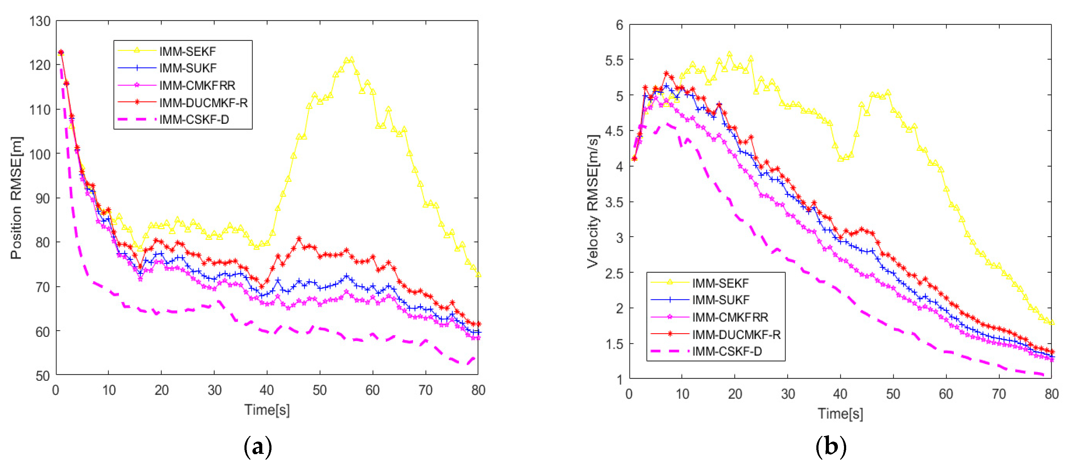
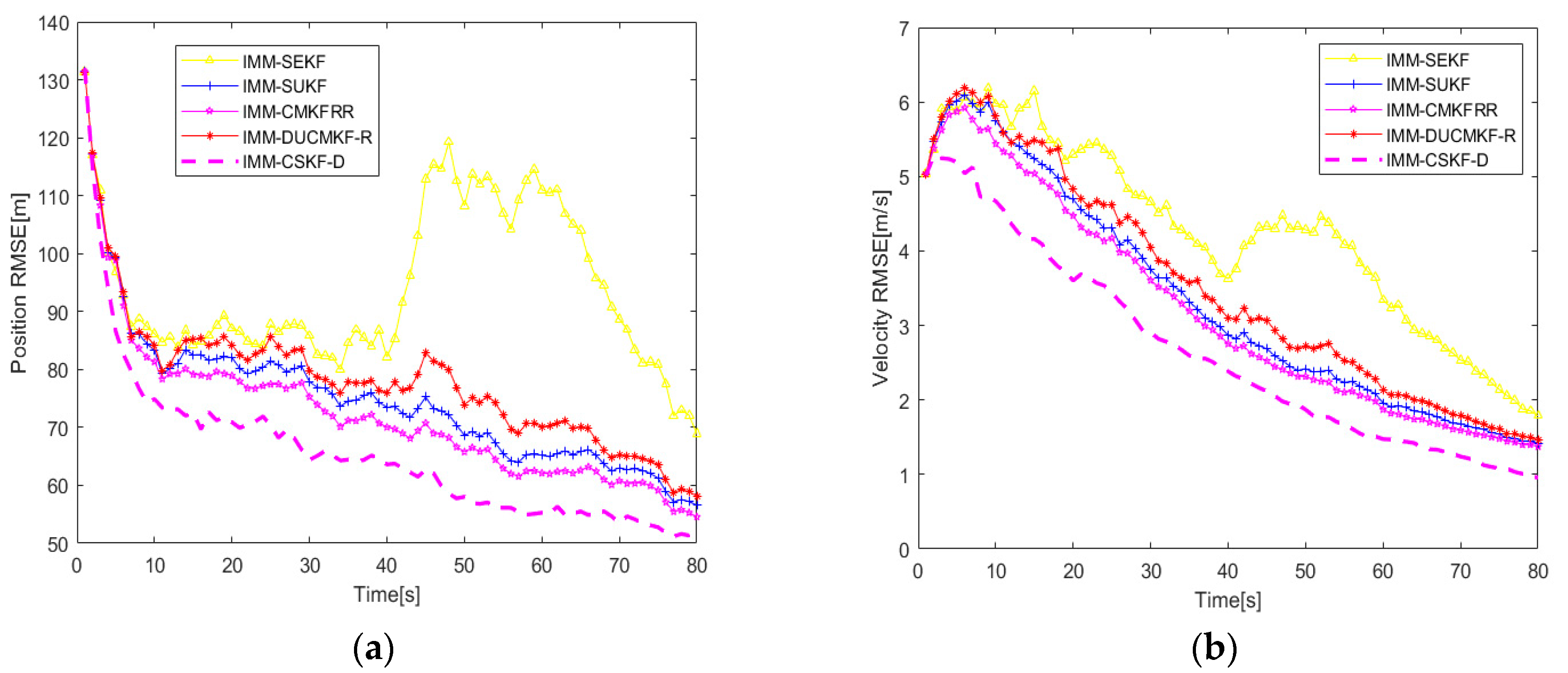
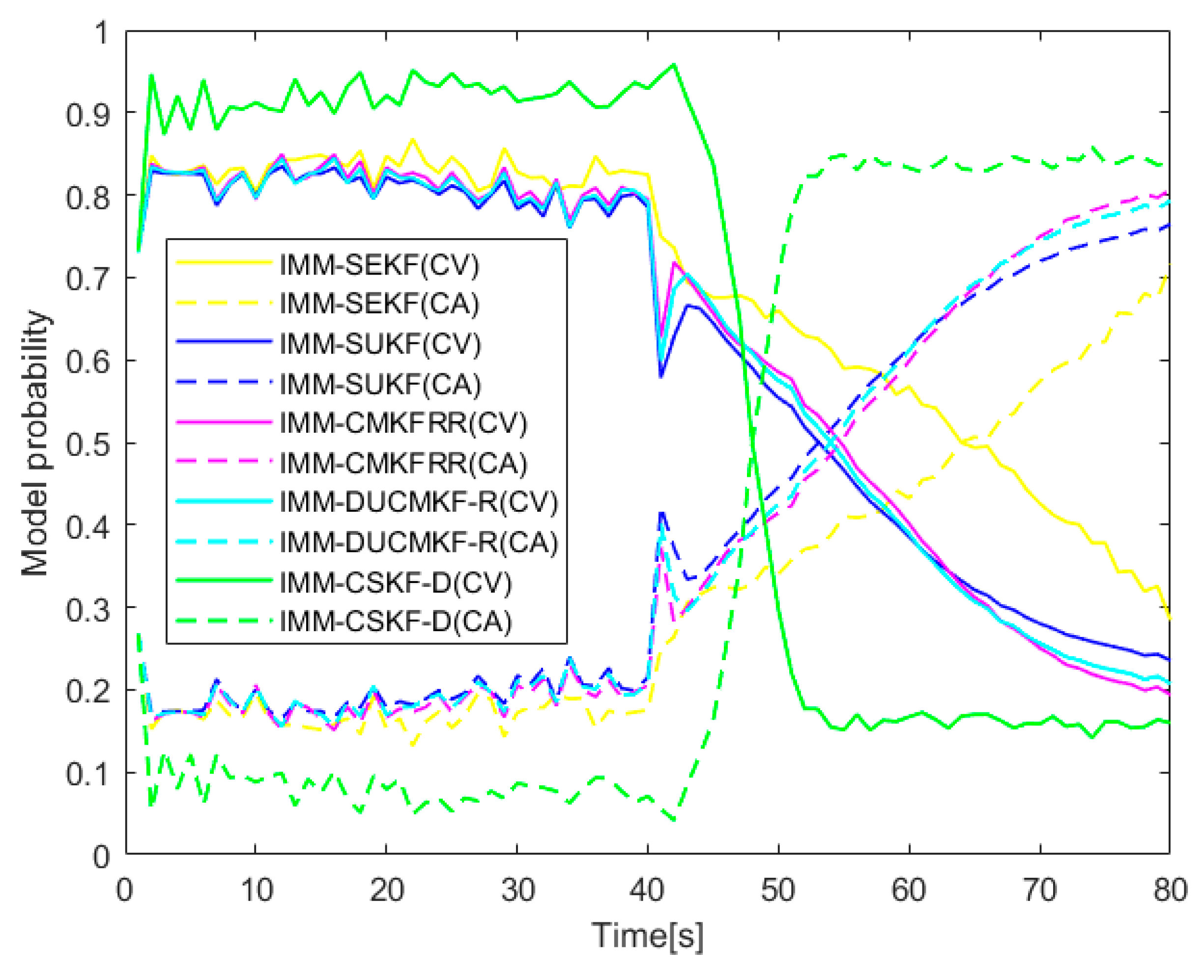
5.3. IMM Model
6. Conclusions
Author Contributions
Funding
Data Availability Statement
Conflicts of Interest
References
- Wang, X.; Musicki, D.; Ellem, R.; Fletcher, F. Efficient and enhanced multi-target tracking with Doppler measurements. IEEE Trans. Aerosp. Electron. Syst. 2009, 45, 1400–1417. [Google Scholar] [CrossRef]
- Li, S.; Cheng, Y.; Wang, H.; Gao, S. Distributed multisensor multitarget tracking algorithm with time-offset registration. J. Northwestern Polytech. Univ. 2020, 38, 797–805. [Google Scholar] [CrossRef]
- Smith, M.A. On Doppler measurements for tracking. In Proceedings of the 2008 International Conference on Radar, Adelaide, Australia, 2–5 September 2008; pp. 513–518. [Google Scholar] [CrossRef]
- Zhou, G.; Guo, Z.; Li, K.; Wu, L. Motion modeling and state estimation in range-Doppler plane. Aerosp. Sci. Technol. 2021, 115, 106792. [Google Scholar] [CrossRef]
- Wang, J.G.; Long, T.; He, P.K. A new method of incorporating radial velocity measurement into Kalman filter. Proc. Signal Process. 2002, 18, 414–416. [Google Scholar] [CrossRef]
- Saha, M.; Ghosh, R.; Goswami, B. Robustness and sensitivity metrics for tuning the extended Kalman filter. IEEE Trans. Instrum. Meas. 2013, 63, 964–971. [Google Scholar] [CrossRef]
- Lee, H.; Chun, J.; Jeon, K. Experimental results and posterior cramér–rao bound analysis of EKF-based radar SLAM with odometer bias compensation. IEEE Trans. Aerosp. Electron. Syst. 2020, 57, 310–324. [Google Scholar] [CrossRef]
- Kaba, U.; Temeltas, H. Generalized bias compensated pseudolinear Kalman filter for colored noisy bearings-only measurements. Signal Process. 2022, 190, 108331. [Google Scholar] [CrossRef]
- Duan, Z.; Han, C. Radar Target Tracking with Doppler Measurements in Polar Coordinates. J. Syst. Simul. 2004, 16, 2860–2863. [Google Scholar] [CrossRef]
- Jiao, L.; Pan, Q.; Liang, Y.; Yang, F. A nonlinear tracking algorithm with range-rate measurements based on unbiased measurement conversion. In Proceedings of the 2012 15th International Conference on Information Fusion, Singapore, 9–12 July 2012; pp. 1400–1405. [Google Scholar]
- Lerro, D.; Bar-Shalom, Y. Tracking with debiased consistent converted measurements versus EKF. IEEE Trans. Aerosp. Electron. Syst. 1993, 29, 1015–1022. [Google Scholar] [CrossRef]
- Bordonaro, S.V.; Willett, P.; Bar-Shalom, Y.; Luginbuhl, T. Converted measurement sigma point Kalman filter for bistatic sonar and radar tracking. IEEE Trans. Aerosp. Electron. Syst. 2018, 55, 147–159. [Google Scholar] [CrossRef]
- Wang, K.; Li, X.; Wu, P.; He, S. A modified unbiased converted measurement target tracking algorithm based on expectation maximization. J. Aeronaut. Astronaut. Aviat. 2021, 53, 497–509. [Google Scholar]
- Wang, G.; Feng, X. Unbiased converted measurement manoeuvering target tracking under maximum correntropy criterion. Cogn. Comput. Syst. 2020, 2, 125–129. [Google Scholar] [CrossRef]
- Li, K.; Zhou, G.; Cui, N. Motion Modeling and State Estimation in Range-Squared Coordinate. IEEE Trans. Signal Process. 2022, 70, 5279–5294. [Google Scholar] [CrossRef]
- Mo, L.; Song, X.; Zhou, Y.; Sun, Z.K.; Yaakov, B.-S. Unbiased converted measurements for tracking. IEEE Trans. Aerosp. Electron. Syst. 1998, 34, 1023–1027. [Google Scholar]
- Duan, Z.; Li, X.R.; Han, C.; Zhu, H. Sequential unscented Kalman filter for radar target tracking with range rate measurements. In Proceedings of the 2005 7th International Conference on Information Fusion, Philadelphia, PA, USA, 25–28 July 2005; pp. 1–8. [Google Scholar] [CrossRef]
- Kandepu, R.; Foss, B.; Imsland, L. Applying the unscented Kalman filter for nonlinear state estimation. J. Process Control 2008, 18, 753–768. [Google Scholar] [CrossRef]
- Julier, S.J.; Uhlmann, J.K. Unscented filtering and nonlinear estimation. Proc. IEEE 2004, 92, 401–422. [Google Scholar] [CrossRef]
- Kulikov, G.Y.; Kulikova, M.V. Square-root accurate continuous-discrete extended-unscented Kalman filtering methods with embedded orthogonal and J-orthogonal QR decompositions for estimation of nonlinear continuous-time stochastic models in radar tracking. Signal Process. 2020, 166, 107253. [Google Scholar] [CrossRef]
- Guo, Z.; Zhou, G. State estimation from range-only measurements. In Proceedings of the 2020 IEEE 23rd International Conference on Information Fusion (FUSION), Rustenburg, South Africa, 6–9 July 2020; pp. 1–6. [Google Scholar] [CrossRef]
- Zhou, G.; Pelletier, M.; Kirubarajan, T.; Quan, T. Statically fused converted position and Doppler measurement Kalman filters. IEEE Trans. Aerosp. Electron. Syst. 2014, 50, 300–318. [Google Scholar] [CrossRef]
- Li, S.; Icheng, T. Interactive multiple model algorithm for a doppler radar maneuvering target tracking based on converted measurements. Acta Electron. Sin. 2019, 47, 538–544. [Google Scholar]
- Bordonaro, S.; Willett, P.; Bar-Shalom, Y. Consistent linear tracker with converted range, bearing, and range rate measurements. IEEE Trans. Aerosp. Electron. Syst. 2017, 53, 3135–3149. [Google Scholar] [CrossRef]
- Liu, H.; Zhou, Z.; Yu, L.; Lu, C. Two unbiased converted measurement Kalman filtering algorithms with range rate. IET Radar Sonar Navig. 2018, 12, 1217–1224. [Google Scholar] [CrossRef]
- Zhang, W.; Zhao, X.; Liu, Z.; Liu, K.; Chen, B. Converted state equation Kalman filter for nonlinear maneuvering target tracking. Signal Process. 2023, 202, 108741. [Google Scholar] [CrossRef]
- Yang, C.; Ke, Z.; Meibai, L. Exploring a better IMM-UKF fusion algorithm based on current statistical model in target tracking. J. Northwestern Polytech. Univ. 2011, 29, 919–926. [Google Scholar]
- Liu, Q.; Yang, X. Improved interacting multiple model particle filter algorithm. J. Northwestern Polytech. Univ. 2018, 36, 169–175. [Google Scholar] [CrossRef]
- Zhang, Z.; Zhou, G. Maneuvering target state estimation based on separate modeling with B-splines. Aerosp. Sci. Technol. 2022, 119, 107172. [Google Scholar] [CrossRef]


| Scenario | |||
|---|---|---|---|
| 1 | 50 | 0.5 | 0.05 |
| 2 | 100 | 1 | 0.1 |
| Measurement Noise Parameters | Method | RMSE of Position (m) | RMSE of Velocity (m/s) |
|---|---|---|---|
| SEKF | 99.14 | 2.87 | |
| SUKF | 93.96 | 2.69 | |
| CMKFRR | 89.35 | 2.53 | |
| DUCMKF-R | 72.74 | 2.37 | |
| CSKF-D | 61.86 | 1.83 | |
| SEKF | 111.24 | 3.44 | |
| SUKF | 102.96 | 3.26 | |
| CMKFRR | 97.62 | 3.17 | |
| DUCMKF-R | 75.54 | 2.97 | |
| CSKF-D | 62.33 | 2.34 |
| Measurement Noise Parameters | Method | RMSE of Position (m) | RMSE of Velocity (m/s) |
|---|---|---|---|
| SEKF | 100.54 | 2.94 | |
| SUKF | 92.41 | 2.73 | |
| CMKFRR | 89.23 | 2.61 | |
| DUCMKF-R | 71.85 | 2.42 | |
| CSKF-D | 61.17 | 1.97 | |
| SEKF | 112.53 | 3.50 | |
| SUKF | 103.69 | 3.24 | |
| CMKFRR | 98.50 | 3.21 | |
| DUCMKF-R | 79.54 | 2.89 | |
| CSKF-D | 62.87 | 2.57 |
| Scenario 1 | Scenario 2 | Scenario 3 | |
|---|---|---|---|
| Cartesian coordinates | |||
| Polar coordinates |
| Scenario | |||
|---|---|---|---|
| 1 | 60 | 0.6 | 0.06 |
| 2 | 120 | 1.2 | 0.12 |
| Measurement Noise Parameters | Method | RMSE of Position (m) | RMSE of Velocity (m/s) |
|---|---|---|---|
| IMM-SEKF | 94.67 | 3.97 | |
| IMM-SUKF | 81.70 | 3.08 | |
| IMM-CMKFRR | 78.87 | 2.94 | |
| IMM-DUCMKF-R | 76.34 | 2.79 | |
| IMM-CSKF-D | 66.75 | 2.41 | |
| IMM-SEKF | 95.74 | 4.37 | |
| IMM-SUKF | 82.94 | 3.74 | |
| IMM-CMKFRR | 79.33 | 3.65 | |
| IMM-DUCMKF-R | 78.05 | 3.48 | |
| IMM-CSKF-D | 69.36 | 2.57 |
Disclaimer/Publisher’s Note: The statements, opinions and data contained in all publications are solely those of the individual author(s) and contributor(s) and not of MDPI and/or the editor(s). MDPI and/or the editor(s) disclaim responsibility for any injury to people or property resulting from any ideas, methods, instructions or products referred to in the content. |
© 2024 by the authors. Licensee MDPI, Basel, Switzerland. This article is an open access article distributed under the terms and conditions of the Creative Commons Attribution (CC BY) license (https://creativecommons.org/licenses/by/4.0/).
Share and Cite
Zhao, X.; Zhao, X.; Liu, Z.; Zhang, W. A Method to Track Moving Targets Using a Doppler Radar Based on Converted State Kalman Filtering. Electronics 2024, 13, 1415. https://doi.org/10.3390/electronics13081415
Zhao X, Zhao X, Liu Z, Zhang W. A Method to Track Moving Targets Using a Doppler Radar Based on Converted State Kalman Filtering. Electronics. 2024; 13(8):1415. https://doi.org/10.3390/electronics13081415
Chicago/Turabian StyleZhao, Xian, Xuanzhi Zhao, Zengli Liu, and Wen Zhang. 2024. "A Method to Track Moving Targets Using a Doppler Radar Based on Converted State Kalman Filtering" Electronics 13, no. 8: 1415. https://doi.org/10.3390/electronics13081415