

Vienna Rectifier Modeling and Harmonic Coupling Analysis Based on Harmonic State-Space

Department of Electrical Engineering, Chongqing University, Shapingba District, Chongqing 400044, China
*
Author to whom correspondence should be addressed.
Electronics 2024, 13(8), 1447; https://doi.org/10.3390/electronics13081447
Submission received: 8 March 2024
/
Revised: 8 April 2024
/
Accepted: 9 April 2024
/
Published: 11 April 2024
(This article belongs to the Special Issue Applications and Design of Power Electronic Converters)
Abstract
:Due to the high permeability characteristics of power electronic devices connected to the distribution grid, the potential harmonic coupling problem cannot be ignored. The Vienna rectifier is widely utilized in electric vehicle charging stations and uninterruptible power supply (UPS) systems due to its high power factor, adaptable control strategies, and low voltage stress on power switches. In this paper, the three-level Vienna rectifier is studied, and the harmonic state-space (HSS) method is used to model the rectifier. The proposed model can reflect the harmonic transfer characteristics between the AC current and the DC output voltage at various frequencies. Finally, the model’s accuracy and the corresponding harmonic characteristics analysis are further verified by simulation and experimental test results. The results show that the harmonic state-space modeling used for Vienna rectifiers can reflect the harmonic dynamics of the AC and DC sides, which can be used in stability analysis, control parameter design, and other related fields.
1. Introduction
With the development of distributed power generation, charging stations, and microgrids, a large number of electronic power devices have become connected to the distribution grid. The interaction characteristics between power electronic devices and transmission lines may lead to accidents such as oscillations, harmonic amplification, and harmonic resonance [1,2,3,4], accompanied by harmonic interaction phenomena [5,6], resulting in serious degradation of the power quality on the distribution grid side.
Vienna rectifiers have found extensive applications in electric vehicle charging stations, aviation power supplies, and wind energy conversion systems [7,8]. This is attributed to its advantages, including a low number of switches, high power factor, adaptability of control strategies, and low voltage stress on power switches. Therefore, it is necessary to conduct the harmonic characterization analysis of Vienna rectifiers.
The analysis of harmonic characteristics can be carried out through harmonic source modeling, which includes methods such as the small-signal averaging method [9], describing function method [10], dynamic phase modeling [11], HSS modeling [12], and others. The principles of both the small-signal averaging technique and the describing function method largely rely on the idea of converting discrete, fluctuating systems into linear time-invariant (LTI) systems. These two methods are widely employed in converter modeling.
However, the LTI model obtained through the averaging method and the describing function method are characterized by single-input single-output (SISO), which ignores the information from multiple frequency bands. The dynamic phasor method is derived from the time-dependent Fourier coefficients [13,14], but it fails to accurately depict the phase change process of the converter. Furthermore, the frequency band analysis derived from this method may not meet the requirements for analyzing high-frequency harmonic coupling characteristics. New modeling methods incorporating periodic signals have been proposed [15,16,17]. In addition, a method for harmonic linearization is introduced to compute the system’s input and output impedances, leveraging sequence components [18,19]. Furthermore, a small-signal model that takes into account circulating currents is suggested for the steady-state analysis of modular multilevel converters (MMC) [20]. Nonetheless, the study of harmonic interactions within these systems remains unexplored.
The HSS method can analyze the frequency coupling and dynamic harmonic interactions in the converter-containing system [21]. HSS modeling of large DC systems has been proposed to reduce computational time and describe the mutual coupling between different frequency components [22]. The harmonic interactions of two-level converters in single-phase or three-phase systems have been analyzed [23,24,25,26]. In these studies, the switching function is equated with modulation coefficients that may influence the outcomes of the analyses.
The above analysis indicates that existing modeling of large-scale power electronic equipment using the HSS method is primarily focused on two-level converters [27], with a notable absence of modeling for three-level Vienna rectifiers and analysis of their harmonic characteristics. To address this gap, this paper presents a precise and accurate model of the three-level Vienna rectifier using the HSS modeling method. First, the HSS model of the Vienna rectifier is established based on the linear time period (LTP) theory. Secondly, the effects of AC-side voltage perturbations on DC-side voltage and the AC-side current are analyzed. The coupling relationship is further examined based on the harmonic transfer coefficient matrix derived. Finally, based on the constructed simulation and experimental platform of the Vienna rectifier, the accuracy of the established model and the results of harmonic characterization analysis are verified.
2. HSS Modeling of Vienna Rectifiers
2.1. HSS Modeling of Power Circuit
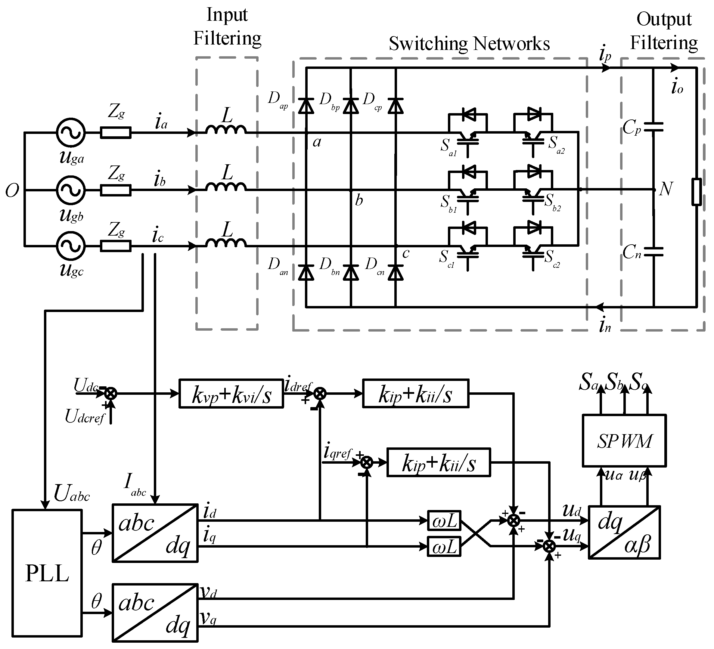
The system block diagram of the Vienna rectifier is shown in Figure 1. Initially, the topology part is considered, where the AC side is connected to a rectifier inductor (L + R), while the DC-link capacitors (Cp&Cn) are linked to the DC-side circuit.
The small-signal notation “^” is used in the differential equation to establish a small-signal-based HSS model, following the circuit relations described in Figure 1. The small-signal state-space equations of the Vienna rectifier are given in Equation (1), where uk is the AC side voltage and ik is the AC side current (k = a,b,c); uko is the voltage at the switching bridge diode clamp point with respect to the AC supply neutral point O; Ik denotes the three-phase current steady-state value; and Ro is the load resistor of the output side:
We define the switching function as follows:
Using logic switches Sip, Sio, Sin (i = a, b, c) to represent the three positions of the equivalent switches of each phase (Sio is the switching signal of the switching tube), Equations (3)–(5) can be obtained from the state averaging method and the circuit relationship:
where ukN is the voltage from the AC input of the rectifier to the neutral point N on the output side; uNO is is the voltage from the neutral of the output side to the neutral of the AC power supply; and Uc1 and Uc2 indicate the steady-state values of the upper and lower bus capacitor voltages on the DC side, respectively.
According to ucp = ucn = 0.5 udc, the small signal of uao, ubo, and uco in Equation (1) can be given as in Equation (6):
where Si0 is the steady-state values of defined switching functions (i = a, b, c) and udc0 is the steady-state value of output voltage.
According to the LTP theory, converting the state-space equations to the frequency domain yields the equations shown in Equation (7) [28]:
where X(ω,t), Y(ω,t), and U(ω,t) represent state variables, output variables, and input variables, respectively, while denotes the convolution operation.
All time-domain signals x(t) can be expressed as in Equation (8), where xk represents the Fourier coefficient, ω0 is the angular frequency, and k denotes the harmonic order:
This can be written as a matrix expression, as shown in Equation (9):
where
The state-space equations in the time domain can be converted to the frequency-domain form as in Equation (12):
where A, B, C, and D are Toeplitz matrices composed of the complex Fourier coefficients of A(t), B(t), C(t), D(t), and X, Y, U are column matrices obtained by arranging from −h to h times.
Thus, Equation (1) can be converted to the HSS equation shown in Equation (13):
where
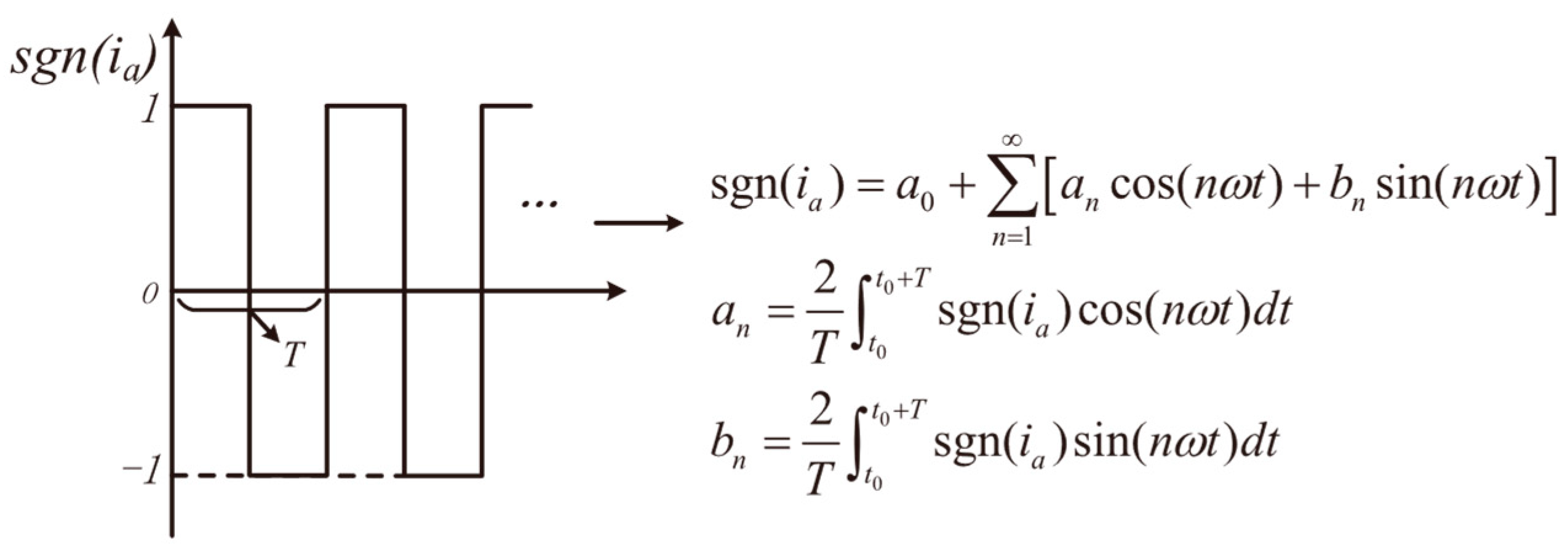
The capital letters in Equations (13)–(17) are the harmonic coefficient components ranging from […−h…−1,0,1…h…] derived from the Fourier series. Furthermore, I denotes the identity matrix, with Zm being a zero matrix of the same size as the considered harmonics and N representing a diagonal matrix. Γ[⊙] denotes the Toeplitz matrix of the corresponding element. To obtain the Toeplitz matrix of the switching function, it is necessary to perform a Fourier series expansion:
where sgn(ik) is the sign function of the input current, given as follows:
Since the sign function of the input current is a periodic rectangular wave, it can be converted into the form of a triangular series summation, as shown in Figure 2, where a0 is the DC components, and an and bn are the coefficients of the sine and cosine terms, respectively.
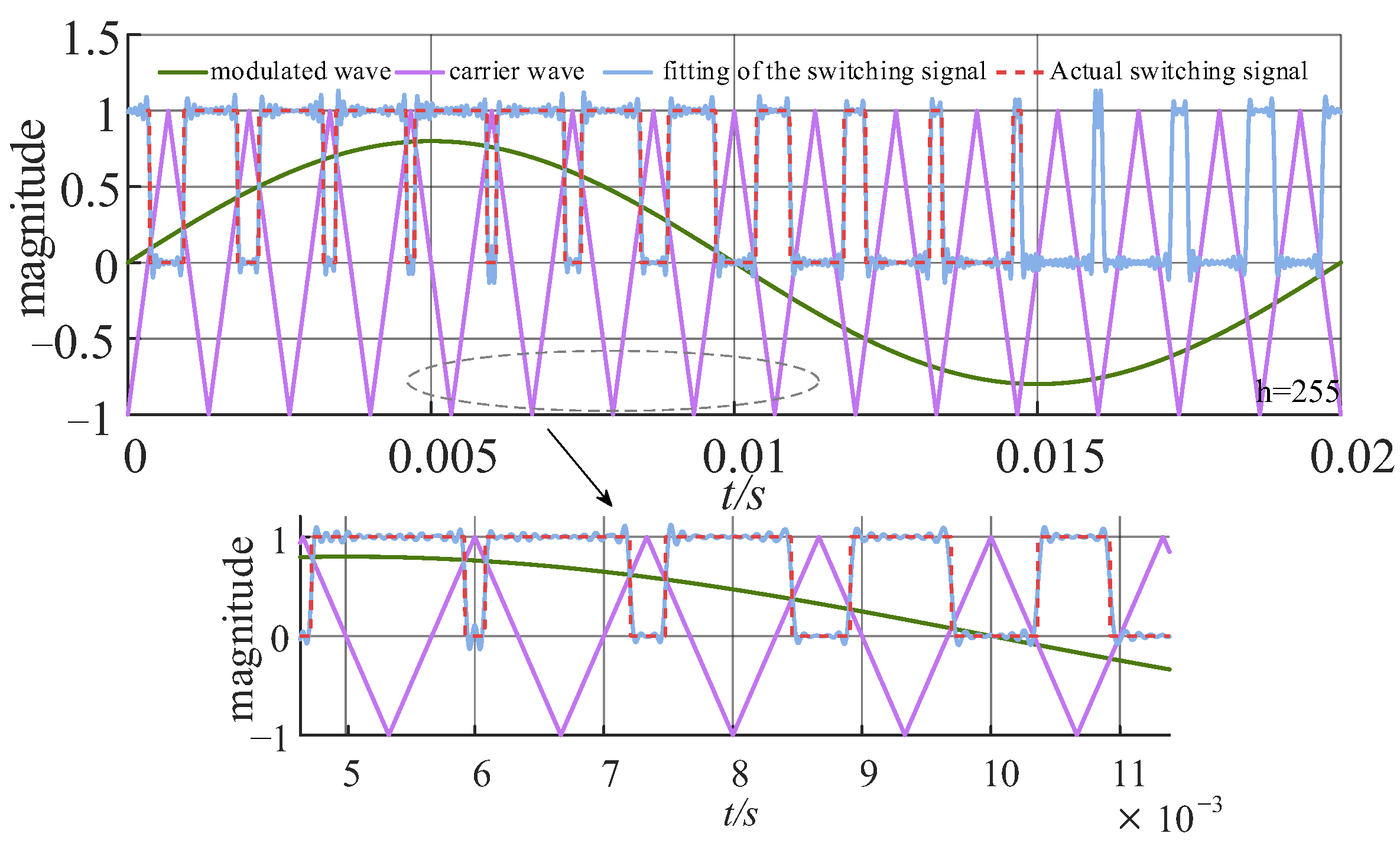
For the switching signal of the switching tube, take phase A as an example. In order to match the switching signal, it is necessary to use the Bessel function. The fitted waveforms obtained by the above method are shown in Figure 3.
From the convolution theorem, it is possible to simplify the product of the Fourier expansions of the two functions to the following equation:
where cn, dm, and hk are the individual Fourier coefficients of the functions f(x), g(x), and h(x), respectively. h(x) = f(x)g(x), and δk,n+m is the Kronecker function.
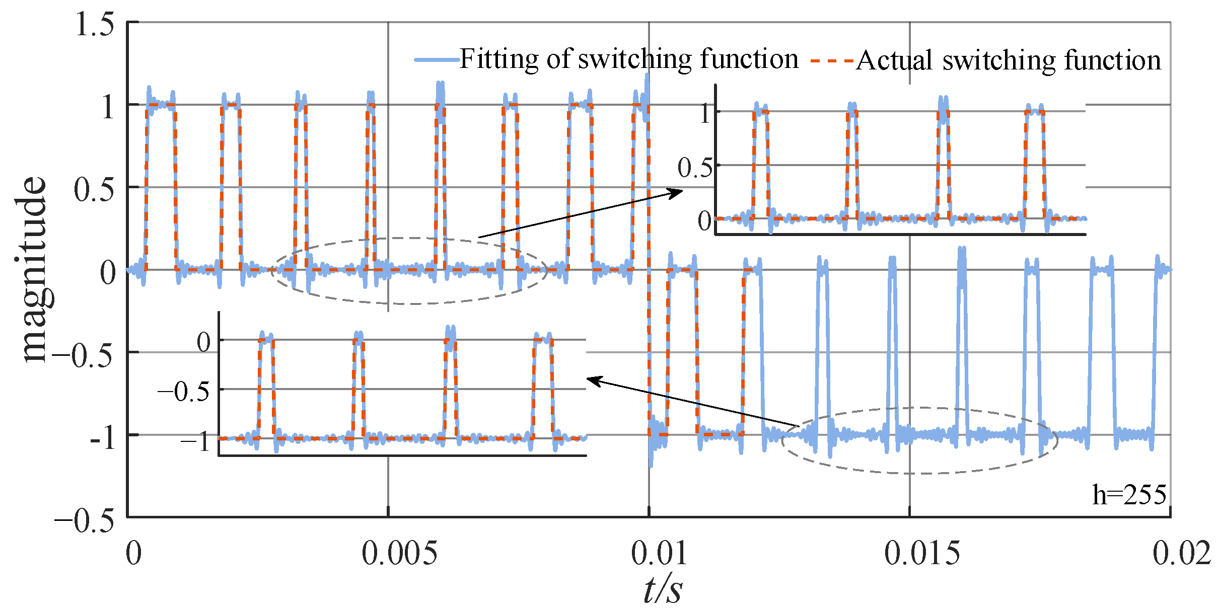
When h = 255, the Sa(t) function fitting, as well as the comparison plot of the actual switching signal, is shown in Figure 4, where the carrier ratio is 15 and the modulation regime is 0.8.
When the system is in a steady state, the s variable will converge to 0, sX = 0. At this time, the harmonic transfer function matrix in a steady state can be obtained as in Equation (21):
2.2. Controller Modeling
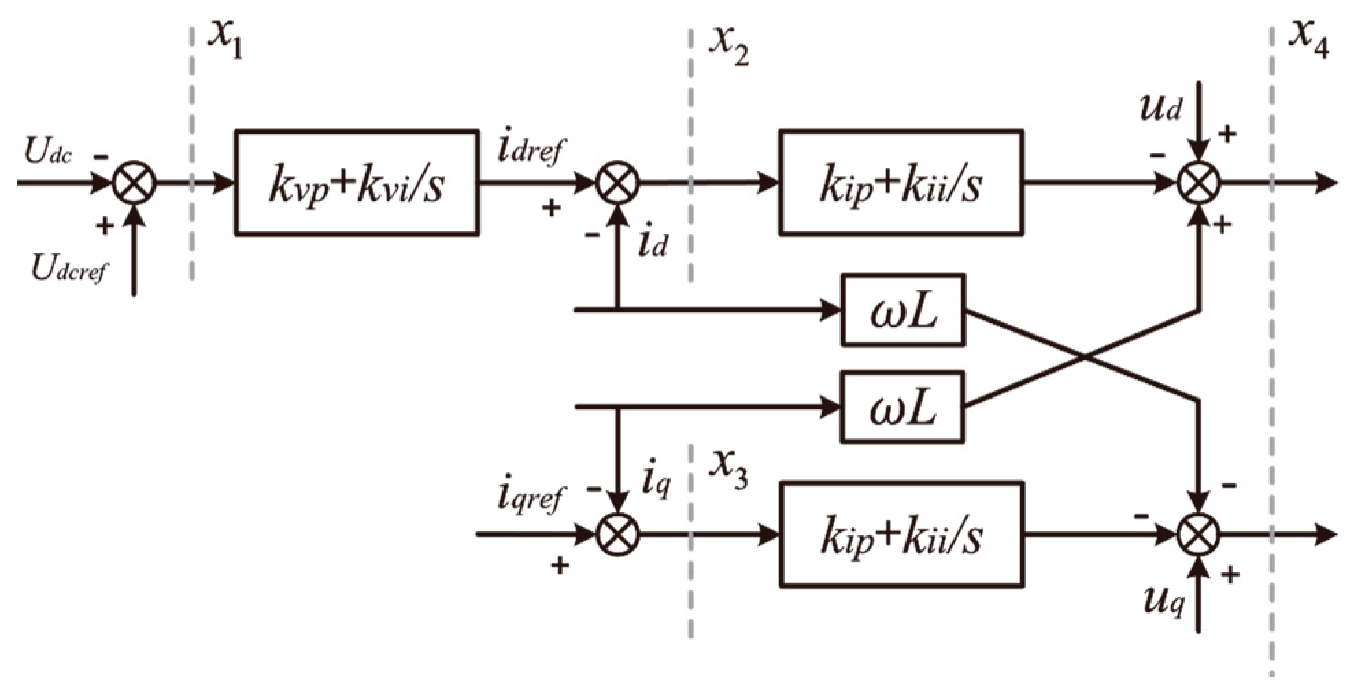
The main control system consists of a voltage outer loop, a current inner loop, a phase-locked loop, and additional components. According to the structure shown in Figure 5, the controller’s modeling involves transforming the time-domain differential equation into a frequency-domain differential equation, as shown in Equation (22):
where x1 to x3 denote the state variables; k1 = kvp, k2 = kvi, k3 = kip, k4 = kii, udc indicate DC-side voltage; and id and iq indicate the dq-axis current.
Additionally, the Park’s transformation in the frequency domain can be represented as given in Equation (23):
where
For the signals x4d and x4q to the abc coordinate system, the Park inverse transform must be applied. This transformation allows for the derivation of the harmonic state-space equations of the control circuit, as given in Equations (24)–(27):
where
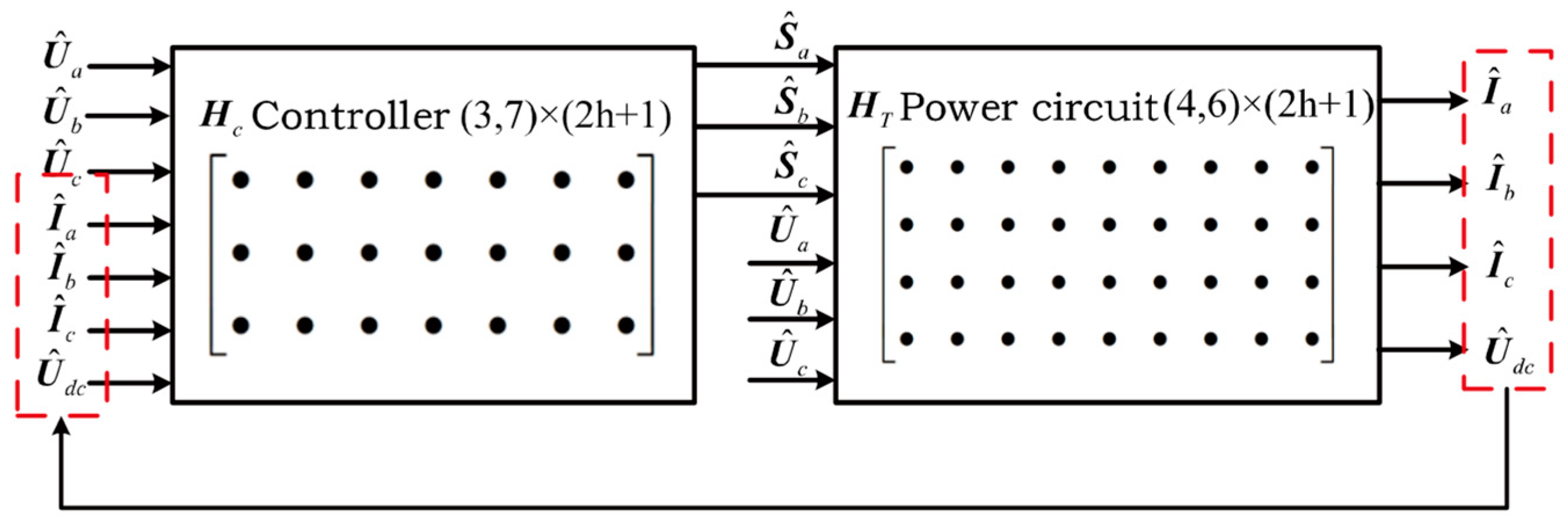
2.3. HSS Model of Vienna Rectifier under Closed-Loop Control
In conclusion, the HSS model of the topology is represented by Equation (13), and the controller HSS model Equation (24) can be connected, as shown in Figure 6.
To obtain the complete HSS small-signal model, the intermediate variable Yc should be eliminated. Thus, the HSS model is given in Equation (32):
where
Note that BT, Bc, and Dc in Af and Bf contain subscripts denoting the submatrices of the original matrix after chunking, where the state quantities Bc1, Bc2, Bc3, Dc1, Dc2, Dc3 are the partition matrices of the corresponding matrices.
Based on the HSS model obtained from the above derivation, Equation (32) under the steady-state solution can be given as Equation (37):
This can be mathematically manipulated to be given as in Equation (38):
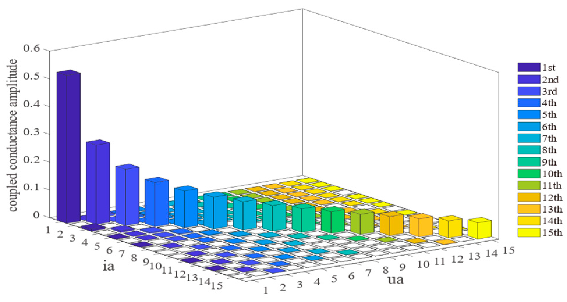
Taking the first sub-matrix Ya in HVienna as an example, it reflects the relationship between the a-phase voltage on the AC side and the a-phase current on the AC side. To analyze the degree of the coupling relationship, it is necessary to convert the coefficients in Ya from complex numbers to real numbers. Each element of the matrix corresponds to both its magnitude and phase angle. When the number of harmonics h is taken as 1, the corresponding matrix of harmonic transfer coefficients is as shown in Equation (39):
where H(m,n) denotes the harmonic coupling coefficient, for example, Ya(m,n), which is expressed as the transfer relationship between the nth input voltage and the mth input current.
It can be seen that the diagonal elements represent the coupling between the same frequencies, called mutual coupling, while the non-diagonal elements indicate the coupling relationship between different frequencies, known as hetero-coupling. Moreover, a larger amplitude of the coupling coefficients indicates a higher degree of coupling.
When the mth harmonic is generated in the input voltage, for example, a-phase voltage, its corresponding Fourier series form is as in Equation (40):
where m represents the mth harmonic; Ua,m is the amplitude of the mth a-phase voltage ua; Ua,(±m) denotes the positive and negative Fourier coefficients of the mth a-phase voltage ua; and θm is the phase angle of the mth a-phase voltage ua.
The relationship between the nth input current ia and the mth input voltage ua expressed in terms of harmonic transfer coefficients is shown in Equation (41):
where
where indicates the harmonic coupling coefficient; Ia,n is the amplitude of the nth a-phase current ia; Ia,(±m) denotes the positive and negative Fourier coefficients of the nth a-phase current ia; and θn is the phase angle of the nth a-phase current ia.
It is important to note that, in practice, there may be coupling relationships for more than just nth-order input voltages for mth-order inputs. These relationships may result from the product of the Fourier coefficients of the input variables and the harmonic transfer coefficients (frequency-domain values) at several different frequencies. When h = 15, the coupled conductance amplitude diagram of the AC-side voltage Ua and current Ia can be obtained as shown in Figure 7.
It can be seen that the same-frequency perturbation of the input quantity ua has a dominant influence on the output quantity ia. Additionally, the coupling amplitude matrix of ua to udc shows that the disturbance frequency of the grid-side voltage ωp mainly affects the ωp ± 50 Hz component of the DC-side voltage.
3. Simulation and Experimental Validation
3.1. Simulation and Experimental Analysis
The HSS model is implemented in MATLAB using an m-file. In the Vienna model, the rectifier-side inductor is L = 2 mH, the capacitor is C = 2000 μF, the DC-side voltage is udc = 800 V, the grid-side voltage is 380 V, the rated power is 15 kW, and the switching frequency is 5 kHz. Additionally, the controller parameters of Vienna are kvp = 0.45, kvi = 75, kip = 24, and kii = 100. These parameters are utilized in the simulation. The experimental parameters are harmonized with the simulation parameters. Adjust the resistance value of the resistor based on the load box to ensure consistency between the experimental and simulation power parameters.
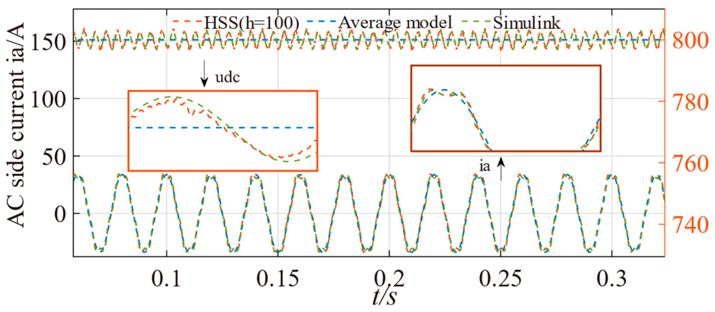
To validate the accuracy of the proposed model, extensive testing is conducted. A 20 V 5th harmonic voltage perturbation is applied to the grid side. The a-phase current waveforms of the AC side under this condition are shown in Figure 8.
From the results in Figure 8, there is a slight difference between the HSS model calculation results and the Simulink results, indicating that the HSS model established in this paper is essentially accurate. When comparing the averaged models, it is evident that the HSS method can accurately consider integer multiples of harmonics within the frequency range. In contrast, the averaging model fails to account for harmonic transmission, rendering it unsuitable for analyzing harmonics in large grids.
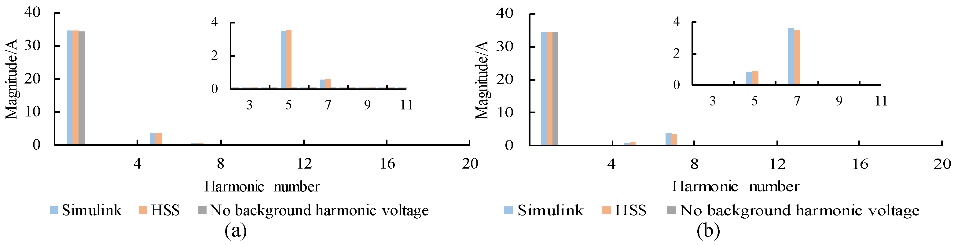
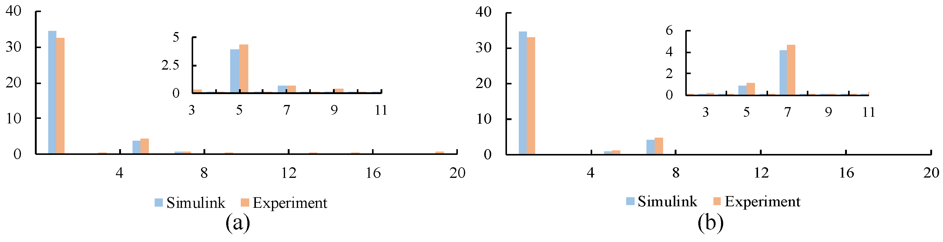
In order to quantitatively analyze the error between the mathematical model and the simulation model, two different working conditions are established to enhance the verification process. The fifth negative sequence voltage and the seventh positive sequence voltage, each with an amplitude of 20 V, are injected into the grid side. The simulation model and the HSS model provide calculated values for the amplitude of each harmonic of the grid-side current, as shown in Figure 9. It can be seen that the amplitude of the harmonic currents calculated by HSS after the introduction of the perturbation is closer to that obtained by Simulink. This demonstrates the advantage of applying HSS to harmonic analysis and highlights the reliability of the modeling.
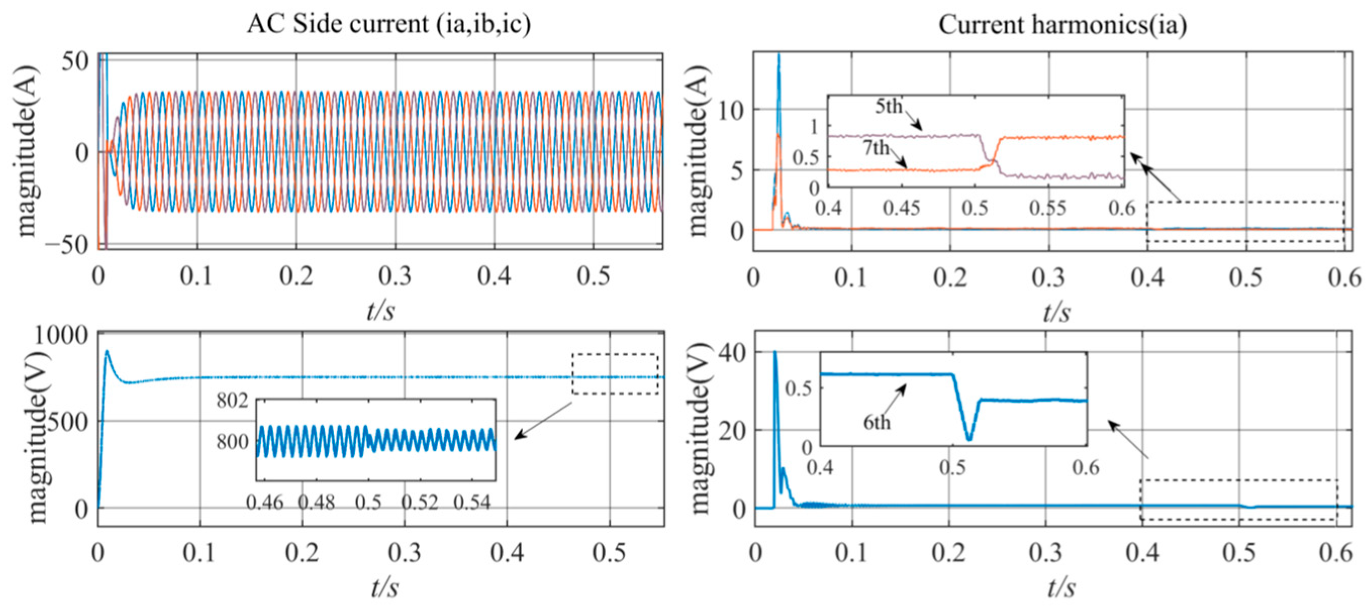
3.2. Harmonic Dynamic Behavior
Figure 10 depicts the dynamic behaviors of harmonics from the HSS model. Initially, the Vienna rectifier operates under “case 1” conditions until 0.5 s, after which the grid voltage harmonics are adjusted to “case 2”. In case 1, there are fifth (25 V) and seventh (5 V) distortions, while, in case 2, there are fifth (12 V) and seventh (25 V) harmonic distortions.
From the results, it can be seen that the magnitude of the 7th harmonic of the current increases as the 7th harmonic in the voltage increases. The harmonics of the DC side also change due to the coupling of the AC side of the rectifier to the DC side through modulation behavior. The DC-side change can be summarized as follows: introducing the fifth negative-sequence voltage perturbation and the seventh positive-sequence voltage perturbation increases the sixth harmonic amplitude of the DC-side voltage.
3.3. Experimental Results
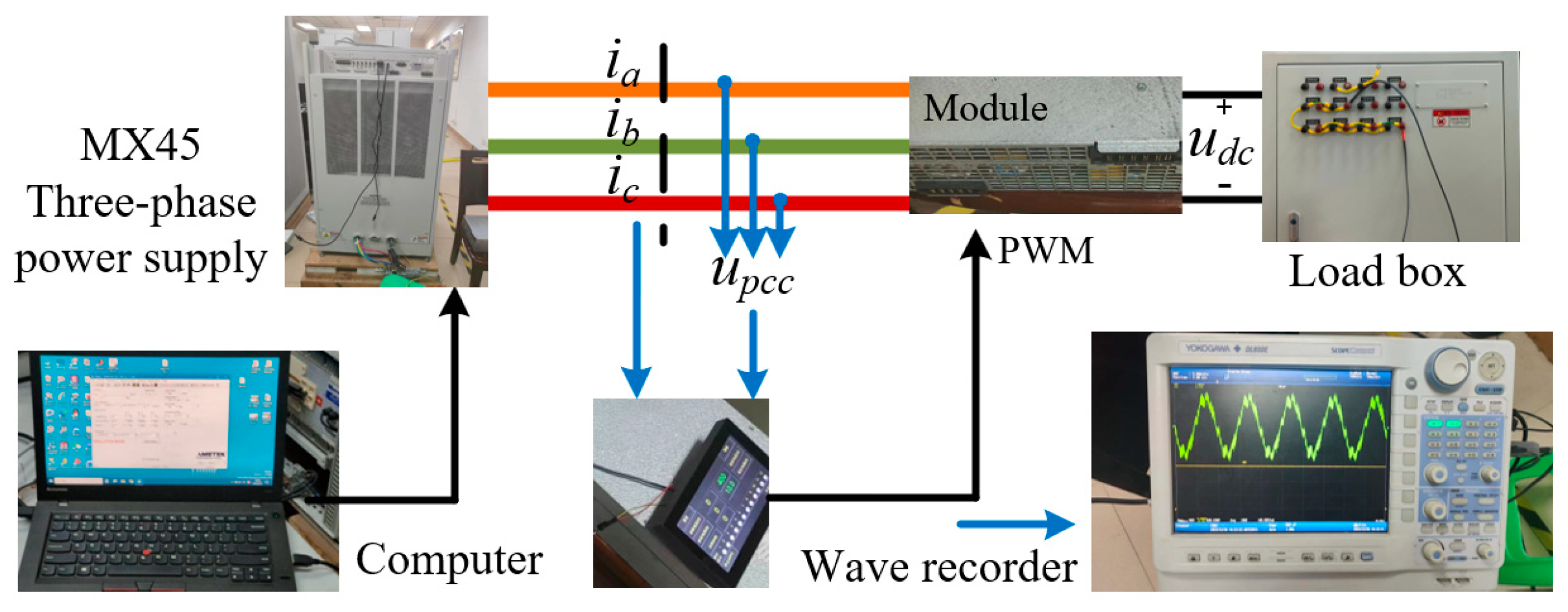
To validate the HSS model from a practical perspective, this paper constructs an experimental platform that includes the Vienna rectifier, as shown in Figure 11. The MX45 three-phase power supply is utilized to power the test module. The module adopts constant DC voltage control, and its output voltage can be set at 200–750 V. The output of this module is connected to a load box comprising several 50 Ω/5 kW resistors connected in series and parallel. The AC-side current is measured using a wave recorder. It is possible to set the fundamental frequency and the harmonic amplitude of the three-phase power supply output by connecting it to the host computer.
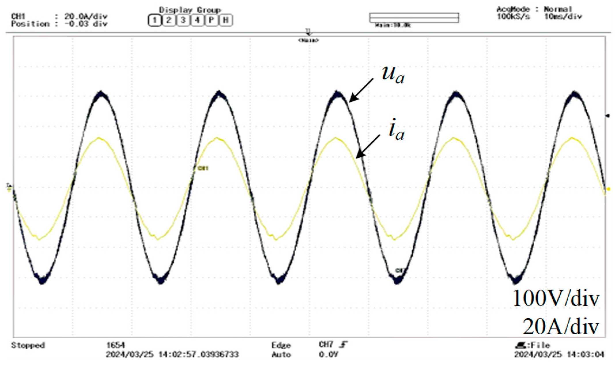
The a-phase voltage and current waveform measured during steady-state operation are shown in Figure 12. It can be seen that the voltage and current remain almost in the same phase, and the power factor is close to 1, ensuring the efficient operation of the system.
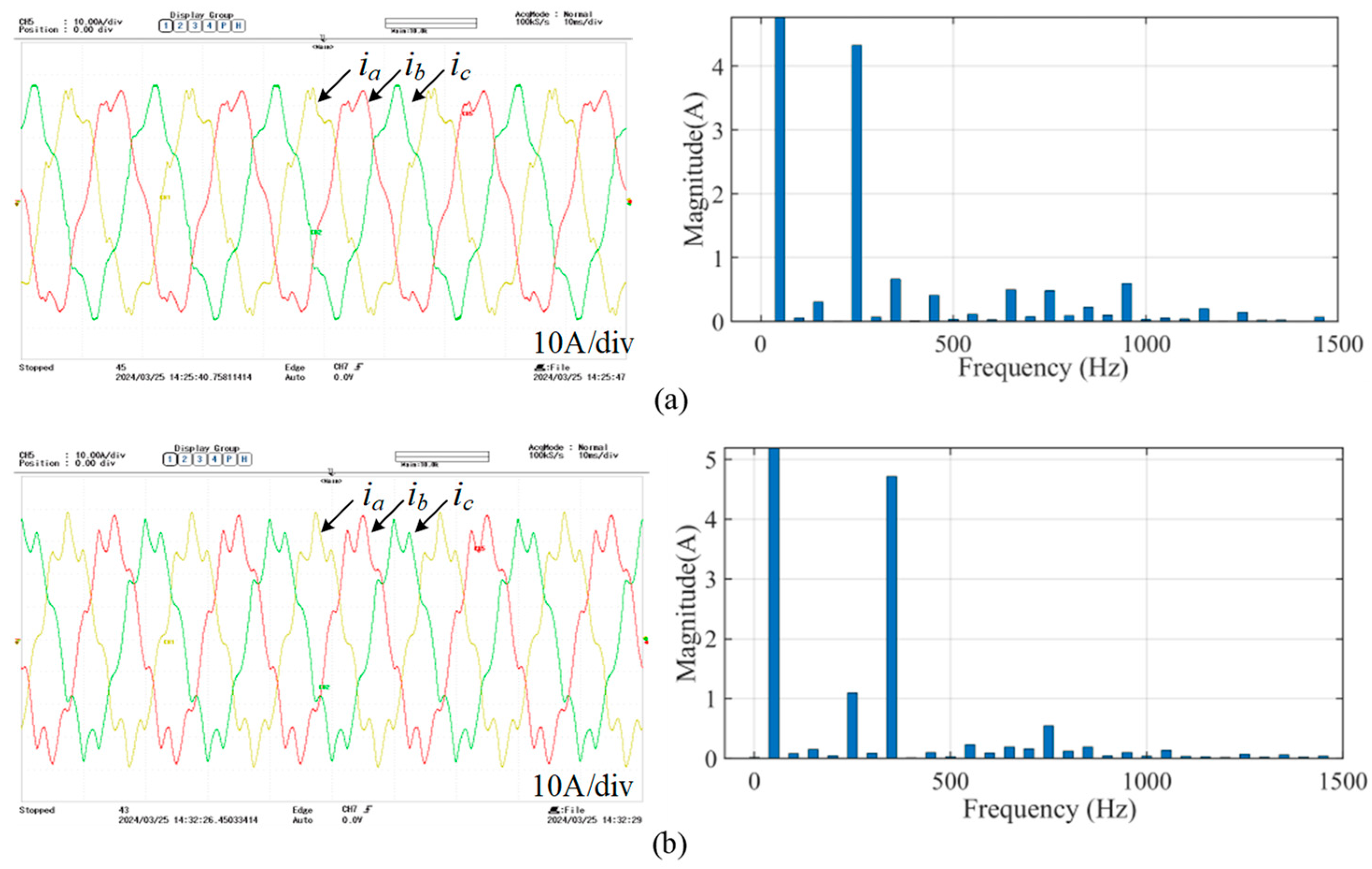
By setting the computer connected to the MX45, the fifth negative-sequence and seventh positive-sequence voltage disturbances, each with an amplitude of 12% of the fundamental waveform amplitude, are injected on the AC side. The three-phase current waveforms at the grid side and their corresponding FFT analysis are shown in Figure 13. It should be noted that the perturbation injection involves simultaneously injecting the three phases with voltages of the same amplitude and frequency. The experimental results show that voltage perturbation primarily causes an increase in the amplitude of AC current at the same frequency. Additionally, it can be observed that the injection of the fifth negative sequence voltage also causes an increase in the amplitude of the seventh harmonic current. Similarly, the injection of the seventh positive sequence voltage causes an increase in the amplitude of the fifth harmonic current. These findings are consistent with the results obtained from the harmonic coupling conductivity map analysis.
In order to further elucidate the findings, the simulation results are compared with the experimental data. The comparison of the amplitude of each harmonic current between the simulation model and the experimental results under the above two specified working conditions is illustrated in Figure 14. It can be observed that, despite a slight deviation between the two results, the consistency of the law can still be reflected to a certain extent. The difference between the two results may be attributed to the idealization of the components in the simulation model, errors in the FFT analysis, and other factors.
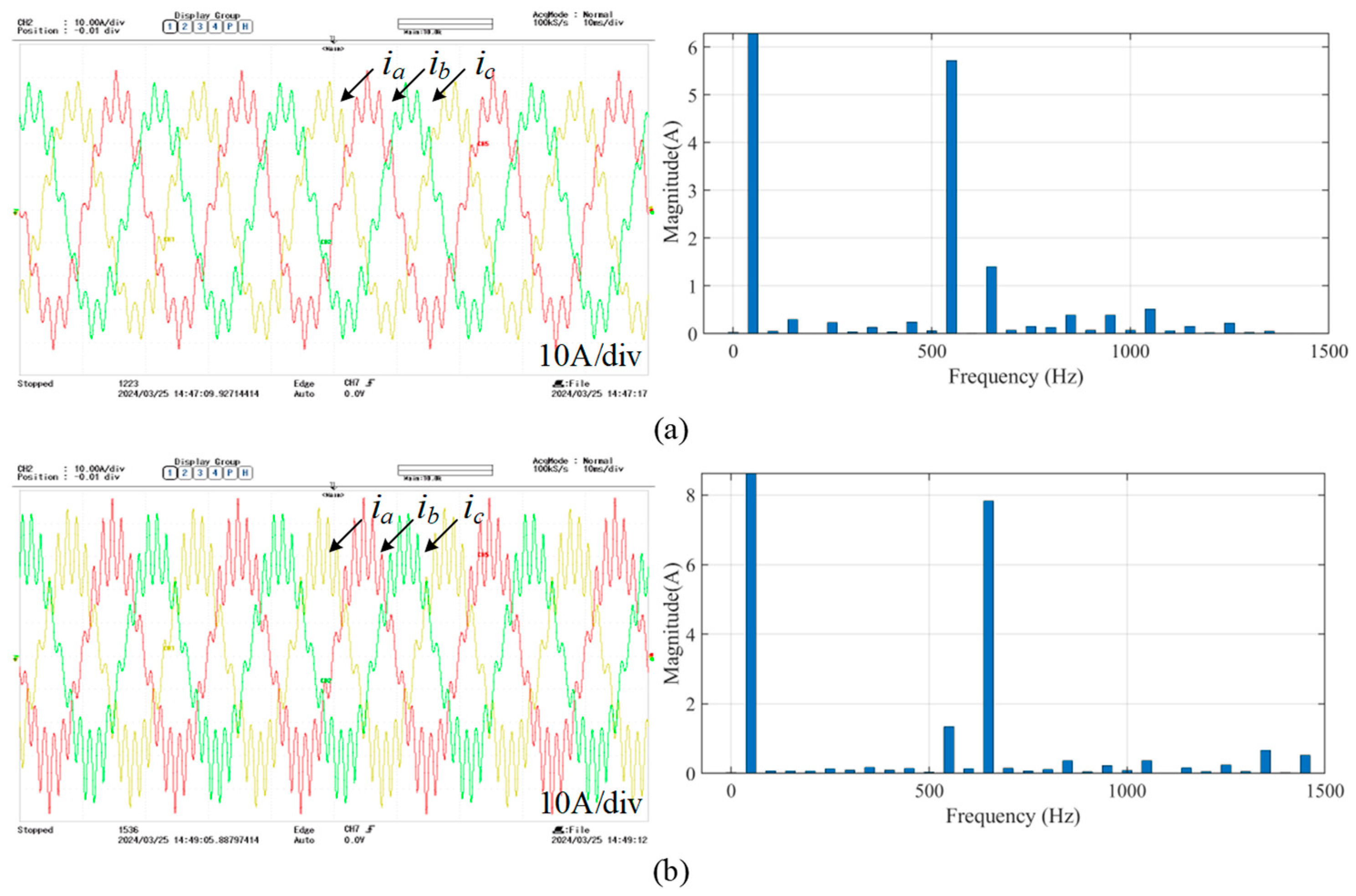
In order to further verify the consistency of the experimental results, two additional sets of tests were conducted to inject 11 negative-sequence voltage disturbances and 13 positive-sequence voltage disturbances. The resulting three-phase current waveforms and the FFT analysis of the corresponding single-phase currents are illustrated in Figure 15.
After injecting the two types of disturbance voltage mentioned above, it is evident that the harmonic amplitude of the grid-side current continues to follow the pattern derived from the analysis. However, it is important to note that, when the amplitude remains constant after injection, the amplitude of the current at the same frequency increases, indicating a higher level of harmonic content.
4. Discussion
Based on the above findings, it is clear that the Vienna rectifier is equally capable of reflecting the frequency-coupling phenomenon. Moreover, according to HSS method, a high-dimensional model can be established from the perspective of the characteristic subharmonics, and then the high-frequency subharmonic steady-state value of the research object is calculated. Compared with other modeling methods, the HSS method can be applied in higher frequency research scenarios. However, as the number of considerations increases, the computational load also increases due to the higher number of matrix orders. Therefore, addressing how to manage degradation has become a crucial issue. Additionally, the HSS method can analyze the harmonic transmission of both the AC and DC sides of the converter, providing advantages in harmonic and stability analysis. Future research on this method will also focus on converters, motors, and electromagnetism.
Compared to other traditional methods, when dealing with time-varying behavior and large network analysis, the HSS approach clearly exhibits distinct advantages. The existing modeling methods handle time-varying variables in diverse manners, where the switching function plays a pivotal role in converter modeling. The switching function serves as the bridging link between the AC and DC sides. However, they simplify this switching function through averaging techniques.
The commonly employed state-space averaging method effectively captures the system’s dynamic response but falls short in analyzing switching frequencies. Conversely, in the dynamic phasor method, although it considers the fundamental frequency component, the switching frequency is ignored. In this paper, the HSS model can be tailored to the desired maximum frequency, accurately describing the system’s dynamic response.
Additionally, as the size and capacity of the converters increase, the difficulty in analyzing them will be further exacerbated. It is crucial to model the frequency coupling between the system and the grid, as well as the transfer characteristics. The state-space averaging method often complicates connecting the DC side of the system to other converters. While models in the dq domain facilitate the analysis of both AC and DC sides, parameter-dependent switching transients can introduce significant deviations, posing additional challenges. Although the dynamic phase method offers improved accuracy in such cases, its descriptive function may overlook the essential coupling components, particularly when coupling is the dominant factor. In such scenarios, the influence of switching transients must be carefully analyzed.
In summary, the HSS method has obvious advantages in the wide-frequency harmonic analysis of a single converter, and the number of harmonic cut-offs considered depends on the context, such as calculation time and range of error. And it can comprehensively consider time-varying behaviors, reveal the frequency coupling behavior of AC and DC sides, and analyze the harmonics of large networks. Moreover, the HSS method can analyze unbalanced systems and has the capability of assessing stability and design controller.
5. Conclusions
This paper delves into the harmonic interaction between the Vienna rectifier and the grid by leveraging HSS modeling. The HSS modeling process, incorporating dual closed-loop control, is introduced to emphasize the distinctions with conventional modeling techniques. Second, to ensure correctness, the established model is benchmarked against time-domain simulation results. Third, the HSS model is employed to examine the harmonic interactions, illustrating the characteristics of harmonics transmission. In addition, the derived model enables one to analyze the frequency-coupling phenomenon. Simulation and experimental results have demonstrated the effectiveness of the model.
Author Contributions
Conceptualization, S.Z. and Y.C.; data curation, S.Z. and B.G.; methodology, S.Z. and J.L.; formal analysis, Y.C. and J.L.; resources, Y.C. and X.D.; writing—review and editing, S.Z., Y.C., J.L. and B.G.; funding acquisition, X.D. All authors have read and agreed to the published version of the manuscript.
Funding
This research was funded by the Key Program of National Natural Science Foundation of China, Grant No. 51937001.
Data Availability Statement
The data are available on request from the corresponding author upon reasonable request.
Conflicts of Interest
The authors declare no conflicts of interest.
References
- Liu, S.; Lin, F.; Fang, X.; Yang, Z.; Zhang, Z. Train Impedance Reshaping Method for Suppressing Harmonic Resonance Caused by Various Harmonic Sources in Trains-Network Systems with Auxiliary Converter of Electrical Locomotive. IEEE Access 2019, 7, 179552–179563. [Google Scholar] [CrossRef]
- Zhao, Z.; Peng, K.; Xian, R.; Zhang, X. Localization of Oscillation Source in DC Distribution Network Based on Power Spectral Density. J. Mod. Power Syst. Clean Energy 2023, 11, 156–167. [Google Scholar] [CrossRef]
- Yu, J.; Lin, X.; Song, D.; Yu, R.; Li, Y.; Su, M. Harmonic Instability and Amplification for Grid-Connected Inverter with Voltage Harmonics Compensation Considering Phase-Locked Loop. IEEE J. Emerg. Sel. Top. Power Electron. 2020, 8, 3944–3959. [Google Scholar] [CrossRef]
- Hou, C.; Zhu, M.; Li, Z.; Li, Y.; Cai, X. Inter Harmonic THD Amplification of Voltage Source Converter: Concept and Case Study. IEEE Trans. Power Electron. 2020, 35, 12651–12656. [Google Scholar] [CrossRef]
- Liu, W.; Zhang, H.; Dong, D.; Liu, W.; Ding, H. Multiharmonic Interaction and Stability Analysis of Two-Stage Double-Input Buck Inverter. IEEE J. Emerg. Sel. Top. Power Electron. 2022, 10, 648–661. [Google Scholar] [CrossRef]
- Todeschini, N.; Balasubramaniam, S.; Igic, P. Time-Domain Modeling of a Distribution System to Predict Harmonic Interaction Between PV Converters. IEEE Trans. Sustain. Energy 2019, 10, 1450–1458. [Google Scholar] [CrossRef]
- Mansouri, A.; Magri, A.; Lajouad, R.; Giri, F.; Adouairi, M.; Bossoufi, B. Nonlinear observer with reduced sensors for WECS involving Vienna rectifiers—Theoretical design and experimental evaluation. Electr. Power Syst. Res. 2023, 225, 109847. [Google Scholar] [CrossRef]
- Mansouri, A.; Magri, A.; Lajouad, R.; Giri, F. Control design and multimode power management of WECS connected to HVDC transmission line through a Vienna rectifier. Int. J. Electr. Power Energy Syst. 2024, 155, 109563. [Google Scholar] [CrossRef]
- Nabinejad, A.; Rajaei, A.; Mardaneh, M. A Systematic Approach to Extract State-Space Averaged Equations and Small-Signal Model of Partial-Power Converters. IEEE J. Emerg. Sel. Top. Power Electron. 2020, 8, 2475–2483. [Google Scholar] [CrossRef]
- Lin, F.; Liu, S.; Yang, Z.; Sun, H. Analysis of nonlinear oscillation of four-quadrant converter based on discrete describing function approach. IEICE Electron. Express 2016, 13, 2016550. [Google Scholar] [CrossRef]
- Daryabak, M.; Filizadeh, S.; Jatskevich, J.; Davoudi, A.; Saeedifard, M.; Sood, V.K.; Martinez, J.A.; Aliprantis, D.; Cano, J.; Mehrizi-Sani, A. Modeling of LCC-HVDC Systems Using Dynamic Phasors. IEEE Trans. Power Deliv. 2014, 29, 1989–1998. [Google Scholar] [CrossRef]
- Yue, X.; Wang, X.; Blaabjerg, F. Review of Small-Signal Modeling Methods Including Frequency-Coupling Dynamics of Power Converters. IEEE Trans. Power Electron. 2018, 34, 3313–3328. [Google Scholar] [CrossRef]
- Wang, H.; Jiang, K.; Shahidehpour, M.; He, B. Reduced-Order State Space Model for Dynamic Phasors in Active Distribution Networks. IEEE Trans. Smart Grid 2020, 11, 1928–1941. [Google Scholar] [CrossRef]
- Chen, D. An improved harmonics detection method based on sliding disrete Fourier transform for three-phase grid-tie inverter system. IEICE Electron. Express 2019, 16, 20181074. [Google Scholar] [CrossRef]
- Zhu, J.; Hu, J.; Wang, S.; Wan, M. Small-Signal Modeling and Analysis of MMC Under Unbalanced Grid Conditions Based on Linear Time-Periodic (LTP) Method. IEEE Trans. Power Deliv. 2021, 36, 205–214. [Google Scholar] [CrossRef]
- Liao, Y.; Wang, X. Small-Signal Modeling of AC Power Electronic Systems: Critical Review and Unified Modeling. IEEE Open J. Power Electron. 2021, 2, 424–439. [Google Scholar] [CrossRef]
- Yang, H.; Just, H.; Eggers, M.; Dieckerhoff, S. Linear Time-Periodic Theory-Based Modeling and Stability Analysis of Voltage-Source Converters. IEEE J. Emerg. Sel. Top. Power Electron. 2021, 9, 3517–3529. [Google Scholar] [CrossRef]
- Zhang, H.; Liu, Z.; Wu, S.; Li, Z. Input Impedance Modeling and Verification of Single-Phase Voltage Source Converters Based on Harmonic Linearization. IEEE Trans. Power Electron. 2019, 34, 8544–8554. [Google Scholar] [CrossRef]
- Sun, J.; Bing, Z.; Karimi, K. Input Impedance Modeling of Multipulse Rectifiers by Harmonic Linearization. IEEE Trans. Power Electron. 2009, 24, 2812–2820. [Google Scholar] [CrossRef]
- Song, Q.; Liu, W.; Li, X.; Rao, H.; Xu, S.; Li, L. A Steady-State Analysis Method for a Modular Multilevel Converter. IEEE Trans. Power Electron. 2013, 28, 3702–3713. [Google Scholar] [CrossRef]
- Wang, K.; Wu, F.; Su, J. Harmonic State-Space Modeling and Closed-Loop Control of Single-Stage High-Frequency Isolated DC–AC Converter. IEEE Trans. Ind. Electron. 2024, 71, 4576–4585. [Google Scholar] [CrossRef]
- Kwon, J.; Wang, X.; Blaabjerg, F.; Bak, C. Frequency-Domain Modeling and Simulation of DC Power Electronic Systems Using Harmonic State Space Method. IEEE Trans. Power Electron. 2017, 32, 1044–1055. [Google Scholar] [CrossRef]
- Kwon, J.; Wang, X.; Blaabjerg, F.; Bak, C.; Sularea, V.; Busca, C. Harmonic Interaction Analysis in a Grid-Connected Converter Using Harmonic State-Space (HSS) Modeling. IEEE Trans. Power Electron. 2017, 32, 6823–6835. [Google Scholar] [CrossRef]
- Motwani, J.K.; Xue, Y.; Nazari, A.; Dong, D.; Cvetkovic, I.; Boroyevich, D. Modeling of Power Electronics Systems and PWM Modulators in Harmonic-State Space. IEEE Open J. Power Electron. 2022, 3, 689–704. [Google Scholar] [CrossRef]
- Gao, G.; Wang, X.; Zhu, T.; Liao, Y.; Tong, J. HSS Modeling and Stability Analysis of Single-Phase PFC Converters. In Proceedings of the 2022 IEEE Applied Power Electronics Conference and Exposition (APEC), Houston, TX, USA, 20–24 March 2022; pp. 1812–1819. [Google Scholar]
- Scapini, R.; Bellinaso, L.; Michels, L. Stability Analysis of AC–DC Full-Bridge Converters With Reduced DC-Link Capacitance. IEEE Trans. Power Electron. 2018, 33, 899–908. [Google Scholar] [CrossRef]
- Wang, X.; Blaabjerg, F. Harmonic Stability in Power Electronic-Based Power Systems: Concept, Modeling, and Analysis. IEEE Trans. Smart Grid 2019, 10, 2858–2870. [Google Scholar] [CrossRef]
- Kwon, J.; Wang, X.; Blaabjerg, F.; Bak, C.; Wood, A.; Watson, N. Harmonic Instability Analysis of a Single-Phase Grid-Connected Converter Using a Harmonic State-Space Modeling Method. IEEE Trans. Ind. Appl. 2016, 52, 4188–4200. [Google Scholar] [CrossRef]
Figure 1.
Block diagram of the Vienna rectifier system.

Figure 2.
Periodic rectangular wave Fourier expansion.

Figure 3.
Switch-signal fitting and theoretical comparison.

Figure 4.
Switch function Sa fitting and theoretical comparison graph.

Figure 5.
Control circuit system diagram.

Figure 6.
Diagram of HSS model and control-circuit HSS model.

Figure 7.
Harmonic coupled admittance amplitude diagram (1st–15th).

Figure 8.
Comparison of AC current waveform under AC voltage disturbance.

Figure 9.
Comparison of simulation model and HSS model. (a) Injection of 5th negative sequence voltage. (b) Injection of 7th positive sequence voltage.
Figure 9.
Comparison of simulation model and HSS model. (a) Injection of 5th negative sequence voltage. (b) Injection of 7th positive sequence voltage.

Figure 10.
Simulation results verify the harmonic interaction.

Figure 11.
Vienna rectifier test platform.

Figure 12.
Grid-side voltage and current waveforms in the same phase.

Figure 13.
AC-side current waveforms with FFT analysis of ia. (a) Injection of 5th negative-sequence voltage of 12% of fundamental frequency amplitude. (b) Injection of 7th positive-sequence voltage of 12% of fundamental frequency amplitude.
Figure 13.
AC-side current waveforms with FFT analysis of ia. (a) Injection of 5th negative-sequence voltage of 12% of fundamental frequency amplitude. (b) Injection of 7th positive-sequence voltage of 12% of fundamental frequency amplitude.

Figure 14.
Comparison of simulation model and experiment. (a) Injection of 5th negative-sequence voltage. (b) Injection of 7th positive-sequence voltage.
Figure 14.
Comparison of simulation model and experiment. (a) Injection of 5th negative-sequence voltage. (b) Injection of 7th positive-sequence voltage.

Figure 15.
AC-side current waveforms with FFT analysis of ia. (a) Injection of 11th negative-sequence voltage of 12% of fundamental frequency amplitude. (b) Injection of 13th positive-sequence voltage of 12% of fundamental frequency amplitude.
Figure 15.
AC-side current waveforms with FFT analysis of ia. (a) Injection of 11th negative-sequence voltage of 12% of fundamental frequency amplitude. (b) Injection of 13th positive-sequence voltage of 12% of fundamental frequency amplitude.

Disclaimer/Publisher’s Note: The statements, opinions and data contained in all publications are solely those of the individual author(s) and contributor(s) and not of MDPI and/or the editor(s). MDPI and/or the editor(s) disclaim responsibility for any injury to people or property resulting from any ideas, methods, instructions or products referred to in the content. |
© 2024 by the authors. Licensee MDPI, Basel, Switzerland. This article is an open access article distributed under the terms and conditions of the Creative Commons Attribution (CC BY) license (https://creativecommons.org/licenses/by/4.0/).
Share and Cite
MDPI and ACS Style
Zhu, S.; Liu, J.; Cao, Y.; Guan, B.; Du, X. Vienna Rectifier Modeling and Harmonic Coupling Analysis Based on Harmonic State-Space. Electronics 2024, 13, 1447. https://doi.org/10.3390/electronics13081447
AMA Style
Zhu S, Liu J, Cao Y, Guan B, Du X. Vienna Rectifier Modeling and Harmonic Coupling Analysis Based on Harmonic State-Space. Electronics. 2024; 13(8):1447. https://doi.org/10.3390/electronics13081447
Chicago/Turabian StyleZhu, Shiqi, Junliang Liu, Yuelong Cao, Bo Guan, and Xiong Du. 2024. "Vienna Rectifier Modeling and Harmonic Coupling Analysis Based on Harmonic State-Space" Electronics 13, no. 8: 1447. https://doi.org/10.3390/electronics13081447
Note that from the first issue of 2016, this journal uses article numbers instead of page numbers. See further details here.