Synchronous Control of High-Speed Train Lift Wing Angle of Attack Drive System Based on Chaotic Particle Swarm Optimization and Linear Auto-Disturbance Resistant Controller

Abstract

In this study, a control scheme is proposed based on Chaotic Particle Swarm Optimization (CPSO) to enhance the Linear Auto-Disturbance Rejection Controller (LADRC). The focus is on addressing the challenge of high-precision variations in angle-of-attack through dual-motor cooperative control within the lifting wing of a high-speed train. The scheme initiates with the design of a dual-loop structure for LADRC, integrating position and current control. The position loop is further refined. Subsequently, the CPSO algorithm is employed to optimize the parameters of the LADRC controller. Ultimately, the loop is closed by feeding back the position error in the cross-coupled structure to the current loop, thereby achieving high-precision control. The performance of the proposed structure is validated through both Matlab/Simulink simulations and an experimental platform. The experimental results demonstrate that CPSO-LADRC, in comparison to traditional LADRC and Proportion-Integration-Differentiation (PID) control, exhibits an increase in the maximum response time by 3.76 s and 3.3 s, respectively, a reduction in overshoot by 1.12% and 0.8%, as well as a decrease in the maximum synchronization error by 0.45 cm and 1 cm, respectively. These findings validate the effectiveness of the proposed synchronous loop controller method in simplifying computational complexity, enhancing system responsiveness, robustness, and synchronization performance. Additionally, our approach facilitates precise angle-of-attack transformation for the lifting wings of high-speed trains effectively.

1. Introduction

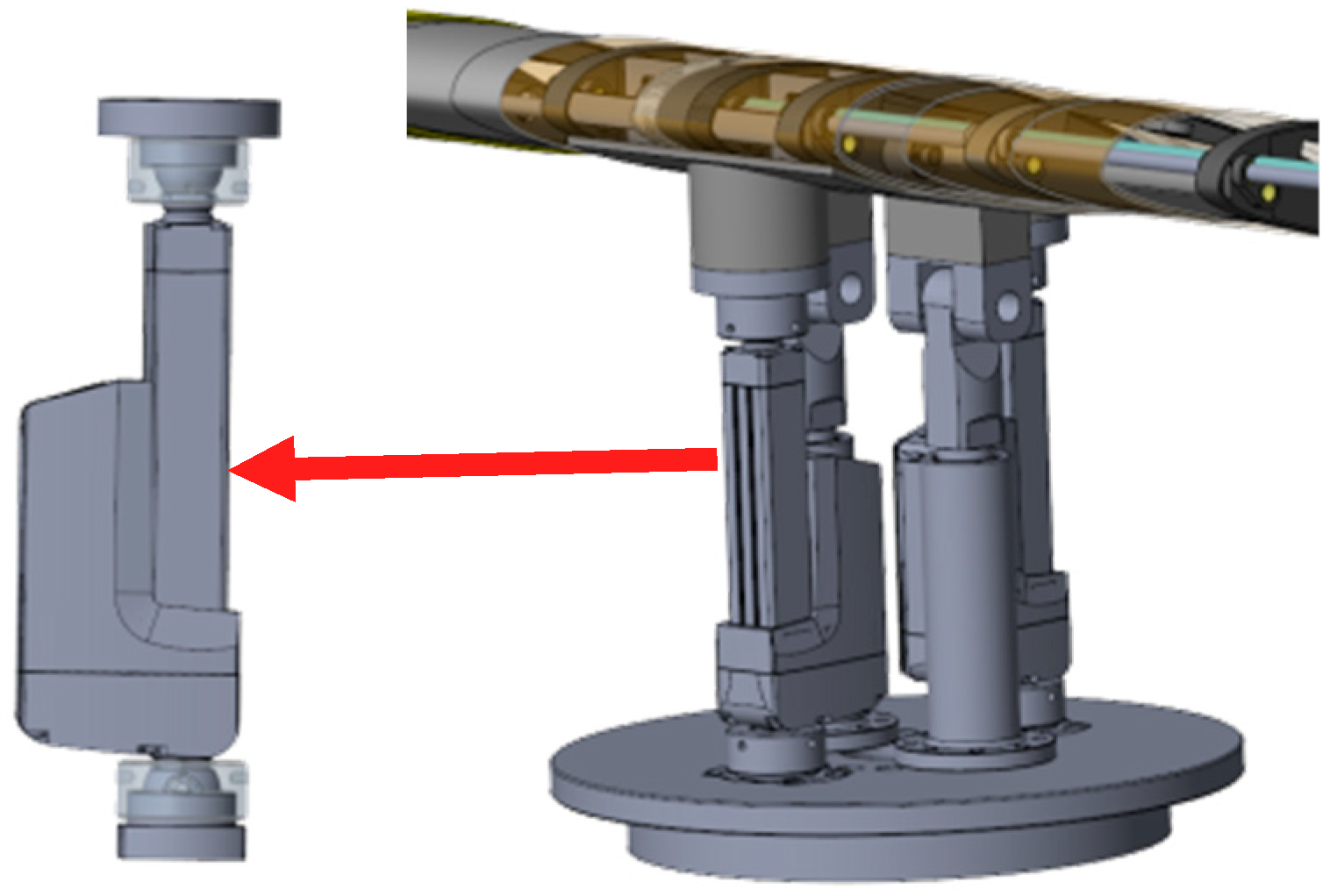
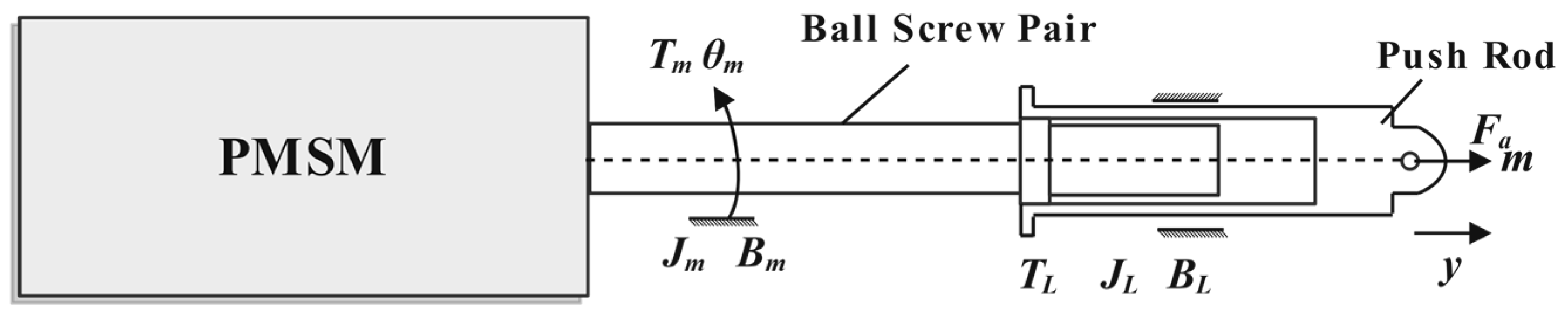
The high-speed train lifting wing represents a novel mechanism designed to achieve train speed reduction and reduce axle weight. This objective is achieved by generating a lift force through precise control of the angle of attack. The structure of the lifting wing is composed of three main components: the angle-of-attack conversion section, the bottom rotation section, and the wing tail contraction section. Notably, the angle of attack conversion section features an electric actuator that is synchronized precisely using two motors.

The precision requirements for angle-of-attack control are stringent due to dynamic load variations on the electric actuator resulting from real-time system changes. Furthermore, the system is subject to numerous internal and external disturbances. Therefore, it is of great importance to achieve precise synchronization between the two motors and possess robust abilities in disturbance rejection.

In the early development of multi-motor synchronous control technology, mechanical linkage-based approaches depended on transmission levers and gear meshing to interconnect multiple motors. However, these systems were plagued by numerous internal and external disturbances, leading to compromised robustness. Along with this, control methods such as master-command control [1], master-slave control, cooperative control, cross-coupling control, and virtual-shaft control [2,3]—well-suited for dual-motor control—have been proposed. Synchronization control methods aim to enhance the stability of the system. However, to address the internal and external perturbation issues in this multi-motor synchronous system, Han [4] proposed the Auto-Disturbance Rejection Control (ADRC) which effectively resolves these challenges. Beyond selecting superior controllers, exploring controller optimization methods is also valuable. In the realm of optimizing conventional controllers, Thor et al. [5] proposed a method for legged robots’ controllers, termed the CPG-RBF network. This method merges the Central Pattern Generator (CPG) with the Radial Basis Function (RBF) network for online adaptive control. Makarem et al. [6] utilized a data-driven approach to iteratively adjust the parameters of the Proportional-Integral-Derivative (PID) controller, thus enhancing its robustness and diminishing its dependency on parameters. Gheisarnejad et al. [7] introduced a controller leveraging deep deterministic policy gradient (DDPG) technology, which minimizes observer estimation errors and enhances the dynamic characteristics of the controller. Regarding the optimization of the ADRC controller, Wang et al. [8] proposed a novel Deep Reinforcement Learning (DRL)-based ADRC to enhance the performance of Permanent Magnet Synchronous Motors (PMSMs). Yang et al. [9] introduced an enhanced velocity compensator into a second-order Linear Auto-Disturbance Rejection Controller (LADRC) deviation coupling control structure, effectively enhancing system accuracy. Tian et al. [10] optimized the extended state observer within the ADRC, suppressing the uncertainty ripple in the current loop and improving the stability of the PMSM system. Nguyen et al. [11] examined the application of a method combining disturbance observer control (DOBC) and ADRC for speed control in PMSMs, improving the stability and robustness of the system. Wang et al. [12] designed a speed controller employing the LADRC with Compensation Function Observer (CFO-LADRC). It addresses the trade-off between dynamic and immune performance. At the same time, it enhances the immunity performance of the system. Liu et al. [13] examined how the error in the velocity loop, when fed back into the ADRC control through a cross-coupling structure. This enhanced the response speed and robustness of the system. Fang et al. [14] proposed an ADRC method with an enhanced extended state observer (ESO) to design a cascade controller for Electromechanical Actuators (EMA) based on PMSM. Wang et al. [15] designed a novel velocity compensator for the deviation coupling structure to compensate for and effectively mitigate self-referencing overruns. This novel compensator greatly enhanced the response and immunity of the system under high-frequency noise conditions. Zhang et al. [16] considered that motor parameters vary with temperature during the synchronous operation of multiple motors. They applied a model reference adaptive algorithm to adjust ADRC parameters online, thereby improving the synchronous control performance of speed in the system. He et al. [17] developed a ring-coupled structure. This structure uses a self-resistant compensator for current compensation in motors. Its purpose is to reduce the synchronization error in a multi-motor system. Abdalla et al. [18] employed Particle Swarm Optimization (PSO) to self-optimize the ADRC parameters and reduce the coupling between these parameters. Yin et al. [19] introduced the ant colony algorithm. This algorithm aims for self-seeking optimization of the ADRC parameters. They proved this approach results in a more robust ADRC controller than the conventional ADRC. Wang et al. [20] introduced artificial intelligence algorithms into the parameter optimization process of the ADRC. They constructed a DRL parameter optimization model. This model automatically optimizes and adjusts the parameters of the controller in various application scenarios.

This paper centers on controlling the angle-of-attack conversion device in the lifting wing.The main contributions are summarized as follows:

(a) The ADRC involves designing nonlinear control laws and optimizing parameters, resulting in a more complex controller design [8,9,10,11]. Although the parameter tuning process of LADRC is relatively straightforward, its linear structure results in poor control performance under nonlinear conditions [12]. Consequently, addressing the complex disturbance issues and high-precision control requirements, the structure of LADRC has been optimized to enhance control performance under nonlinear conditions.

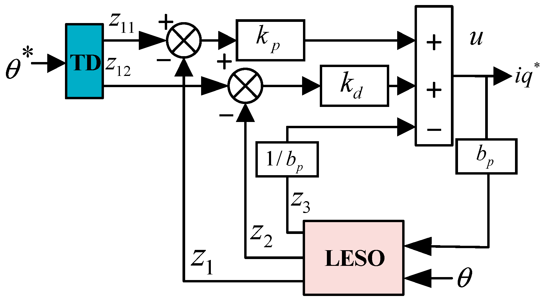
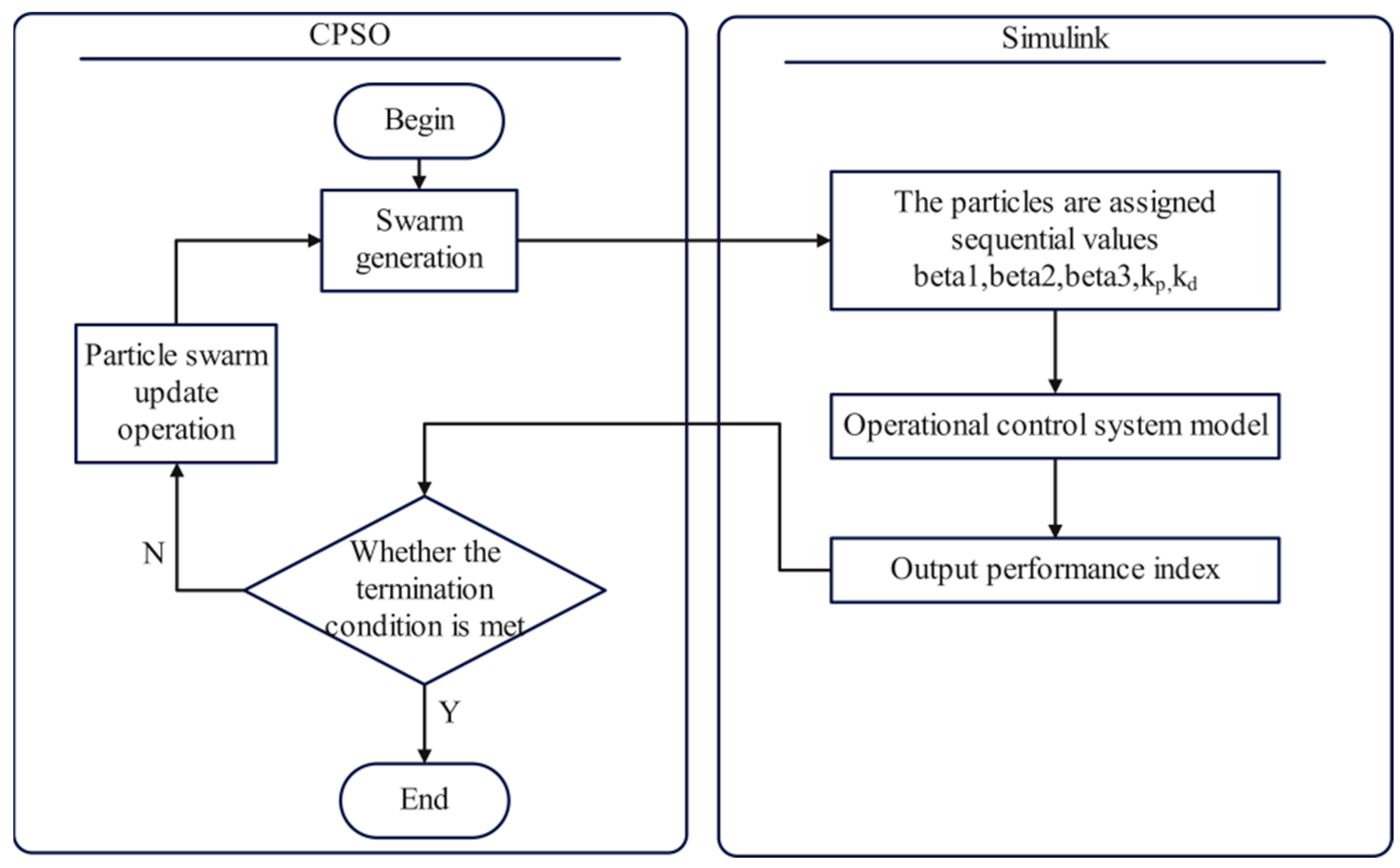
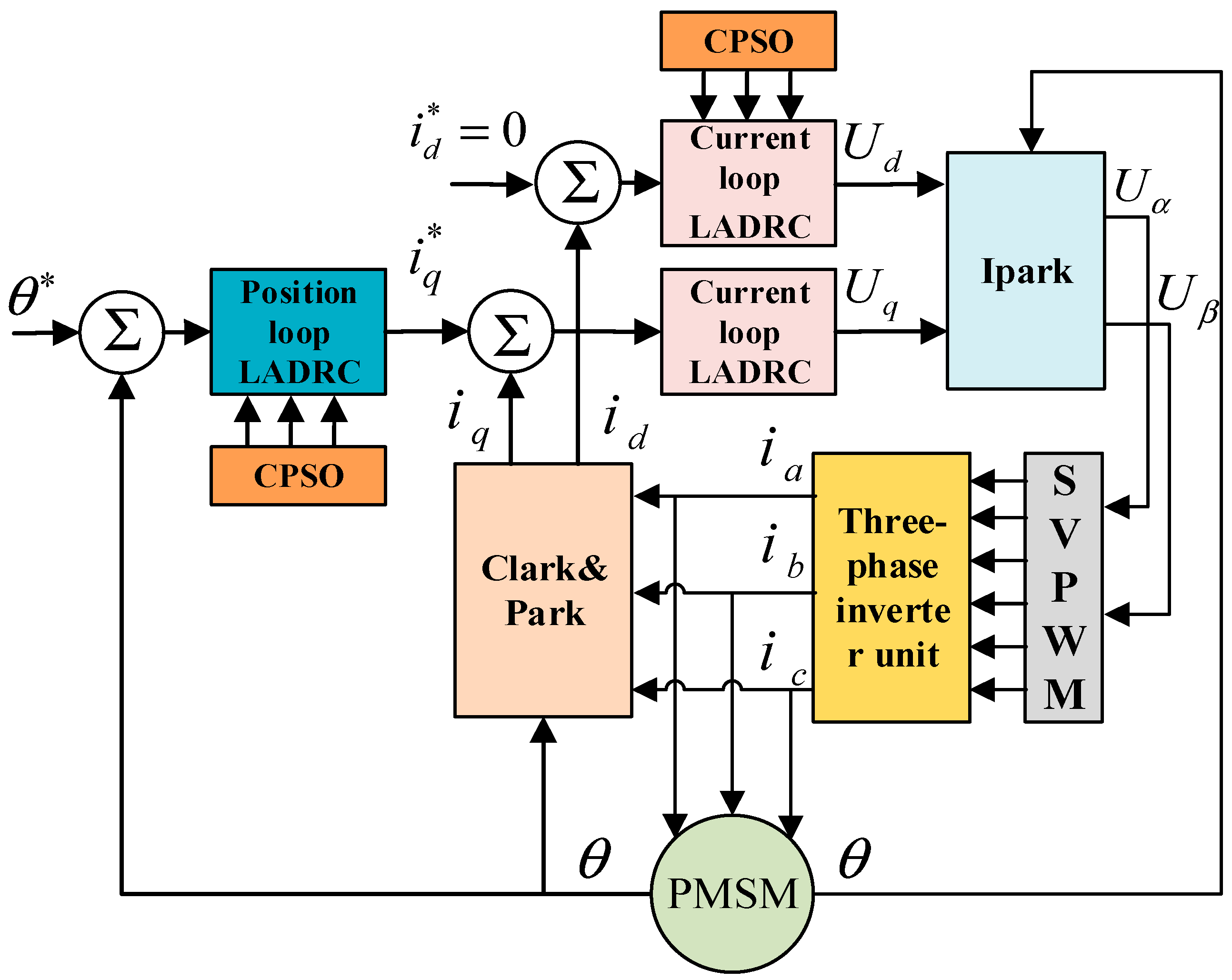
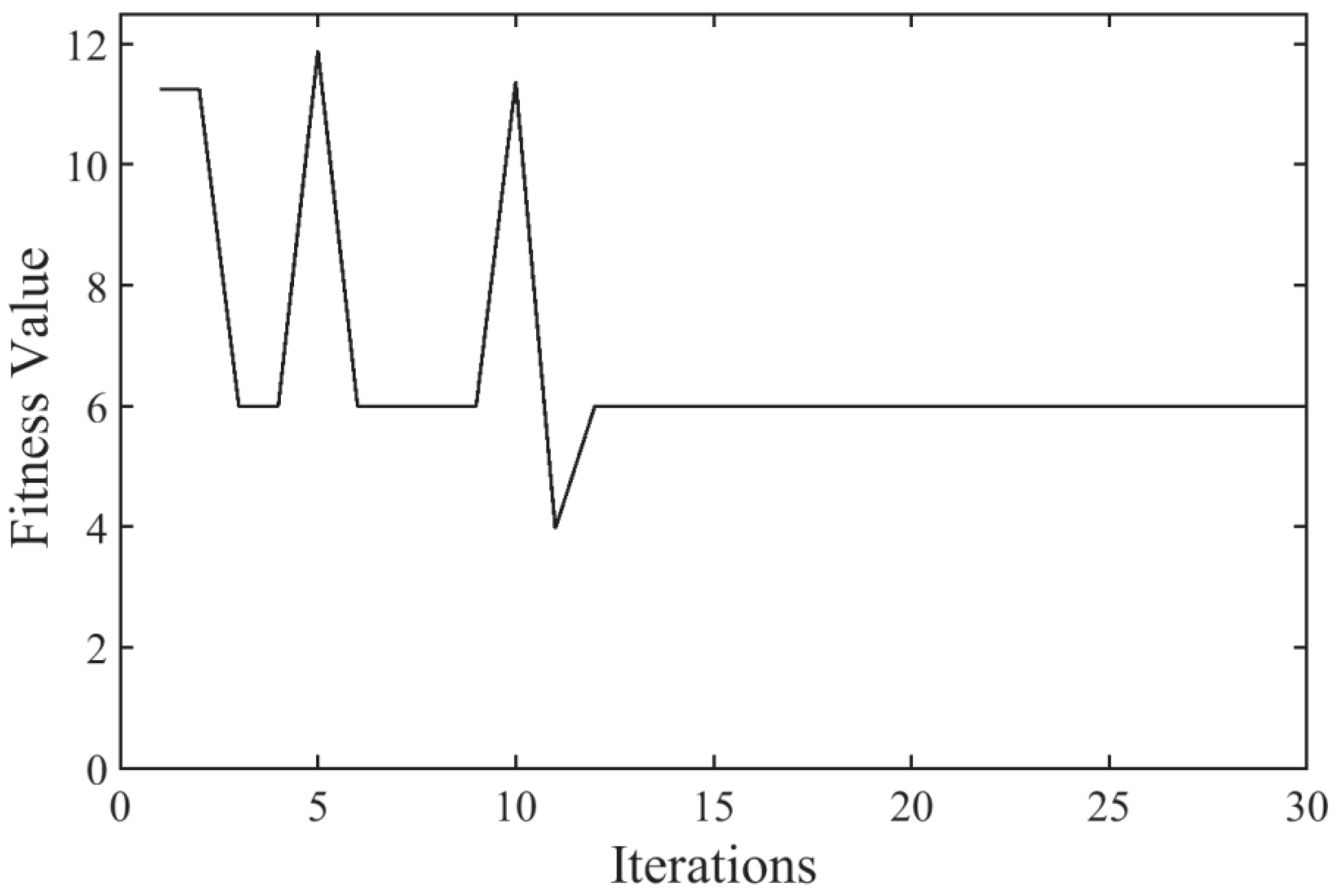
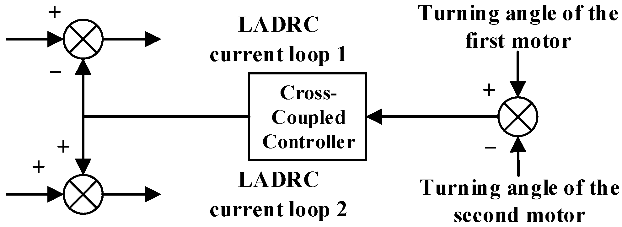
(b) The parameters of the ADRC system are optimized by using the Chaotic Particle Swarm Optimization (CPSO) algorithm. Subsequently, a cross-coupling structure is integrated into the improved LADRC double-loop position control of the servo motor. This structure feeds back the position error to the current loop, thereby enhancing the immunity and response speed of the system. Furthermore, this method effectively addresses the challenge of synchronous control, achieving seamless angle-of-attack conversion.

2. Design of the Lifting Wing Angle of Attack Conversion Device

The angle-of-attack conversion component in the lifting wing is crucial for determining the wing’s angle of attack. This component achieves synchronized reverse movements through the use of motor-driven electric actuators. The structural configuration is illustrated in Figure 1. For precise synchronization, both motors must rotate at identical angles simultaneously, driving the electric actuator to ascend or descend. The input angle of attack of the system guides the calculation for the required height adjustment (rise or fall) of the two electric actuators. Subsequently, the two motors perform forward or reverse rotations at specific angles, effectively controlling the ascent or descent of the electric actuator. Operational schematic diagrams are presented in Figure 2 and Figure 3.

among them:

$$\begin{array}{c}∆h_1=∆h_2\\ ∆h_1=\frac{d·tan\theta }{2}\end{array}$$

(1)

where $∆h_1$, $∆h_2$ are the distance that the two motorized actuators need to be raised/landed, respectively. d is the distance between the two actuators. $\theta$ is the given angle of attack of the system. The lift/landing distance of the motorized actuator is determined by inputting the angle of attack $\theta$, which is subsequently transmitted to the motors through the reducer to obtain arcs $∆{\theta }_1$, $∆{\theta }_2$ rotationally driven by the two motors. These arcs are ultimately utilized as position inputs for precise motor position control.

3. Control System Modeling

3.1. Permanent Magnet Synchronous Motor Modeling

This system requires precise angle-of-attack control. PMSM offers several advantages, such as high efficiency, accuracy, rapid response, and cost-effectiveness. Consequently, we employ the PMSM as the drive motor in this study. First, the mathematical model is established for the PMSM as follows:

$$\begin{gathered} L_q \frac{d{i}_d}{dt}=U_d-R_s i_d+L_q{i}_d {\omega }_e \\ {L}_q \frac{d{i}_q}{dt}=U_q -R_s i_q-\left(L_d{i}_d+{\psi }_f\right){\omega }_e \end{gathered}$$

(2)

where $L_d$, $L_q$ is an estimate of the $dq$-axis inductance, $i_d$, $i_q$ is the dq-axis current $U_d$, $U_q$ is the $dq$-axis voltage, $R_s$ is the stator resistance of the motor, ${\psi }_f$ is the permanent magnet chain of the motor rotor, and ${\omega }_e$ is the rotor speed of the motors.

Figure 4 is the Direct Current (DC) model of a permanent magnet synchronous motor:

where $i_q^{\ast }$ is the current input, $G\left(s\right)$ is the current loop controller, for surface-mounted permanent magnet synchronous motors: $L=L_d=L_q, K_t=p_0{\Psi }_f$ is the electromagnetic torque coefficient, $T_L$ is the load torque, B is the viscous damping coefficient, and J is the equivalent total moment of inertia.

The motor control method employed in this study is the position-current double-loop LADRC control, complemented by the CPSO for tuning the control parameters. Compared to traditional three-loop control, this method ensures position control accuracy and integrates the speed and position loops into the LADRC position loop. This integration not only simplifies the adjustment of control parameters but also enhances the immunity and response speed of the system.

3.2. Electric Actuator Modeling

The PMSM-driven ball screw electric actuator is modeled as shown in Figure 5. The load equivalent combined moment of inertia $J_L$ and load equivalent combined torque $T_L$ are:

$$\left\{\begin{array}{l}{J}_L=J_s+m{(\frac{P_h}{2\pi })}^2\\ T_L=\frac{F_a{P}_h}{2\pi \eta }\end{array}\right.$$

(3)

where $J_s$ is the moment of inertia of the balls-crew shaft, and $m$ is the total mass of the drive and load. $F_a$ is the actuator drive, $P_h$ is the lead of the ball-screw, and η is the positive efficiency of the feed ball-screw subassembly.

The relationship between the angular displacement ${\theta }_m$ of the motor rotation and the linear displacement y of its ball screw actuator advance can be described as follows:

$${\theta }_m=y\frac{2\pi }{P_h}$$

(4)

The rotational moment of inertia and viscous damping coefficients of the system are as follows:

$$\left\{\begin{array}{l}{J}_e=J_m+J_L\\ B_e=B_m+B_L\end{array}\right.$$

(5)

where $J_e$ and $B_e$ are the equivalent rotational moment of inertia and the equivalent viscous damping coefficient at the output shaft of the motor, respectively; $J_m$ and $B_m$ are the rotor moment of inertia and viscous damping coefficient of the motor, respectively. $B_L$ is the load equivalent combined viscous damping factor.

The resulting mathematical model of the system is presented as follows:

$$\left\{\begin{array}{l}{T}_m-T_L-B_e{\dot{\theta }}_m=J_e{\ddot{\theta }}_m\\ y=\frac{P_h{\theta }_m}{2\pi }\end{array}\right.$$

(6)

where $T_m$ is the rated torque of the motor, ${\dot{\theta }}_m={\omega }_r$ is the mechanical angular velocity of the motor rotor output, Assuming that ${\omega }_p$ is the motor angular velocity, then ${\omega }_p=p_n{\omega }_r$, where $p_n$ is the number of motor pole pairs.

3.3. Linear Auto-Disturbance Resistive Control

The angle-of-attack-driven system for lift wings is extensively utilized in industrial applications. However, the intricate operational environment and variable loads on the lift wings necessitate a high disturbance rejection capability and operational precision. Frequently, the conventional PID control architecture falls short in terms of dynamic response. Conversely, ADRC provides advantages in analyzing input-output signals and extracting comprehensive disturbance information, which encompasses both internal and external interferences, for effective compensation [21]. However, optimal parameter tuning presents a formidable challenge for controllers designed to counteract self-disturbances. This requires calibrating multiple parameters, yet a systematic method for calibration remains elusive. After an in-depth study of self-control techniques, Gao [22] proposed the LADRC, which demonstrates robustness and adaptability across various systems. Notably, the parameter tuning process is straightforward. The architecture of the system includes two main components: the Linear State Error Feedback (LSEF) control rate and the Linear Expansion State Observer (LESO). The structure of LESO is shown in Figure 6.

For a specific system of controlled objects, the differential equation can typically be formulated as follows:

$$\ddot{y}=-a_1\dot{y}+f_1+b_{0}u$$

(7)

where $u$, $y$, and $f_1$ are the input, output, and disturbance terms of the system, respectively, $a_1$ and $b_0$ are parameters set in the differential equation of the second order system, respectively.

If the total disturbance of the system is defined as follows:

$$f\left(\dot{y},f_1,t\right)=-a_1\dot{y}+f_1$$

(8)

where t is the time

Equation (7) then becomes:

$$\ddot{y}=f\left(\dot{y},f_1,t\right)+b_{0}u$$

(9)

By setting the following state variables $x_1=y$, $x_2=\dot{y}$, $x_3=f\left(\dot{y},f_1,t\right)$, the following continuously expanding state space equation can be obtained:

$$\left\{\begin{array}{l}{\dot{x}}_1=x_2\\ {\dot{x}}_2=x_3+b_{0}u\\ {\dot{x}}_3=\dot{f}\left(\dot{y},f_1,t\right)\\ y=x_1\end{array}\right.$$

(10)

The LESO corresponding to this system is presented as follows:

$$\left\{\begin{array}{l}{\dot{z}}_1=z_2-{\beta }_1\left(z_1-y\right)\\ {\dot{z}}_2=z_3-{\beta }_2\left(z_1-y\right)+b_0\\ {\dot{z}}_3=-{\beta }_3\left(z_1-y\right)\end{array}\right.$$

(11)

where ${\beta }_1$, ${\beta }_2$, and ${\beta }_3$ are the observer gains.

The system utilizes a linear Proportional-Derivative (PD) controller for the LESF:

$$u_0=k_p\left(R-z_1\right)-k_d{z}_2$$

(12)

where R is the input value, $z_1$ and $z_2$ are the observations of the linearly expanding state observer, and $k_p$ and $k_d$ are the proportional and differential coefficients in the PD controller, respectively.

For the dual-loop control of this system, design the current loop and position loop controllers based on the structure mentioned above.

3.3.1. Current Loop Controller Design

This paper utilizes the $q$-axis current as an example for designing the linear active disturbance rejection controller for the current loop, as it represents the torque current component. The $d$-axis current controller can be designed in reference to the $q$-axis. The differential equations for the $q$-axis current loop are as follows:

$$\frac{d{i}_q}{dt}=-\frac{R_s}{L_q}{i}_q+\frac{1}{L_q}{u}_q-\frac{{\omega }_e{\psi }_f}{L_q}$$

(13)

The first-order LADRC for the current loop is designed based on the above equation. Referring to the structure of Equation (7), the given equation can be rewritten as follows:

$$\frac{d{i}_q}{dt}=f_c+b_c{u}_q$$

(14)

where, $b_c=1/L_q$, $f_c$ is the total current loop perturbation as shown in the following equation:

$$f_c=-\frac{R_s}{L_q}{i}_q+\frac{1}{L_q}{u}_q-\frac{{\omega }_s{\psi }_f}{L_q}-b_c{u}_q$$

(15)

The second-order LESO for the current loop is designed to observe the total current loop perturbation $f_c$ using the following equations:

$$\left\{\begin{array}{l}{\dot{z}}_{iq}={\beta }_{i1}\left(i_q-z_{iq}\right)+z_{fc}+b_c{u}_q\\ {\dot{z}}_{fc}={\beta }_{i2}\left(i_q-z_{iq}\right)\end{array}\right.$$

(16)

where ${\dot{z}}_{iq}$ and ${\dot{z}}_{fc}$ are the values of $i_q$ and $f_c$ observations, respectively, and ${\beta }_1$ and ${\beta }_2$ are the observer gain coefficients.

Based on the pole configuration method in LADRC [22,23], the characteristic equation for the current loop can be derived from the provided equation:

$${\lambda }_0\left(s\right)=s^2+{\beta }_{1}s+{\beta }_2={\left(s+{\omega }_0\right)}^2$$

(17)

where ${\omega }_0$ is the bandwidth of the observer.

The gain of the LESO for the current loop can be determined as follows:

$$\left\{\begin{array}{l}{\beta }_{i1}=2{\omega }_0\\ {\beta }_{i2}={{\omega }_0}^2\end{array}\right.$$

(18)

The LESF is designed using a proportional (P) control structure with the gain $k_p={\omega }_c$. The expressions for the control law $u_0$ and the control quantity $u_q$ are provided below:

$$\left\{\begin{array}{l}{u}_0=k_{ip}\left(i_q^{\ast }-z_1\right)\\ u_q=\frac{u_0-z_2}{b_c}\end{array}\right.$$

(19)

The overall structure of the current loop is depicted in Figure 7.

3.3.2. Position Loop Controller Design

Based on the DC model of PMSM, the dynamic equations of the system can be expressed as follows:

$$\frac{d^2\theta }{d{t}^2}=-\frac{B}{J}\frac{d\theta }{dt}+\frac{K_t}{J}{i}_q-\frac{T_L}{J}$$

(20)

where B is the viscous damping coefficient, J is the equivalent total moment of inertia, $T_L$ is the load torque, $K_t$ is the electromagnetic torque coefficient, and $K_t=p_0{\psi }_f$, $p_0$ is the number of poles of the motor.

Based on the provided equation, the design of a second-order linear active disturbance rejection controller for the position loop can be formulated. Considering the structure of Equation (7) and approximating the transfer function of the current closed-loop control system as 1, the equality $i_q^{\ast }$ = $i_q$ can be derived, thus allowing for the transformation of Equation (20) as:

$$\frac{d^2\theta }{d{t}^2}=f_p+b_p{i}_q^{\ast }$$

(21)

where $b_p=K_t/J$, $f_p$ is the total position loop perturbation as shown in the following equation:

$$f_p=-\frac{B}{J}\frac{d\theta }{dt}+\frac{K_t}{J} i_q-\frac{T_L}{J}-b_p i_q^{\ast }$$

(22)

The total disturbance is observed by designing the third-order LESO for the position loop with the following equations:

$$\left\{\begin{array}{l}{\dot{z}}_{\theta }={\beta }_{s1}\left(\theta -z_{\theta }\right)+z_n\\ {\dot{z}}_n={\beta }_{s2}\left(\theta -z_{\theta }\right)+z_{fp}+b_p{i}_q^{\ast }\\ {\dot{z}}_{fp}={\beta }_{s3}\left(\theta -z_{\theta }\right)\end{array}\right.$$

(23)

where, ${\dot{z}}_{\theta }$, ${\dot{z}}_n$ and ${\dot{z}}_{fp}$ are the observed values of motor angle $\theta$, motor speed n, and total disturbance $f_p$, respectively. ${\beta }_1$, ${\beta }_2$ and ${\beta }_3$ are all observer gain coefficients.

Utilizing the pole configuration method within the framework of LADRC, the characteristic equation for the position loop can be derived from the provided equation, as shown in the expression below:

$${\lambda }_0\left(s\right)=s^3+{\beta }_1{s}^2+{\beta }_{2}s+{\beta }_3={\left(s+{\omega }_0\right)}^3$$

(24)

The observer gain in the linear ESO for the position loop can be obtained as follows:

$$\left\{\begin{array}{c}{\beta }_1=3{\omega }_0\\ {\beta }_2=3{\omega }_0^2\\ {\beta }_3={\omega }_0^3\end{array}\right.$$

(25)

In this context, observations indicate that the conventional LADRC structure leads to excessively long system regulation times. To address this limitation, considering that the $fal$ function in the conventional ADRC structure exhibits superior control efficiency and immunity to disturbances [24,25], an enhanced approach is proposed. To improve input signal tracking and system performance, the Tracking Differentiator (TD) is introduced. The TD is combined with the LESO and the LSEF, with the aim of enhancing system immunity and control performance. The structure of the $fal$ function is represented by the following equation:

$$fal\left(e,\alpha ,\delta \right)=\left\{\begin{array}{l}{\left|e\right|}^{\alpha }sign\left(e\right),\left|e\right|>\delta \\ \\ \frac{e}{{\delta }^{1-\alpha }},\left|e\right|\le \delta \end{array}\right.$$

(26)

The tuning session of the TD parameter is designed as follows:

$$\left\{\begin{array}{l}{\dot{z}}_{11}=\left(z_{11}-{\theta }^{\ast }\right)\cdot k_0\cdot fal\left(e,\alpha ,\delta \right)\\ z_{12}={\dot{z}}_{11}\end{array}\right.$$

(27)

where ${\theta }^{\ast }$ is a given angle and $z_{11}$ is the angle input after parameter adjustment.

The LESF is designed after the session of parameter calibration, as shown in the following equation:

$$\left\{\begin{array}{l}{u}_0=k_{sp}\left(z_{11}-z_1\right)+k_{sd}\left(z_{12}-z_2\right)\\ \\ i{q}^{\ast }=u_0-\frac{z_3}{b_P}\end{array}\right.$$

(28)

where $u_0$ is the control rate and $i{q}^{\ast }$ is the amount of control.

The overall form of PD control is used, which is generally taken as $k_p={\omega }_c^2$ and $k_d=2{\omega }_c\xi$ according to the linear ADRC principle. In $k_d$, $\xi$ is the system damping ratio, ${\omega }_c$ is the bandwidth of the controller.

The comparative simulation of the conventional LADRC and the improved structure is illustrated in Figure 8, while their control performance is presented in

Table 1. Comparison of control indicators.

	Traditional LADRC	Improved LADRC
First response time in place $t_1$/s	0.58	0.21
Second response time in place $t_2$/s	1.24	0.74
First overshoot in place ${\delta }_1$/%	0.01	0.03
Second overshoot in place ${\delta }_2$/%	0.02	0.04
First steady-state error in place ${\mathsf{\Delta }}_1$/cm	0.02	0.01
Second steady-state error in place ${\mathsf{\Delta }}_2$/cm	0.01	0.01

.

In comparison, the response time of the improved LADRC is significantly faster, with the first and second settling times reduced by 0.27 s and 0.50 s, respectively. Additionally, the amount of overshoot and steady-state error between each other is essentially comparable.

The overall structure of the position loop is depicted in Figure 9.

3.3.3. ADRC Parameter Tuning

The performance of the double-loop structure hinges entirely on the efficacy of the self-immunity controller. Therefore, meticulous selection of the second-order ADRC parameters is crucial, as their values directly influence the control performance. This, in turn, determines the overall control effectiveness of the double-loop system. Hence, parameter optimization and careful tuning of the ADRC controller are essential. Taking the self-resistant controller designed by this system as an example, the parameters to be optimized include {${\beta }_l$,${\beta }_2,{\beta }_3$} in LESO and {$k_P,k_d$} in LESF. Only when these parameter values are reasonable and well-coordinated as a whole would the ADRC function be optimal. The interaction among these parameters is intricate, and they exhibit a wide distribution range. The traditional manual calibration method, which relies predominantly on the expertise of designers and iterative experimentation, is both challenging and laborious. Under such conditions, achieving the optimal control effect can be exceedingly challenging.

The PSO algorithm represents a widely studied and applied parallel optimization technique in science and engineering. Renowned for its simplicity, rapid search speed, and efficacy in yielding favorable optimization outcomes, PSO frequently serves as the method of choice for parameter tuning in ADRC systems. In this paper, we introduce the CPSO as an optimized iteration of the PSO algorithm. The CPSO is specifically employed to optimize and fine-tune the critical parameters of the self-resistant position controller. This approach enables a swift exploration of optimal controller parameter values and effectively tackles the challenge of parameter tuning.

3.4. Chaotic Particle Swarm Optimization Algorithm

3.4.1. Particle Swarm Optimization Algorithm Fundamentals

The PSO algorithm begins by initializing a group of particles in the feasible solution space. Each particle represents a set of potential solutions and holds position, velocity, and fitness values. These particles explore the solution space to find an optimal solution. Throughout the iterative optimization process, each particle updates its position by following two poles: the individual best pole (Pbest) and the group best pole (Gbest).

Assuming a D-dimensional search space, the population $X=\left(X_1,X_2,\dots X_n\right)$ comprises n particles, where the ith particle is represented by the vector $X_i={\left(x_{i1},x_{i2},\cdots x_{iD}\right)}^T$, which denotes its position in the search space and a potential solution to the problem. The velocity of the ith particle is $v_i={\left(V_j,V_{i2},\dots V_{ij}\right)}^T$, its optimal position is $P_i={\left(P_{i1},P_{i2},\dots P_{iD}\right)}^T$, and the population extreme value is $P_g={\left(P_{g1},P_{g2},\dots P_{gD}\right)}^T$. The equations for updating the velocity and position of the particle are represented as follows:

$$V_{id}^{k+1}=\omega V_{id}^k+c_1{r}_1\left(P_{id}^k-X_{id}^k\right)+c_2{r}_2\left(P_{gd}^k-X_{id}^k\right)$$

(29)

$$X_{id}^{k+1}=X_{id}^k+V_{id}^{k+1}$$

(30)

where $\omega$ is the inertia weight; $d=1,2,\cdots ,D$; $i=1,2,\cdots ,n$; k is the number of current iterations;${\nu }_{id}$ is the velocity of the particle; $c_1$ and $c_2$ are non-negative constants called acceleration factors; $r_1$ and $r_2$ are distributed in [0–1] numbers. In order to prevent blind search of the particle, it is generally recommended to limit its position and velocity to a certain interval [−$X_{max},X_{max}],\left[-V_{max},V_{max}\right]$.

3.4.2. Improvement of the Algorithm

The CPSO algorithm introduces chaos into the optimization variables to enhance the search process. This is achieved by mapping the traversal range of chaotic motion to the range of values in the optimization variables [26]. The algorithm then explores the cooperation and competition between particles, incorporating small chaotic perturbations, and updating the particle velocity and position until it finds the optimal solution [27].

The execution process involves randomly generating the initial population, initiating a random search, and generating new individuals utilizing the PSO algorithm. If the historical optimal particle position Gbest remains unchanged or changes very little, the algorithm conducts a chaotic search within a certain range centered on Gbest. The optimal solution obtained through this chaotic search is subsequently considered the new Gbest, continuing the solving process.

The optimization problem’s objective function is defined as follows:

$$minf\left(x_1,x_2,\cdots ,x_n\right)s.t.a_i\le x_1\le b_i$$

(31)

The CPSO algorithm follows the subsequent steps:

Step 1: During initialization, set the maximum allowable number of iterations or the adaptation error limit and configure parameters related to the CPSO algorithm, such as inertia weights and learning factors.

Step 2: Chaotic initialization of particle positions and velocities.

(1)

Randomly generate an n-dimensional vector, $z_1=\left(z_{11},z_{12},\cdots ,z_{1n}\right)$, according to Equation (32) to get N vectors $z_1,z_2,\cdots ,z_N$.

$$z_{n+1}=\mu z_n\left(1-z_n\right) n=0,1,2,\cdots$$

(32)

When µ is set to µ = 4 in Equation (32), the system becomes completely chaotic.

(2)

Ensure each component of Z is within the range of values for the corresponding variable.

(3)

Calculate the fitness value of the particle swarm and then select the M solutions with the better performance as the initial solutions from the N initial populations. Additionally, M initial velocities are randomly generated.

Step 3: Revise the individual polar value Pbest according to each particle’s fitness value.

Step 4: Revise the global polar value Gbest according to each particle’s fitness value.

Step 5: Update the velocity and position of the particles using Equations (29) and (30).

Step 6: Chaotic optimization of the optimal location $P_i={\left(P_{i1},P_{i2},\cdots P_{iD}\right)}^T$. Map $P_i$ to the definition domain of the Logistic equation [0,1], $z_i=\left(p_{gi}-a_i\right)/\left(b_i-a_i\right),\left(i=1,2,\cdots D\right)$, then, iteratively generate the sequence of chaotic variables $z_i^{\left(m\right)}\left(m=1,2,\dots \right)$ by using the Logistic equation. The generated sequence of chaotic variables should be returned to the original solution space through the inverse mapping $p_{gi}^{\left(m\right)}=a_i+\left(b_i-a_i\right)z_i^{\left(m\right)}$, resulting in:

$$P_g^{\left(m\right)}=\left(P_{i1}^{\left(m\right)},P_{i2}^{\left(m\right)},\cdots ,P_{iD}^{\left(m\right)}\right),\left(m=1,2,\cdots \right)$$

(33)

3.4.3. Optimization of ADRC Parameters Using CPSO

The optimization problem for ADRC involves determining an appropriate set of parameters {${\beta }_{s1},{\beta }_{s2},{\beta }_{s3},k_{sp},k_{sd}$}, {${\beta }_{i1},{\beta }_{i2},k_{ip}$} to optimize the performance metrics. Commonly used error performance metrics include the Integral of Squared Error (ISE), the Integral of Absolute Error (IAE), the Integral of Time-weighted Absolute Error (ITAE), and the Integral of Squared Time-weighted Error (ISTE). In this case, the Integral of Time-weighted Absolute Error (ITAE) metric has been selected, which is defined as:

$$J={{\displaystyle \int }}_0^{\infty }t\left|e\left(t\right)\right|dt$$

(34)

The application process of the algorithm employs the chaotic particle swarm algorithm to optimize the design of classical second-order position ADRC parameters. The current loop optimization process remains unchanged and is depicted in Figure 10.

The application process of the algorithm utilizes the chaotic particle swarm algorithm to optimize the design of classical second-order position ADRC parameters. The realization process is depicted in Figure 10, and the optimization procedure for the current loop aligns with that of.

The overall control structure of the system after CPSO optimization is shown in Figure 11.

3.4.4. Simulation Study of CPSO Algorithm Optimization

The CPSO algorithm optimally tunes the eight parameters of the ADRC controller and compares the results with those obtained by the conventional linear self-immunity parameter tuning method. The ADRC position controller has eight parameters that need to be tuned and optimized. These include the {${\beta }_{s1},{\beta }_{s2},{\beta }_{s3},k_{sp},k_{sd}$} of the position loop and the {${\beta }_{i1},{\beta }_{i2},k_{ip}$} of the current loop. For both algorithms, the total number of the particle population is n = 20, the dimension of the search space is D = 8, and the number of iterations is T = 30. The acceleration factor is ${\mathrm{c}}_1={\mathrm{c}}_2=$2, and the inertia factor is $w=$ 0.6.

Table 2. PMSM parameter.

Parameter Name	Value
DC side voltage ${\mathrm{U}}_{\mathrm{dc}}$/V	24
Rated torque ${\mathrm{T}}_{\mathrm{m}}$/N·m	0.2
Rated Power ${\mathrm{P}}_{\mathrm{N}}$/KW	0.064
Back electromotive force ${\mathrm{K}}_{\mathrm{e}}/(\mathrm{V}/\mathrm{krpm})$	4.3
Rated speed ${\mathrm{n}}_{\mathrm{N}}$/rpm	3000
Stator resistor ${\mathrm{R}}_{\mathrm{s}}$/Ω	0.12
d-axis inductance ${\mathrm{L}}_{\mathrm{d}}$/mH	0.59
q-axis inductance ${\mathrm{L}}_{\mathrm{q}}$/mH	0.59
Permanent magnet chain ${\mathsf{\psi }}_{\mathrm{f}}$/Wb	0.0175
Moment of inertia J/(kg·m2)	0.00019
Polar logarithm P	4

shows the motor parameters.

Optimal controller parameters and performance indicators can be obtained after operation.

Table 3. Parameter tuning results of the LADRC for the two algorithms.

Algorithm	${\mathbf{\beta }}_{\mathbf{s}1}$	${\mathbf{\beta }}_{\mathbf{s}2}$	${\mathbf{\beta }}_{\mathbf{s}3}$	${\mathbf{k}}_{\mathbf{s}\mathbf{p}}$	${\mathbf{k}}_{\mathbf{s}\mathbf{d}}$	${\mathbf{\beta }}_{\mathbf{i}1}$	${\mathbf{\beta }}_{\mathbf{i}2}$	${\mathbf{k}}_{\mathbf{i}\mathbf{p}}$
LADRC	227.79	17,296.09	437,764.16	499.97	51.32	996.24	248,123.53	1794.21
CPSO-LADRC	321.63	14,258.64	512,253.36	587.58	54.34	1254.36	386,543.48	2165.22

provides a comparison between the resulting parameters obtained after operation and the traditional LADRC parameter tuning method.

In Figure 12, the final fitness value obtained from the algorithm optimization is 6.0128. Subsequently, the PMSM position simulation, optimized with CPSO parameters, is compared with the previously mentioned LADRC for signal tracking, as depicted in Figure 13 and Figure 14.

The maximum deviation errors of the two algorithms for tracking sine waves and triangular waves are presented in

Table 4. Maximum deviation error.

	LADRC	CPSO-LADRC
Sine wave	50.3°	1.8°
Triangular wave	98.2°	2.3°

. It can be inferred from these results that the signal tracking performance of CPSO-LADRC significantly outperforms that of the traditionally parameter-rectified LADRC.

In Figure 15, the position setting is identical to that depicted in Figure 8. From Figure 15, it can be observed that the LADRC optimized through CPSO enables reasonable parameter selection. The PMSM controlled by the controller demonstrates a fast response speed, with a first response time of 0.09 s and a second response time of 0.68 s. Furthermore, the overshoot amounts to less than 0.01%, indicating favorable dynamic and static characteristics.

3.5. Cross-Coupling Control of Dual Motors

To attain synchronous operation between the two motors, a cross-coupling control structure was selected due to its high suitability for synchronizing two motors. The fundamental principle of this structure involves compensating for any position or speed differences between the motors in the input of the controller, thereby achieving coupling of the motor angle, speed, or current. This study utilizes a structure designed to compensate for the position differences among the motors within the current loop. The first motor is subjected to positive feedback, whereas the second motor receives negative feedback. Such an arrangement guarantees consistency in the positions of both motors, thereby enabling synchronous operation. The structure is illustrated in Figure 16.

The positions of the two motors need to be synchronized to rotate to the same position initially. Subsequently, upon reaching time $t_0$, motor 1 is to rotate forward by a specified angle ${\theta }_1$, while motor 2 reverses by the same angle ${\theta }_2$, necessitating continued synchronization. In this specific structure, corrections to the cross-coupled controller inputs within the current loop are depicted as follows:

$$\begin{array}{c}\left\{\begin{array}{c}\Delta i{q}_1=\left(\left|x-{\theta }_1\right|-\left|x-{\theta }_2\right|\right)\cdot k_1\\ \Delta i{q}_2=\left(\left|x-{\theta }_1\right|-\left|x-{\theta }_2\right|\right)\cdot k_2\end{array}\right.t<t_0\\ \left\{\begin{array}{c}\Delta i{q}_1=\left(\left|x-{\theta }_1\right|-\left|x-{\theta }_2\right|\right)\cdot k_1\\ \Delta i{q}_2=-\left(\left|x-{\theta }_1\right|-\left|x-{\theta }_2\right|\right)\cdot k_2\end{array}\right.t\ge t_0\end{array}$$

(35)

where $∆i{q}_1$, $∆i{q}_2$ is the correction value of the current loop of the two motors, x is the given value of the position, $k_1$ and $k_2$ are adjustable parameter. Generally, if the parameters of two motors are identical, the settings are as follows: $k_1$ = $k_2$ = $k_0$.

4. Simulation Studies and Experimental Verification

4.1. Simulation Studies

For the aforementioned system, the simulation model is developed on the Matlab/Simulink simulation platform. Two PMSMs featuring identical parameters are chosen to conduct the simulation. The motor parameters are detailed in Table 2.

The ADRC controller parameter settings, both before and after optimization, are depicted in Table 3 in the cross-coupled controller: x = 35,$k_{0 }$= 1. In the PI control structure used as a comparative experiment, the position loop parameters: $k_{p1}$ = 900, $k_{i1}$= 80, the current loop parameters: $k_{p2}$= 100, $k_{p2}$= 80.

To verify the system’s immunity and synchronization performance, experiments were designed as follows: The distance between the two electric actuators was set at d = 150 cm, the height at h = 35 cm, and the angle of attack at $\theta$= 15°. Subsequently, different inputs were administered to the two motors at distinct positions. Initially, the two motors are synchronized to start both under no load and an asymmetric heavy load (with loads of 5 N·m and 30 N·m, respectively), aiming to simultaneously reach a height of h = 35 cm. At $t_0$= 0.6 s, position signals were set for electric actuator 1 and electric actuator 2 at $∆h_1$=$∆h_2$= 10 cm to observe the effects of reverse synchronization. Figure 17, Figure 18, Figure 19, Figure 20, Figure 21 and Figure 22 depict the simulation results.

The figure above demonstrates that CPSO-LADRC exhibits faster response times and reduced overshoots compared to the traditional parameterized LADRC and PI control. Additionally, the synchronization error is rapidly minimized to zero, yielding a more stable system. To further evaluate the effects of these methods on the synchronization performance of the system, a comparison of control parameters for each controller is presented in

Table 5. Comparison of control parameters for each controller.

		PI	LADRC	CPSO-LADRC
No-load	Maximum synchronization error	0.357 cm	0.002 cm	0.008 cm
	Maximum first response time in place	0.522 s	0.480 s	0.081 s
	Maximum second response time in place	0.751 s	0.814 s	0.701 s
	Maximum first overshoot in place	0.481%	0.005%	0.004%
	Maximum second overshoot in place	0.403%	0.006%	0.003%
Asymmetric load	Maximum synchronization error	1.153 cm	0.793 cm	0.482 cm
	Maximum first response time in place	0.535 s	0.471 s	0.073 s
	Maximum second response time in place	0.746 s	0.803 s	0.698 s
	Maximum first overshoot in place	0.486%	0.007%	0.006%
	Maximum second overshoot in place	0.356%	0.005%	0.003%

.

According to Table 5, under no-load conditions, CPSO-LADRC demonstrates a similar maximum steady-state error and maximum overshoot as traditional LADRC, both at relatively low levels. However, it exhibits significant improvement over PI control. At the same time, with respect to response speed, both traditional LADRC and PI control show significant improvements. Under asymmetric load conditions, CPSO-LADRC demonstrates greater improvements in both maximum steady-state error and response speed than the other two algorithms. Maximum overshoot is comparable to that of traditional LADRC but also shows significant improvement over PI control. Furthermore, Figure 22b illustrates that the two actuators rapidly minimize errors under varying load conditions. These parameter comparisons indicate that the LADRC controller optimized by CPSO provides faster response speeds, lower overshoots, enhanced system dynamics, and improved synchronization performance, demonstrating clear optimization effects.

4.2. Experimental Verification

Utilizing the aforementioned design, we have constructed a multi-motor synchronous control experimental platform, as shown in Figure 23. This platform is designed to facilitate position command tracking experiments under varying load conditions. Our primary objective was to validate the effectiveness of the proposed method in enhancing the performance of self-resistant control. The experimental validation was conducted using a double-screw structure without any mechanical coupling. Furthermore, given that saturation and torque ripple are infrequent in this system, attention to these factors can be deemphasized.

The optimized algorithm was uploaded to the STM32 control board using Data Acquisition Processor (DAP). The STM32F407 is interfaced with two drive boards, facilitating parallel control of two motors. The power supply circuit utilizes a common DC bus structure. Notably, the two motors are directly coupled to the lead screw without mechanical coupling, effectively eliminating interference from mechanical coupling effects. The position information of the motor is captured through a 20-bit high-resolution single-turn absolute encoder. Considering the proportional relationship between the position of the electric push rod and the angular displacement of the motor, the encoder-relayed motor position information undergoes positional data processing via the Digital-to-Analog Converter (DAC), facilitated by the STM32, before being displayed on the oscilloscope. The experimental setup is illustrated in Figure 24. The inverter utilizes Insulated-Gate Bipolar Transistors (IGBTs) and functions at a switching frequency of 16 kHz. Comprehensive details of the motor parameters are presented in Table 2.

Similar to the simulations, the experiments were conducted under both no-load conditions and asymmetric large loads (5 N·m and 20 N·m loads, respectively). The remaining parameters and position settings continued to be consistent with those used in the simulations. The experimental results are depicted in Figure 25, Figure 26, Figure 27, Figure 28, Figure 29 and Figure 30. Notably, following CPSO optimization, the system demonstrated improved response speed, stability, and synchronization performance.

Following the completion of the experiment, the comparison of control parameters under both no-load and asymmetric load conditions is presented in

Table 6. Comparisons of control parameters for each controller.

		PI	LADRC	CPSO-LADRC
No-load	Maximum synchronization error	0.36 cm	0.14 cm	0.13 cm
	Maximum first response time in place	5.21 s	4.75 s	1.45 s
	Maximum second response time in place	7.42 s	8.09 s	6.86 s
	Maximum first overshoot in place	0.66%	0.22%	0.29%
	Maximum second overshoot in place	0.51%	0.31%	0.21%
Asymmetric load	Maximum synchronization error	0.72 cm	1.27 cm	0.27 cm
	Maximum first response time in place	5.32 s	4.61 s	1.44 s
	Maximum second response time in place	7.44 s	8.01 s	6.75 s
	Maximum first overshoot in place	1.66%	1.34%	0.54%
	Maximum second overshoot in place	1.29%	0.82%	0.64%

.

Table 6 clearly shows that, under no-load conditions, CPSO-LADRC demonstrates similar maximum steady-state error and maximum overshoot to traditional LADRC, though with slight differences. However, compared to PI control, CPSO-LADRC exhibits significant improvements. Additionally, both traditional LADRC and PI control show marked enhancements in response speed. Under asymmetric load conditions, the CPSO-LADRC algorithm outperforms the other two regarding maximum steady-state error, response speed, and maximum overshoot. This comparative analysis indicates that the CPSO-LADRC achieves faster response speeds and lower overshoots, ensuring robust system dynamics and improved synchronicity. Experimental validation has confirmed these optimization outcomes.

5. Discussion

This paper proposes a LADRC cross-coupled control structure, utilizing CPSO for optimization. The proposed algorithm underwent subsequent application in both simulation and experimentation phases. Following satisfactory simulation outcomes, the experiments yielded results as follows: Compared to traditional LADRC and PID control, CPSO-LADRC exhibited a maximum increase in response time of 3.76 s and 3.3 s, respectively, along with a reduction in overshoot of up to 1.12% and 0.8% and a decrease in maximum synchronization error of up to 0.45 cm and 1 cm, respectively. Furthermore, under diverse load conditions, both push rods rapidly returned to their zero position, thereby validating the effectiveness of the optimization approach.

Although this approach demonstrates potential for engineering applications, it also reveals certain shortcomings that necessitate further improvements:

(1)

A more refined adaptive parameter tuning method. Although CPSO exhibits a significant optimization effect, the exploration of more intelligent parameter tuning methods represents an important area for improvement. For example, integrating neural networks for parameter tuning could potentially enhance performance.

(2)

Enhanced synchronous loop control. While the ADRC has yielded excellent results, our experiments indicate that even under ADRC control, the motor does not completely utilize its dynamic performance potential. Exploring methods to further enhance the motor’s capabilities emerges as a valuable research direction.

While the ADRC has yielded excellent results, our experiments indicate that even with the ADRC control, the motor does not completely utilize its dynamic performance potential. Exploring methods to further enhance the capabilities of the motor is a valuable research direction.

6. Conclusions

This paper explores the dual-motor cooperative control problem in the lifting wing angle-of-attack drive device of high-speed trains. Initially, the LADRC structure was constructed, and a position-current double-loop LADRC control strategy was designed based on this structure. To optimize the system, the CPSO algorithm was proposed for tuning the parameters of the LADRC, yielding an optimized position-loop LADRC controller. Simulation verification has confirmed that the performance of this mechanism surpasses that of the traditional LADRC.

A cross-coupled synchronization control structure has been employed to synchronize the two motors. The position error in the motor’s position loop was then fed back to the current loop. Subsequently, a multi-motor cross-coupled synchronization control strategy, based on the CPSO-optimized LADRC, was designed. The performance of the two motors under two load conditions (no load and asymmetric load) was compared using the improved LADRC and PID control methods. The results indicate that the CPSO-optimized LADRC cross-coupled control structure exhibits rapid response, smoother regulation, reduced system synchronization error, and enhanced overall control system stability.

References

1. Xu, C.; Hu, H.; Yang, R. Series synchronization control of multi-servo motors. Electr. Autom. 2001, 23, 21–22. [Google Scholar]
2. Lorenz, R.D.; Schmidt, P.B. Synchronized motion control for process automation. In Proceedings of the Conference Record of the IEEE Industry Applications Society Annual Meeting, San Diego, CA, USA, 1–5 October 1989; pp. 1693–1698. [Google Scholar]
3. Payette, K. The virtual shaft control algorithm for synchronized motion control. In Proceedings of the 1998 American Control Conference. ACC (IEEE Cat. No.98CH36207), Philadelphia, PA, USA, 26 June 1998; Volume 5, pp. 3008–3012. [Google Scholar]
4. Han, J. From PID technology to “self-disturbance control” technology. Control Eng. 2002, 9, 13–18. [Google Scholar]
5. Thor, M.; Kulvicius, T.; Manoonpong, P. Generic Neural Locomotion Control Framework for Legged Robots. IEEE Trans. Neural. Netw. Learn. Syst. 2021, 32, 4013–4025. [Google Scholar] [CrossRef] [PubMed]
6. Makarem, S.; Delibas, B.; Koc, B. Data-Driven Tuning of PID Controlled Piezoelectric Ultrasonic Motor. Actuators 2021, 10, 148. [Google Scholar] [CrossRef]
7. Gheisarnejad, M.; Farsizadeh, H.; Khooban, M.H. A Novel Nonlinear Deep Reinforcement Learning Controller for DC–DC Power Buck Converters. IEEE Trans. Ind. Electron. 2021, 68, 6849–6858. [Google Scholar] [CrossRef]
8. Wang, Y.; Fang, S.; Hu, J.; Huang, D. A Novel Active Disturbance Rejection Control of PMSM Based on Deep Reinforcement Learning for More Electric Aircraft. IEEE Trans. Energy Convers. 2023, 38, 1461–1470. [Google Scholar] [CrossRef]
9. Yang, S.; Zhang, S.; Liu, Y. Research on multi-motor synchronous control system based on second-order LADRC. Mach. Tool Hydraul. Pressure 2021, 49, 104–106+172. [Google Scholar]
10. Tian, M.; Wang, B.; Yu, Y.; Dong, Q.; Xu, D. Adaptive Active Disturbance Rejection Control for Uncertain Current Ripples Suppression of PMSM Drives. IEEE Trans. Ind. Electron. 2024, 71, 2320–2331. [Google Scholar] [CrossRef]
11. Nguyen, H.V.; Suleimenov, K.; Nguyen, B.H.; Vo-Duy, T.; Ta, M.C.; Do, T.D. Dynamical Delay Unification of Disturbance Observation Techniques for PMSM Drives Control. IEEE/ASME Trans. Mechatron. 2022, 27, 5560–5571. [Google Scholar] [CrossRef]
12. Wang, C.; Yan, J.; Heng, P.; Shan, L.; Zhou, X. Enhanced LADRC for Permanent Magnet Synchronous Motor with Compensation Function Observer. IEEE J. Emerg. Sel. Top. Power Electron. 2023, 11, 3424–3434. [Google Scholar] [CrossRef]
13. Liu, X.; Chen, R.; Bai, S. Automatic disturbance rejection control of permanent magnet synchronous motor based on particle swarm optimization. J. North China Univ. Technol 2021, 43, 97–103. [Google Scholar]
14. Fang, Q.; Zhou, Y.; Ma, S.; Zhang, C.; Wang, Y.; Huangfu, H. Electromechanical Actuator Servo Control Technology Based on Active Disturbance Rejection Control. Electronics 2023, 12, 1934. [Google Scholar] [CrossRef]
15. Wang, X.; Liu, Y.; Zhong, Y.; Gao, J. Based on self-corrected self immunity control A multi-motor cooperative system. Modul. Mach. Tool Autom. Manuf. Tech. 2021, 63, 77–81. [Google Scholar]
16. Zhang, Y.; Guan, Z.; Wang, T.; Du, P.; Meng, Y. Multi-motor synchronous control based on self disturbance resistance control technology. Electr. Autom. 2017, 39, 9–11+68. [Google Scholar]
17. He, Z.; Yu, H. Ring-coupled multiple-motor coordinated sliding mode control based on self-immunity and observer. Micromotor 2021, 54, 48–55. [Google Scholar]
18. Abdalla, M.A.; Yang, G.; Huang, C. Performance comparison active disturbance rejection control tuned by particle swarm optimization technique and gravitational search algorithm based load frequency control. In Proceedings of the 16th IET International Conference on AC and DC Power Transmission (ACDC 2020), Online, 2–3 July 2020; pp. 2128–2134. [Google Scholar]
19. Yin, Z.; Du, C.; Liu, J.; Sun, X.; Zhong, Y. Research on Autodisturbance-Rejection Control of Induction Motors Based on an Ant Colony Optimization Algorithm. IEEE Trans. Ind. Electron. 2018, 65, 3077–3094. [Google Scholar] [CrossRef]
20. Wang, Y.; Fang, S.; Hu, J.; Huang, D. Multiscenarios Parameter Optimization Method for Active Disturbance Rejection Control of PMSM Based on Deep Reinforcement Learning. IEEE Trans. Ind. Electron. 2023, 70, 10957–10968. [Google Scholar] [CrossRef]
21. Pang, H. Research on a New Active Disturbance Rejection Control Algorithm. Control Eng. China 2020, 27, 728–732. [Google Scholar]
22. Gao, Z. Scaling and bandwidth-parameterization based controller tuning. In Proceedings of the 2003 American Control Conference, Denver, CO, USA, 4–6 June 2003; pp. 4989–4996. [Google Scholar]
23. Zhiqiang, G.; Shaohua, H.; Fangjun, J. A novel motion control design approach based on active disturbance rejection. In Proceedings of the 40th IEEE Conference on Decision and Control (Cat. No.01CH37228), Orlando, FL, USA, 4–7 December 2001; Volume 5, pp. 4877–4882. [Google Scholar]
24. Han, J. From PID to Active Disturbance Rejection Control. IEEE Trans. Ind. Electron. 2009, 56, 900–906. [Google Scholar] [CrossRef]
25. Li, J.; Xia, Y.; Qi, X.; Gao, Z. On the Necessity, Scheme, and Basis of the Linear–Nonlinear Switching in Active Disturbance Rejection Control. IEEE Trans. Ind. Electron. 2017, 64, 1425–1435. [Google Scholar] [CrossRef]
26. Yang, J.; Ma, M.; Che, H.; Xu, D.; Guo, Q. Multi-objective adaptive chaotic particle swarm optimization algorithm. Control Decis. 2015, 30, 2168–2174. [Google Scholar]
27. Yu, X.; Zhu, L. Dynamic parameter setting and application of active disturbance rejection controller. J. North China Electr. Power Univ. 2005, 32, 9–13. [Google Scholar]
Figure 1. Lift wing angle of attack conversion section.
Electronics 13 01448 g001
Figure 2. Schematic of the lifting process.
Electronics 13 01448 g002
Figure 3. Schematic of the angle of attack transition.
Electronics 13 01448 g003
Figure 4. DC model of a permanent magnet synchronous motor.
Electronics 13 01448 g004
Figure 5. Electric actuator model.
Electronics 13 01448 g005
Figure 6. The structure of LADRC.
Electronics 13 01448 g006
Figure 7. Current loop structure.
Electronics 13 01448 g007
Figure 8. Comparison of the traditional LADRC and the improved structure.
Electronics 13 01448 g008
Figure 9. Position loop structure.
Electronics 13 01448 g009
Figure 10. Schematic diagram of the process of optimizing ADRC by CPSO.
Electronics 13 01448 g010
Figure 11. Overall control block diagram.
Electronics 13 01448 g011
Figure 12. Change curve of the performance indicator ITAE.
Electronics 13 01448 g012
Figure 13. Comparison image of sine wave tracking. (a) Sine wave tracking with CPSO-LADRC; (b) Sine wave tracking with LADRC.
Electronics 13 01448 g013
Figure 14. Comparison image of triangular wave tracking. (a) Triangular wave tracking with CPSO-LADRC; (b) Triangular wave tracking with LADRC.
Electronics 13 01448 g014
Figure 15. Simulation of PMSM position after optimization of CPSO parameters.
Electronics 13 01448 g015
Figure 16. Cross-coupled structure.
Electronics 13 01448 g016
Figure 17. Position following simulation with no-load PI control. (a) No-load PI control; (b) No-load PI control synchronization error.
Electronics 13 01448 g017
Figure 18. Position following simulation with no-load LADRC control. (a) No-load LADRC control; (b) No-load LADRC control synchronization error.
Electronics 13 01448 g018
Figure 19. Position following simulation with no-load CPSO-LADRC control. (a) No-load CPSO-LADRC control; (b) No-load CPSO-LADRC control synchronization error.
Electronics 13 01448 g019
Figure 20. Position following simulation with asymmetric load PI control. (a) Asymmetric load PI control; (b) Asymmetric load PI control synchronization error.
Electronics 13 01448 g020
Figure 21. Position following simulation with asymmetric load LADRC control. (a) Asymmetric load LADRC control; (b) Asymmetric load LADRC control synchronization error.
Electronics 13 01448 g021
Figure 22. Position following simulation with asymmetric load CPSO-LADRC control. (a) Asymmetric load CPSO-LADRC control; (b) Asymmetric load CPSO-LADRC control synchronization error.
Electronics 13 01448 g022
Figure 23. Experimental platform.
Electronics 13 01448 g023
Figure 24. Application schematic.
Electronics 13 01448 g024
Figure 25. No-load PI control.
Electronics 13 01448 g025
Figure 26. Asymmetric load PI control.
Electronics 13 01448 g026
Figure 27. No-load LADRC control.
Electronics 13 01448 g027
Figure 28. Asymmetric load LADRC control.
Electronics 13 01448 g028
Figure 29. No-load CPSO-LADRC control.
Electronics 13 01448 g029
Figure 30. Asymmetric load CPSO-LADRC control.
Electronics 13 01448 g030