Fast Sparse Bayesian Learning Based on Beamformer Power Outputs to Solve Wideband DOA Estimation in Underwater Strong Interference Environment

Abstract

Wideband direction-of-arrival (DOA) estimation is an important task for passive sonar signal processing. Nowadays, sparse Bayesian learning (SBL) attracts much attention due to its good performance. However, performance degrades in the existence of strong interference. This problem can be solved by combining the beamformer and the SBL. The beamformer is a useful tool to suppress interference. Then, the SBL can easily estimate the DOA of the targets from the beamformer power outputs (BPO). Unfortunately, the latter step needs to compute the matrix inversion frequently, which brings some computational burden to the sonar system. In this paper, the BPO-based SBL is modified. A sequential solution is provided for the parameters in the BPO probabilistic model. In this manner, only one signal precision parameter involved in the probabilistic model is updated in each iteration and the matrix inversion is avoided during the iteration, thus reducing the computational burden. Simulation and experimental results show that the proposed method maintains high estimation precision in the interference environment. At the same time, its computational efficiency is almost three times higher in comparison with state-of-the-art methods.

1. Introduction

Passive sonar is an important system for underwater detection. It mainly receives underwater radiated noise to detect its target. Direction-of-arrival (DOA) estimation is a major task in underwater signal processing [1], through which the sonar system can obtain the target position. In recent years, sparsity-based DOA estimation [1,2,3,4,5] has attracted much attention since it can be applied under a low signal-to-noise ratio (SNR) condition in comparison with traditional DOA estimation methods [1]. This characteristic helps the system work well even in a noisy environment [6]. The sparsity-based method can be classified into the l_p-norm minimization method [7,8,9] and the sparse Bayesian learning (SBL) method [10,11,12,13]. The l_p-norm-based method uses the l_p-norm to enforce sparsity with a well-tuned regularization parameter. On the contrary, SBL assigns a suitable prior for the signal and enforces sparsity by automatically estimating the model parameters, avoiding the choice of regularization parameter.

Wideband processing plays a fundamental role in underwater source localization. Most of the wideband SBL methods [14,15,16,17] make full use of the common sparsity profile across frequency bins by assigning Gaussian priors to signals with the same precision in all frequency bins. These methods are often implemented by expectation maximization [18] or variational Bayesian inference (VBI) [19,20]. The matrix inverse is involved in each iteration, which increases the computational workload. To avoid this problem, Jiang et al. [21] extend the fast relevance vector machine (Fast-RVM) [22] to wideband conditions. As such, the method only updates one signal precision parameter in each iteration and avoids matrix inversion.

However, when strong interference (such as tow-vessel noise) is nearby the target with weak power, this strong interference will mask the target-of-interest. Under such a condition, the DOAs of the targets can hardly be obtained, leading to a significant challenge to weak target detection. Hence, DOA estimation in a strong interference environment is a tough problem.

To solve this problem, Refs. [23,24] reconstruct the interference subspace through eigen decomposition and remove it from the received data, thus decreasing the influence of the interference. Then, a traditional DOA estimation method, i.e., conventional beamforming (CBF) [25], is applied to estimate DOAs. This is also regarded as a subspace-separation-based method. However, it is known that the main lobe of the CBF is wide. Hence, though the influence of interference is decreased, this method still suffers from low resolution.

Spatial filter is another useful tool to suppress interference. References [26,27] adopt the matrix filter (MF) [28,29] as preprocessor, and then a l_p-norm-based method is applied to estimate the DOAs from MF outputs, thus achieving high resolution. However, this kind of method suffers from a large computational workload and can hardly provide DOA estimates in real time. This high cost increases the computational pressure on the system, which prohibits its applications in practical signal processing. In contrast, References [30,31] use the CBF instead of MF to improve the computational efficiency, and the l_p-norm-based method is applied to estimate DOAs from beamformer power outputs (BPO). The performance degrades seriously when the interference is not sufficiently suppressed. Moreover, it also needs to tune the regularization parameter well.

To achieve high estimation precision in a strong interference environment, we have proposed a method named BPO-based SBL (SBL-BPO) in [32]. Minimum variance distortionless response with diagonal loading (MVDR-DL) [33] is applied to suppress interference, since it adaptively produces a deep nulling to the direction of the interference and can suppress this interference sufficiently. Then, a probabilistic model suitable for the BPO is established. On the basis of this, the VBI is applied to estimate DOAs from the BPO, avoiding tuning the regularization parameter. The simulation and experimental results have proven that the SBL-BPO achieves better performance than the existing methods in a strong interference environment. However, this method involves matrix inversion to update the signal covariance matrix in each iteration, which still brings some computational burden.

In this paper, the SBL-BPO is further modified to reduce the computational burden. The Fast-RVM [22] is extended to the beam domain, and a sequence solution for the parameters in the BPO probabilistic model is provided. Unlike the SBL-BPO that updates all signal precision parameters in each iteration, the modified SBL-BPO (MSBL-BPO) only updates the single signal precision parameter that maximizes the increment of marginal distribution. In this manner, matrix inversion is avoided in each iteration, thus improving computational efficiency. Simulation and experimental results show that the MSBL-BPO maintains high estimation precision in a strong interference environment. At the same time, its computational workload is lower than other sparsity-based methods.

The following notations are used throughout this paper. ${(•)}^T$, ${(•)}^H$ and ${(•)}^{*}$ denote the transpose, conjugate transpose and conjugate, respectively. $diag(\mathit{X})$ and $diag(\mathit{x})$ are vectors with diagonal elements of X as its elements and a diagonal matrix with x as its diagonal element, respectively. $N(•)$ represents the real Gaussian distribution. ${\mathit{I}}_M$ is an $M\times M$ identify matrix, and $\circ$ denotes the Hadamard product.

The rest of this paper is organized as follows. Section 2 establishes the BPO model and BPO probabilistic model. Section 3 presents the proposed MSBL-BPO method. Section 4 and Section 5 present the numerical simulations and experimental results, respectively. Section 6 concludes this paper.

2. Model Establishment

2.1. BPO Model

Consider an array with M elements. Once the data is received, the array’s received data are divided into N blocks. Subsequently, a discrete Fourier transformation (DFT) is applied to each block and the data are divided into L frequency bins. Suppose that K_S targets and K_D interferences arrive at the array from ${\stackrel{⌢}{\theta }}_S=[{\stackrel{⌢}{\theta }}_1,\dots ,{\stackrel{⌢}{\theta }}_{K_S}]$ and ${\stackrel{⌣}{\theta }}_D=[{\stackrel{⌣}{\theta }}_1,\dots ,{\stackrel{⌣}{\theta }}_{K_D}]$, respectively. Then, the array output $x_l(n)\in {ℂ}^{M\times 1}$ at the lth frequency bin can be modeled as

$$x_l\left(n\right)=A_l\left({\stackrel{⌢}{\theta }}_S\right)s_l\left(n\right)+A_l\left({\stackrel{⌣}{\theta }}_D\right)d_l\left(n\right)+e_l\left(n\right), n=1,\dots ,N$$

(1)

In this equation, $s_l(n)\in {ℂ}^{K_S\times 1}$, $d_l(n)\in {ℂ}^{K_D\times 1}$, and $e_l(n)\in {ℂ}^{M\times 1}$ represent the DFT coefficients of desired signals, interfering signals, and additive noise at the nth block, respectively. The desired and the interfering signals are uncorrelated. $A_l({\stackrel{⌢}{\theta }}_S)=[a_l({\stackrel{⌢}{\theta }}_1),\dots ,a_l({\stackrel{⌢}{\theta }}_{K_S})]$ and $A_l({\stackrel{⌣}{\theta }}_D)=[a_l({\stackrel{⌣}{\theta }}_1),\dots ,a_l({\stackrel{⌣}{\theta }}_{K_D})]$, where $a_l(\theta )$ is the steering vector at $\theta$.

Assuming that the noise is uniform white Gaussian noise of power ${\sigma }_l$ and uncorrelated with signals, the covariance matrix $R_l\in {ℂ}^{M\times M}$ is given by

$$R_l=A_l\left({\stackrel{⌢}{\theta }}_S\right)P_l^S{A}_l^H\left({\stackrel{⌢}{\theta }}_S\right)+A_l\left({\stackrel{⌣}{\theta }}_D\right)P_l^D{A}_l^H\left({\stackrel{⌣}{\theta }}_D\right)+{\sigma }_l{\mathit{I}}_M$$

(2)

where $P_l^S=diag\left(p_l^S\right)$ and $P_l^D=diag\left(p_l^D\right)$ are the covariance matrices of the desired and the interfering signals, respectively. $p_l^S$ and $p_l^D$ contain the powers of the desired and the interfering signals, respectively. The sample covariance matrix ${\hat{R}}_l={\displaystyle {\sum }_{n=1}^N{x}_l(n)x_l^H(n)/N}$ is always used to approximate the true covariance matrix. The relation between the sample and true covariance matrices is expressed as

$${\hat{R}}_l=R_l+E_l$$

(3)

where $E_l$ is the error matrix.

Recording the sector-of-interest as ${\Theta }_S=[{\Theta }_{SL},{\Theta }_{SR}]$ where ${\Theta }_{SL}$ and ${\Theta }_{SR}$ are, respectively, the left and the right limitations of ${\Theta }_S$, the BPO model is established as [32]

$${\tilde{r}}_l^B=\underset{{\tilde{A}}_l\left({\stackrel{⌢}{\theta }}_S\right)}{\underbrace{{\left(W_l^H{A}_l\left({\stackrel{⌢}{\theta }}_S\right)\right)}^{*}\circ \left(W_l^H{A}_l\left({\stackrel{⌢}{\theta }}_S\right)\right)}}{p}_l^S+\underset{{\tilde{A}}_l\left({\stackrel{⌣}{\theta }}_D\right)}{\underbrace{{\left(W_l^H{A}_l\left({\stackrel{⌣}{\theta }}_D\right)\right)}^{*}\circ \left(W_l^H{A}_l\left({\stackrel{⌣}{\theta }}_D\right)\right)}}{p}_l^D+{\sigma }_l{\tilde{i}}_l^B+{\tilde{\epsilon }}_l^B$$

(4)

In the above equation, $W_l=\left[w_l\left({\varphi }_1\right),\dots ,w_l\left({\varphi }_{K_B}\right)\right]$ is the beamforming matrix where $w_l\left(\varphi \right)$ represents the weight vector at $\varphi$, $\mathit{\varphi }=\left[{\varphi }_1,\dots ,{\varphi }_{K_B}\right]$, where ${\Theta }_{SL}\le {\varphi }_1<{\varphi }_2<\dots <{\varphi }_{K_B}\le {\Theta }_{SR}$, ${\tilde{i}}_l^B=diag\left(W_l^H{W}_l\right)$, and ${\tilde{\epsilon }}_l^B=diag\left(W_l^H{E}_l{W}_l\right)$. The MVDR-DL is used as preprocessor, whose weight vector is [33]

$$w_l\left(\varphi \right)=\frac{{\left({\hat{R}}_l+{\eta }_l{\mathit{I}}_M\right)}^{-1}{a}_l\left(\varphi \right)}{a_l^H\left(\varphi \right){\left({\hat{R}}_l+{\eta }_l{\mathit{I}}_M\right)}^{-1}{a}_l\left(\varphi \right)}$$

(5)

where $\varphi$ is a pointing angle, and ${\eta }_l$ is the DL level. The value is chosen as ${\eta }_l=10{\hat{\sigma }}_l$ [33], where ${\hat{\sigma }}_l$ is the noise power estimate obtained by the mean of small eigenvalues. Given that the interference powers are largely reduced in the BPO and can be omitted, since the MVDR-DL adaptively produces the deep nulling at the directions of interferences, Equation (4) is approximated as

$${\tilde{r}}_l^B\approx {\tilde{A}}_l\left({\stackrel{⌢}{\theta }}_S\right)p_l^S +{\sigma }_l{\tilde{i}}_l^B+{\tilde{\epsilon }}_l^B$$

(6)

With the sector ${\Theta }_S$ divided into the discretized grid $\phi =\left[{\phi }_1,\dots ,{\phi }_{K_G}\right]$, the sparse vision of model (6) can be rewritten as

$${\tilde{r}}_l^B\approx {\tilde{A}}_l{p}_l+{\sigma }_l{\tilde{i}}_l^B+{\tilde{\epsilon }}_l^B$$

(7)

where ${\tilde{A}}_l={\left(W_l^H{A}_l\left(\phi \right)\right)}^{*}\circ \left(W_l^H{A}_l\left(\phi \right)\right)=\left[{\tilde{a}}_{l,1},\dots ,{\tilde{a}}_{l,K_G}\right]$. The vector $p_l$ is a zero-padded version of $p_l^S$. For any $n=1,\dots ,K_S$, ${\left(p_l\right)}_m={\left(p_l^S\right)}_n$ holds if ${\phi }_m={\stackrel{⌢}{\theta }}_n$, where ${\left(p_l\right)}_m$ and ${\left(p_l^S\right)}_n$ are the mth and the nth entries of $p_l$ and $p_l^S$, respectively. Otherwise, ${\left(p_l\right)}_m=0$.

2.2. Bayesian Probabilistic Model

(1) Likelihood: According to Reference [32], ${\tilde{\epsilon }}_l^W$ obeys the following Gaussian distribution:

$${\tilde{\epsilon }}_l^W~N\left(0,{\overline{Q}}_l^B\right),l=1,\dots ,L$$

(8)

where ${\overline{Q}}_l^B={\left(W_l^H{R}_l{W}_l\right)}^{*}\circ \left(W_l^H{R}_l{W}_l\right)/\left(2N\right)$. As such, the likelihood function is expressed as

$$p\left({\tilde{r}}_l^B|p_l,{\sigma }_l\right)=N\left({\tilde{A}}_l{p}_l+{\sigma }_l{\tilde{i}}_l^B,{\overline{Q}}_l^B\right),l=1,\dots ,L$$

(9)

(2) Prior: A real Gaussian prior is assigned to $p_l,l=1,\dots ,L$:

$$p\left(p_l;\gamma \right)=N\left(0,{\Gamma }^{-1}\right),l=1,\dots ,L$$

(10)

where $\Gamma =diag(\gamma )$, and $\gamma ={[{\gamma }_1,\dots ,{\gamma }_{K_G}]}^T$ is the precision vector that controls the sparsity of $p_l,l=1,\dots ,L$. The same prior is assigned to the signals in all frequency bins, thus making full use of the common sparsity profile across the frequency bins.

Moreover, a real Gaussian prior is employed on ${\sigma }_l$, as given by

$$p\left({\sigma }_l;{\gamma }_l^N\right)=N\left(0,{\gamma }_l^N\right),l=1,\dots ,L$$

(11)

where ${\gamma }_l^N$ is the variance of ${\sigma }_l$.

As such, the probabilistic model is established as

$$\begin{array}{l}{\displaystyle {\prod }_{l=1}^{L}p\left(p_l,{\sigma }_l|{\tilde{r}}_l^B;\gamma ,{\gamma }_l^N\right)}={\displaystyle {\prod }_{l=1}^L\frac{p\left(p_l,{\sigma }_l,{\tilde{r}}_l^B;\gamma ,{\gamma }_l^N\right)}{p\left({\tilde{r}}_l^B\right)}}\\ ={\displaystyle {\prod }_{l=1}^L\frac{p\left({\tilde{r}}_l^B|p_l,{\sigma }_l\right)p\left(p_l;\gamma \right)p\left({\sigma }_l;{\gamma }_l^N\right)}{p\left({\tilde{r}}_l^B\right)}}\end{array}$$

(12)

where ${\displaystyle {\prod }_{l=1}^{L}p\left(p_l,{\sigma }_l,{\tilde{r}}_l^B;\gamma ,{\gamma }_l^N\right)}={\displaystyle {\prod }_{l=1}^{L}p\left({\tilde{r}}_l^B|p_l,{\sigma }_l\right)p\left(p_l;\gamma \right)p\left({\sigma }_l;{\gamma }_l^N\right)}$ is the joint distribution of all unknown and observed quantities.

3. Proposed Method

The SBL-BPO method [32] uses VBI for Equation (12). In this method, given $\gamma$ and ${\sigma }_l$, the posterior distribution of $p_l$ is as follows:

$$p\left(p_l|{\tilde{r}}_l^B;{\sigma }_l,\gamma \right)=N\left(p|{\mu }_l,{\Sigma }_l\right)$$

(13)

In this equation,

$$\{\begin{array}{l}{\mu }_l=\underset{{\stackrel{⌢}{\mu }}_l}{\underbrace{{\Sigma }_l{\tilde{A}}_l^T{\left({\tilde{Q}}_l^B\right)}^{-1}{\tilde{r}}_l^B}}-{\sigma }_l\underset{{\stackrel{⌣}{\mu }}_l}{\underbrace{{\Sigma }_l{\tilde{A}}_l^T{\left({\tilde{Q}}_l^B\right)}^{-1}{\tilde{i}}_l^B}}\\ {\Sigma }_l={\left({\tilde{A}}_l^T{\left({\tilde{Q}}_l^B\right)}^{-1}{\tilde{A}}_l+\Gamma \right)}^{-1}\end{array}$$

(14)

The estimate of ${\gamma }_p$ is expressed as

$${\hat{\gamma }}_p=\frac{L}{{\left|{\mu }_{l,p}\right|}^2+{\Sigma }_{l,pp}},p=1,\dots ,K_G$$

(15)

where ${\mu }_{l,p}$ and ${\Sigma }_{l,pp}$ represent the pth elements in ${\mu }_l$ and the (p, p)th element in ${\Sigma }_l$, respectively. All signal precision parameters are updated as shown in Equation (15) at each iteration, and the method needs to compute the matrix inversion of ${\Sigma }_l$ at each iteration, which increases the computational burden.

In this paper, we further modify the SBL-BPO to reduce the computational burden. The Fast-RVM [22] is extended to beam domain, and a sequential solution for model (12) is provided to obtain DOA estimates. Instead of updating whole signal precision parameters in an iteration, the proposed method only adds, deletes or updates one entry in each iteration. The key problem is to estimate the entry in $\gamma$, which can be performed through maximizing the following marginal distribution:

$$\begin{array}{l}J\left(\gamma \right)={\displaystyle {\sum }_{l=1}^L\log p\left({\tilde{r}}_l^B|\gamma ,{\sigma }_l\right)}\\ ={\displaystyle {\sum }_{l=1}^L\log {\displaystyle \int p\left({\tilde{r}}_l^B|p_l,{\sigma }_l\right)p\left(p_l;\gamma \right)d{p}_l}}\\ =-\frac{1}{2}{\displaystyle {\sum }_{l=1}^L\left[K_B\log 2\pi +\log \left|C_l\right|+{\left({\tilde{r}}_l^B-{\sigma }_l{\tilde{i}}_l^B\right)}^T{C}_l^{-1}\left({\tilde{r}}_l^B-{\sigma }_l{\tilde{i}}_l^B\right)\right]}\end{array}$$

(16)

where $C_l={\overline{Q}}_l^B+{\tilde{A}}_l{\Gamma }^{-1}{\tilde{A}}_l^T$.

Equation (16) can be decomposed as [21]:

$$\begin{array}{l}J\left(\gamma \right)=F\left({\gamma }_{-p}\right)+\frac{1}{2}{\displaystyle {\sum }_{l=1}^L\left[\log \left|\frac{{\gamma }_p}{{\gamma }_p+s_{l,p}}\right|+\frac{g_{l,p}^2}{{\gamma }_p+s_{l,p}}\right]}\\ =F\left({\gamma }_{-p}\right)+f\left({\gamma }_p\right)\end{array}$$

(17)

In this equation, $s_{l,p}={\gamma }_p{S}_{l,g}/\left({\gamma }_p-S_{l,g}\right)$ and $g_{l,p}={\gamma }_p\left({\stackrel{⌢}{G}}_{l,p}-{\sigma }_l{\stackrel{⌣}{G}}_{l,p}\right)/\left({\gamma }_p-S_{l,p}\right)$, where $S_{l,p}={\tilde{a}}_{l,p}^T{C}_l^{-1}{\tilde{a}}_{l,p}$, ${\stackrel{⌢}{G}}_{l,p}={\tilde{a}}_{l,p}^T{C}_l^{-1}{\tilde{r}}_l^B$, and ${\stackrel{⌣}{G}}_{l,p}={\tilde{a}}_{l,p}^T{C}_l^{-1}{\tilde{i}}_l^B$, ${\gamma }_{-p}$ is a vector composed by the entries in $\gamma$ expect ${\gamma }_p$. To maximize $J\left(\gamma \right)$ with respect to ${\gamma }_p$, we differentiate $f\left({\gamma }_p\right)$ with respect to ${\gamma }_p$ and set it to zero. The result is as follows [21]:

$${\overline{\gamma }}_p=\{\begin{array}{cc}\frac{L}{{\displaystyle {\sum }_{l=1}^L\left(g_{l,p}^2-s_{l,p}\right)/s_{l,p}^2}}& {\displaystyle {\sum }_{l=1}^L\left(g_{l,p}^2-s_{l,p}\right)/s_{l,p}^2}>0\\ \infty & otherwise\end{array}$$

(18)

The increment of $f\left({\gamma }_p\right)$ caused by ${\overline{\gamma }}_p$ in the ith iteration is computed as follows:

$${∆}_p=f\left({\overline{\gamma }}_p\right)-f\left({\hat{\gamma }}_p^{(i-1)}\right)$$

(19)

where ${\hat{\gamma }}_p^{(i-1)}$ is the estimate of ${\gamma }_p$ in the (i−1)th iteration. A large ${∆}_p$ shows that a signal exists in the corresponding basis with a high probability, and this basis should be activated. Then, the entry of $\gamma$ corresponding to the largest ${∆}_p$ is updated:

$${\hat{\gamma }}_p^{(i)}=\{\begin{array}{cc}{\overline{\gamma }}_p& p=p^{(i)}\\ {\hat{\gamma }}_p^{(i-1)}& otherwise\end{array}$$

(20)

where $p^{(i)}$ is the index corresponding to the largest ${∆}_p$. Assuming that $\Phi$ is the active basis set, then

(1)

if $\left(p^{(i)}\notin {\Phi }^{(i-1)}\right)\cap \left({\hat{\gamma }}_{p^{(i)}}^{(i)}\ne \infty \right)$, add $p^{(i)}$ to the active basis set,

(2)

if $\left(p^{(i)}\in {\Phi }^{(i-1)}\right)\cap \left({\hat{\gamma }}_{p^{(i)}}^{(i)}\ne \infty \right)$, maintain the active basis set,

(3)

if $\left(p^{(i)}\in {\Phi }^{(i-1)}\right)\cap \left({\hat{\gamma }}_{p^{(i)}}^{(i)}=\infty \right)$, delete $p^{(i)}$ from the active basis set.

The DOA estimation process is similar to that in [21]. The main difference is that the model in the proposed method contains the noise power parameter. Hence, ${\mu }_l$ and $g_{l,p}$ are divided into two parts, as shown in Equations (14) and (17), respectively. Furthermore, the noise parameters are also updated during iteration. The modified update processing is shown as follows:

(1) Initialization: Before estimation, all of the bases are assumed to be inactive. At this time, $C_l={\overline{Q}}_l^B$, $S_{l,p}={\tilde{a}}_{l,p}^T{\left({\overline{Q}}_l^B\right)}^{-1}{\tilde{a}}_{l,p}$, ${\stackrel{⌢}{G}}_{l,p}={\tilde{a}}_{l,p}^T{\left({\overline{Q}}_l^B\right)}^{-1}{\tilde{r}}_l^B$, ${\stackrel{⌣}{G}}_{l,p}={\tilde{a}}_{l,p}^T{\left({\overline{Q}}_l^B\right)}^{-1}{\tilde{i}}_l^B$, $s_{l,p}=S_{l,g}$, and $g_{l,p}={\stackrel{⌢}{G}}_{l,p}-{\hat{\sigma }}_l{\stackrel{⌣}{G}}_{l,p}$. By substituting these values into Equation (18), ${\overline{\gamma }}_p$ can be obtained. The initialization of $\gamma$ is set to

$${\hat{\gamma }}_p^{(0)}=\{\begin{array}{cc}\frac{L}{{\displaystyle {\sum }_{l=1}^L\frac{{\left[{\tilde{a}}_{l,p}^T{\left({\overline{Q}}_l^B\right)}^{-1}{\tilde{r}}_l^B-{\hat{\sigma }}_l{\tilde{a}}_{l,p}^T{\left({\overline{Q}}_l^B\right)}^{-1}{\tilde{i}}_l^B\right]}^2-{\tilde{a}}_{l,p}^T{\left({\overline{Q}}_l^B\right)}^{-1}{\tilde{a}}_{l,p}}{{\left({\tilde{a}}_{l,p}^T{\left({\overline{Q}}_l^B\right)}^{-1}{\tilde{a}}_{l,p}\right)}^2}}}& p=p^{(0)}\\ \infty & otherwise\end{array}$$

(21)

where $p^{(0)}$ is the index corresponding to the largest increment of $f\left({\gamma }_p\right)$, computed by ${∆}_p=f\left({\overline{\gamma }}_p\right)-f(\infty )$. The active basis is set to ${\Phi }^{(0)}=\left\{p^{(0)}\right\}$.

The covariance matrix and the mean of the signal are set to the following values:

$${\Sigma }_l^{(0)}=\frac{1}{{\tilde{a}}_{l,p^{(0)}}^T{\left({\overline{Q}}_l^B\right)}^{-1}{\tilde{a}}_{l,p^{(0)}}+{\hat{\gamma }}_{p^{(0)}}^{(0)}}$$

(22)

$${\mu }_l^{(0)}={\stackrel{⌢}{\mu }}_l^{(0)}-{\hat{\sigma }}_l{\stackrel{⌣}{\mu }}_l^{(0)}$$

(23)

where ${\stackrel{⌢}{\mu }}_l^{(0)}={\Sigma }_l^{(0)}{\tilde{a}}_{l,p^{(0)}}^T{\left({\overline{Q}}_l^B\right)}^{-1}{\tilde{r}}_l^B$ and ${\stackrel{⌣}{\mu }}_l^{(0)}={\Sigma }_l^{(0)}{\tilde{a}}_{l,p^{(0)}}^T{\left({\overline{Q}}_l^B\right)}^{-1}{\tilde{i}}_l^B$.

Then, the initial noise parameter is given as follows. The posterior of the noise power is expressed as [32]

$$p\left({\sigma }_l|{\tilde{r}}_l^B;{\gamma }_l^N\right)=N\left({\sigma }_l|\langle {\sigma }_l\rangle ,{\Sigma }_l^N\right)$$

(24)

In this equation,

$${\Sigma }_l^N={\left[{\left({\tilde{i}}_l^B\right)}^T{\left({\overline{Q}}_l^B\right)}^{-1}{\tilde{i}}_l^B+{\left({\hat{\gamma }}_l^N\right)}^{-1}\right]}^{-1}$$

(25)

$$\langle {\sigma }_l\rangle ={\Sigma }_l^N{\left({\tilde{i}}_l^B\right)}^T{\left({\overline{Q}}_l^B\right)}^{-1}\left({\tilde{r}}_l^B-{\tilde{A}}_l{\mu }_l\right)$$

(26)

${\hat{\gamma }}_l^N$ is the estimate of ${\gamma }_l^N$.

The parameter ${\gamma }_l^N$ is updated via maximizing the expected log-likelihood function, expressed as

$$\begin{array}{l} \arg \underset{{\gamma }_l^N}{\max }{\langle \ln {\displaystyle {\prod }_{l=1}^{L}p\left({\sigma }_l;{\gamma }_l^N\right)}\rangle }_{p\left({\sigma }_l|{\tilde{r}}_l^B;{\gamma }_l^N\right)}\\ =\arg \underset{{\gamma }_l^N}{\min }{\displaystyle {\sum }_{l=1}^L\left(\ln {\gamma }_l^N+\langle {\sigma }_l^2\rangle /{\gamma }_l^N\right)}\end{array}$$

(27)

where ${\langle •\rangle }_{q(•)}$ represents the expectation with respect to $q(•)$. After differentiating Equation (27) with respect to ${\gamma }_l^N$ and setting it to zero, the estimate of ${\gamma }_l^N$ is expressed as

$${\hat{\gamma }}_l^N=\langle {\sigma }_l^2\rangle ={\langle {\sigma }_l\rangle }^2+{\Sigma }_l^N$$

(28)

In this manner, the noise parameters ${\left({\Sigma }_l^N\right)}^{(0)}$, ${\langle {\sigma }_l\rangle }^{(0)}$, and ${\left({\hat{\gamma }}_l^N\right)}^{(0)}$ are set to the following values, respectively:

$${\left({\Sigma }_l^N\right)}^{(0)}={\left[{\left({\tilde{i}}_l^W\right)}^T{\left({\overline{Q}}_l^B\right)}^{-1}{\tilde{i}}_l^B+{\left({\hat{\sigma }}_l^2\right)}^{-1}\right]}^{-1}$$

(29)

$${\langle {\sigma }_l\rangle }^{(0)}={\left({\Sigma }_l^N\right)}^{(0)}{\left({\tilde{i}}_l^B\right)}^T{\left({\overline{Q}}_l^B\right)}^{-1}\left({\tilde{r}}_l^B-{\tilde{A}}_l^{(0)}{\mu }_l^{(0)}\right)$$

(30)

$${\left({\hat{\gamma }}_l^N\right)}^{(0)}={\left({\langle {\sigma }_l\rangle }^{(0)}\right)}^2+{\left({\Sigma }_l^N\right)}^{(0)}$$

(31)

where ${\tilde{A}}_l^{(i)}$ only contains the bases corresponding to the indexes in ${\Phi }^{(i)}$.

$S_{l,p}^{(0)}$, ${\stackrel{⌢}{G}}_{l,p}^{(0)}$, and ${\stackrel{⌣}{G}}_{l,p}^{(0)}$ are set to

$$\{\begin{array}{l}{S}_{l,p}^{(0)}={\tilde{a}}_{l,p^{(0)}}^T{\left({\overline{Q}}_l^B\right)}^{-1}{\tilde{a}}_{l,p^{(0)}}-{\Sigma }_l^{(0)}{\left({\tilde{a}}_{l,p}^T{\left({\overline{Q}}_l^B\right)}^{-1}{\tilde{a}}_{l,p^{(0)}}\right)}^2\\ {\stackrel{⌢}{G}}_{l,p}^{(0)}={\tilde{a}}_{l,p}^T{\left({\overline{Q}}_l^B\right)}^{-1}{\tilde{r}}_l^B-{\Sigma }_l^{(0)}{\tilde{a}}_{l,p}^T{\left({\overline{Q}}_l^B\right)}^{-1}{\tilde{a}}_{l,p^{(0)}}{\tilde{a}}_{l,p^{(0)}}^T{\left({\overline{Q}}_l^B\right)}^{-1}{\tilde{r}}_l^B\\ {\stackrel{⌣}{G}}_{l,p}^{(0)}={\tilde{a}}_{l,p}^T{\left({\overline{Q}}_l^B\right)}^{-1}{\tilde{i}}_l^B-{\Sigma }_l^{(0)}{\tilde{a}}_{l,p}^T{\left({\overline{Q}}_l^B\right)}^{-1}{\tilde{a}}_{l,p^{(0)}}{\tilde{a}}_{l,p^{(0)}}^T{\left({\overline{Q}}_l^B\right)}^{-1}{\tilde{i}}_l^B\end{array}$$

(32)

(2) Adding a basis: If $\left(p^{(i)}\notin {\Phi }^{(i-1)}\right)\cap \left({\hat{\gamma }}_{p^{(i)}}^{(i)}\ne \infty \right)$, then ${\Phi }^{(i)}={\Phi }^{(i-1)}\cup \left\{p^{(i)}\right\}$. The covariance matrix ${\Sigma }_l$ is updated as follows:

$${\Sigma }_l^{(i)}=\left[\begin{array}{cc}{\Sigma }_l^{(i-1)}+{\alpha }_{l,i}{\Sigma }_l^{(i-1)}{\left({\tilde{A}}_l^{(i-1)}\right)}^T{\left({\overline{Q}}_l^B\right)}^{-1}{\tilde{a}}_{l,p^{(i)}}{\tilde{a}}_{l,p^{(i)}}^T{\left({\overline{Q}}_l^B\right)}^{-1}{\tilde{A}}_l^{(i-1)}{\Sigma }_l^{(i-1)}& -{\alpha }_{l,i}{\Sigma }_l^{(i-1)}{\left({\tilde{A}}_l^{(i-1)}\right)}^T{\left({\overline{Q}}_l^B\right)}^{-1}{\tilde{a}}_{l,p^{(i)}}\\ -{\alpha }_{l,i}{\tilde{a}}_{l,p^{(i)}}^T{\left({\overline{Q}}_l^B\right)}^{-1}{\tilde{A}}_l^{(i-1)}{\Sigma }_l^{(i-1)}& {\alpha }_{l,i}\end{array}\right]$$

(33)

where ${\alpha }_{l,i}={\left[{\hat{\gamma }}_{p^{(i)}}^{(i)}+S_{l,p^{(i)}}^{(i-1)}\right]}^{-1}$. The values of ${\stackrel{⌢}{\mu }}_l$ and ${\stackrel{⌣}{\mu }}_l$ are updated by

$$\{\begin{array}{l}{\stackrel{⌢}{\mu }}_l^{(i)}=\left[\begin{array}{c}{\stackrel{⌢}{\mu }}_l^{(i-1)}-{\alpha }_{l,i}{\stackrel{⌢}{G}}_{l,p^{(i)}}^{(i-1)}{\Sigma }_l^{(i-1)}{\left({\tilde{A}}_l^{(i-1)}\right)}^T{\left({\overline{Q}}_l^B\right)}^{-1}{\tilde{a}}_{l,p^{(i)}}\\ {\alpha }_{l,i}{\stackrel{⌢}{G}}_{l,p^{(i)}}^{(i-1)}\end{array}\right]\\ {\stackrel{⌣}{\mu }}_l^{(i)}=\left[\begin{array}{c}{\stackrel{⌣}{\mu }}_l^{(i-1)}-{\alpha }_{l,i}{\stackrel{⌣}{G}}_{l,p^{(i)}}^{(i-1)}{\Sigma }_l^{(i-1)}{\left({\tilde{A}}_l^{(i-1)}\right)}^T{\left({\overline{Q}}_l^B\right)}^{-1}{\tilde{a}}_{l,p^{(i)}}\\ {\alpha }_{l,i}{\stackrel{⌣}{G}}_{l,p^{(i)}}^{(i-1)}\end{array}\right]\end{array}$$

(34)

Thus, ${\mu }_l$ is updated by

$${\mu }_l^{(i)}={\stackrel{⌢}{\mu }}_l^{(i)}-{\langle {\sigma }_l\rangle }^{(i-1)}{\stackrel{⌣}{\mu }}_l^{(i)}$$

(35)

$S_{l,p}^{(i)}$, ${\stackrel{⌢}{G}}_{l,p}^{(i)}$, and ${\stackrel{⌣}{G}}_{l,p}^{(i)}$ are updated by

$$\{\begin{array}{l}{S}_{l,p}^{(i)}=S_{l,p}^{(i-1)}-{\alpha }_{l,i}{\left|{\tilde{a}}_{l,p}^T{\varsigma }_l^{(i)}\right|}^2\\ {\stackrel{⌢}{G}}_{l,p}^{(i)}={\stackrel{⌢}{G}}_{l,p}^{(i-1)}-{\alpha }_{l,i}{\stackrel{⌢}{G}}_{l,p^{(i)}}^{(i-1)}{\tilde{a}}_{l,p}^T{\varsigma }_l^{(i)}\\ {\stackrel{⌣}{G}}_{l,p}^{(i)}={\stackrel{⌣}{G}}_{l,p}^{(i-1)}-{\alpha }_{l,i}{\stackrel{⌣}{G}}_{l,p^{(i)}}^{(i-1)}{\tilde{a}}_{l,p}^T{\varsigma }_l^{(i)}\end{array}$$

(36)

where ${\varsigma }_l^{(i)}=\left[{\left({\overline{Q}}_l^B\right)}^{-1}-{\left({\overline{Q}}_l^B\right)}^{-1}{\tilde{A}}_l^{(i-1)}{\Sigma }_l^{(i-1)}{\left({\tilde{A}}_l^{(i-1)}\right)}^T{\left({\overline{Q}}_l^B\right)}^{-1}\right]{\tilde{a}}_{l,p^{(i)}}$.

(3) Updating a basis: If $\left(p^{(i)}\in {\Phi }^{(i-1)}\right)\cap \left({\hat{\gamma }}_{p^{(i)}}^{(i)}\ne \infty \right)$, then ${\Phi }^{(i)}={\Phi }^{(i-1)}$. The covariance matrix ${\Sigma }_l$ is updated as follows:

$$\begin{array}{l}{\Sigma }_l^{(i)}={\left[{\left({\Sigma }_l^{(i-1)}\right)}^{-1}+\left({\hat{\gamma }}_{p^{(i)}}^{(i)}-{\hat{\gamma }}_{p^{(i)}}^{(i-1)}\right)e_{p^{(i)}}{e}_{p^{(i)}}^T\right]}^{-1}\\ ={\Sigma }_l^{(i-1)}-\rho {\Sigma }_{l,p^{(i)}}^{(i-1)}{\left[{\Sigma }_{l,p^{(i)}}^{(i-1)}\right]}^T\end{array}$$

(37)

where ${\Sigma }_{l,p}^{(i-1)}$ represents the pth column of ${\Sigma }_l^{(i-1)}$, $\rho ={\left[{\Sigma }_{l,p^{(i)}{p}^{(i)}}^{(i-1)}+{\left({\hat{\gamma }}_{p^{(i)}}^{(i)}-{\hat{\gamma }}_{p^{(i)}}^{(i-1)}\right)}^{-1}\right]}^{-1}$, ${\Sigma }_{l,pp}^{(i-1)}$ represents the (p, p)th element in ${\Sigma }_l^{(i-1)}$, and $e_p$ denotes a vector whose entries are all zero except that the pth entry is 1. The ${\stackrel{⌢}{\mu }}_l$ and ${\stackrel{⌣}{\mu }}_l$ are updated by

$$\{\begin{array}{l}{\stackrel{⌢}{\mu }}_l^{(i)}={\stackrel{⌢}{\mu }}_l^{(i-1)}-\rho {\stackrel{⌢}{\mu }}_{l,p^{(i)}}^{(i-1)}{\Sigma }_{l,p^{(i)}}^{(i-1)}\\ {\stackrel{⌣}{\mu }}_l^{(i)}={\stackrel{⌣}{\mu }}_l^{(i-1)}-\rho {\stackrel{⌣}{\mu }}_{l,p^{(i)}}^{(i-1)}{\Sigma }_{l,p^{(i)}}^{(i-1)}\end{array}$$

(38)

where ${\stackrel{⌢}{\mu }}_{l,p}^{(i-1)}$ and ${\stackrel{⌣}{\mu }}_{l,p}^{(i-1)}$ represent the pth elements in ${\stackrel{⌢}{\mu }}_l^{(i)}$ and ${\stackrel{⌣}{\mu }}_l^{(i)}$, respectively. Based on this, ${\mu }_l^{(i)}$ is estimated using Equation (35). $S_{l,p}^{(i)}$, ${\stackrel{⌢}{G}}_{l,p}^{(i)}$, and ${\stackrel{⌣}{G}}_{l,p}^{(i)}$ are updated by

$$\{\begin{array}{l}{S}_{l,p}^{(i)}=S_{l,p}^{(i-1)}+\rho {\left[{\tilde{a}}_{l,p}^T{\left({\overline{Q}}_l^B\right)}^{-1}{\tilde{A}}_l^{(i)}{\Sigma }_{l,p^{(i)}}^{(i-1)}\right]}^2\\ {\stackrel{⌢}{G}}_{l,p}^{(i)}={\stackrel{⌢}{G}}_{l,p}^{(i-1)}+\rho {\stackrel{⌢}{\mu }}_{l,p^{(i)}}^{(i-1)}{\tilde{a}}_{l,p}^T{\left({\overline{Q}}_l^B\right)}^{-1}{\tilde{A}}_l^{(i)}{\Sigma }_{l,p^{(i)}}^{(i-1)}\\ {\stackrel{⌣}{G}}_{l,p}^{(i)}={\stackrel{⌣}{G}}_{l,p}^{(i-1)}+\rho {\stackrel{⌣}{\mu }}_{l,p^{(i)}}^{(i-1)}{\tilde{a}}_{l,p}^T{\left({\overline{Q}}_l^B\right)}^{-1}{\tilde{A}}_l^{(i)}{\Sigma }_{l,p^{(i)}}^{(i-1)}\end{array}$$

(39)

(4) Deleting a basis: If $\left(p^{(i)}\in {\Phi }^{(i-1)}\right)\cap \left({\hat{\gamma }}_{p^{(i)}}^{(i)}=\infty \right)$, then ${\Phi }^{(i)}$ is the set removing $p^{(i)}$ from ${\Phi }^{(i-1)}$. At this time,

$$\rho ={\left[{\Sigma }_{l,p^{(i)}{p}^{(i)}}^{(i-1)}+{\left({\hat{\gamma }}_{p^{(i)}}^{(i)}-{\hat{\gamma }}_{p^{(i)}}^{(i-1)}\right)}^{-1}\right]}^{-1}={\left[{\Sigma }_{l,p^{(i)}{p}^{(i)}}^{(i-1)}\right]}^{-1}$$

(40)

With the substitution of Equation (40) into Equations (37)–(39), the update for each parameter can be completed.

Once the signal parameters have updated in an iteration, ${\left({\Sigma }_l^N\right)}^{(i)}$ is updated by Equation (25), ${\langle {\sigma }_l\rangle }^{(i)}$ is obtained by substituting ${\mu }_l^{(i)}$ to Equation (26), and ${\left({\hat{\gamma }}_l^N\right)}^{(i)}$ is updated by Equation (28).

The iteration is terminated when ${\Vert {\hat{\gamma }}^{(i)}-{\hat{\gamma }}^{(i-1)}\Vert }_2/{\Vert {\hat{\gamma }}^{(i-1)}\Vert }_2\le \tau$ for a small tolerance of $\tau$ or a maximum number of iterations of $Ite{r}_{\max }$ is reached. Once the iteration converges, the estimated spectrum $P_{MSBL-BPO}$ can be obtained by

$$P_{MSBL-BPO}={\displaystyle {\sum }_{l=1}^L{\mu }_l^{(i)}}$$

(41)

A summary of the MSBL-BPO is provided in Algorithm 1.

Algorithm 1 Summary of the implementation of the MSBL-BPO

Input: ${\tilde{r}}_l^B$, ${\tilde{i}}_l^B$, ${\tilde{A}}_l$, ${\overline{Q}}_l^B$, ${\hat{\sigma }}_l,l=1,\dots ,L$

Initialization: Initialize ${\hat{\gamma }}^{(0)}$, ${\Sigma }_l^{(0)}$, ${\mu }_l^{(0)}$ through Equations (21)–(23). Set ${\left({\Sigma }_l^N\right)}^{(0)}$, ${\langle {\sigma }_l\rangle }^{(0)}$, ${\left({\hat{\gamma }}_l^N\right)}^{(0)}$, $S_{l,p}^{(0)}$, ${\stackrel{⌢}{G}}_{l,p}^{(0)}$, and ${\stackrel{⌣}{G}}_{l,p}^{(0)}$ using Equations (29)–(32). ${\Phi }^{(0)}=\left\{p^{(0)}\right\}$, and i = 0. while ${\Vert {\hat{\gamma }}^{(i)}-{\hat{\gamma }}^{(i-1)}\Vert }_2/{\Vert {\hat{\gamma }}^{(i-1)}\Vert }_2>\tau$ and $i<Ite{r}_{\max }$   Update i = i + 1.   Compute ${\overline{\gamma }}_p$ using Equation (18).   Compute the increment ${∆}_p$ caused by ${\overline{\gamma }}_p$ using Equation (19), and record the index corresponding to the largest ${∆}_p$ as $p^{(i)}$.   Update ${\hat{\gamma }}^{(i)}$ using Equation (20).   if $\left(p^{(i)}\notin {\Phi }^{(i-1)}\right)\cap \left({\hat{\gamma }}_{p^{(i)}}^{(i)}\ne \infty \right)$     ${\Phi }^{(i)}={\Phi }^{(i-1)}\cup \left\{p^{(i)}\right\}$.     Update ${\Sigma }_l^{(i)}$, ${\stackrel{⌢}{\mu }}_l^{(i)}$, ${\stackrel{⌣}{\mu }}_l^{(i)}$, $S_{l,p}^{(i)}$, ${\stackrel{⌢}{G}}_{l,p}^{(i)}$, and ${\stackrel{⌣}{G}}_{l,p}^{(i)}$ using Equations (33), (34) and (36).   end if   if $p^{(i)}\in {\Phi }^{(i-1)}\cap {\hat{\gamma }}_{p^{(i)}}^{(i)}\ne \infty$     ${\Phi }^{(i)}={\Phi }^{(i-1)}$.     Update ${\Sigma }_l^{(i)}$, ${\stackrel{⌢}{\mu }}_l^{(i)}$, ${\stackrel{⌣}{\mu }}_l^{(i)}$, $S_{l,p}^{(i)}$, ${\stackrel{⌢}{G}}_{l,p}^{(i)}$, and ${\stackrel{⌣}{G}}_{l,p}^{(i)}$ using Equations (37)–(39).   end if   if $p^{(i)}\in {\Phi }^{(i-1)}\cap {\hat{\gamma }}_{p^{(i)}}^{(i)}=\infty$     Update ${\Phi }^{(i)}$ by removing $p^{(i)}$ from ${\Phi }^{(i-1)}$.     Compute $\rho$ using Equation (40).     Update ${\Sigma }_l^{(i)}$, ${\stackrel{⌢}{\mu }}_l^{(i)}$, ${\stackrel{⌣}{\mu }}_l^{(i)}$, $S_{l,p}^{(i)}$, ${\stackrel{⌢}{G}}_{l,p}^{(i)}$, and ${\stackrel{⌣}{G}}_{l,p}^{(i)}$ by substituting Equation (40) into Equations (37)–(39).   end if   Update ${\mu }_l^{(i)}$ using Equation (35).   Update ${\left({\Sigma }_l^N\right)}^{(i)}$, ${\langle {\sigma }_l\rangle }^{(i)}$, and ${\left({\hat{\gamma }}_l^N\right)}^{(i)}$ using Equations (25), (26) and (28), respectively. end while

Output:$P_{MSBL-BPO}={\displaystyle {\sum }_{l=1}^L{\mu }_l^{(i)}}$

4. Simulation Results

In this section, the MSBL-BPO is compared with the SBL-BPO [32], eigenanalysis-based adaptive interference suppression based CBF (EAAIS-CBF) [24], and covariance-based fast SBL (C-FSBL) methods [21]. The EAAIS-CBF is a subspace-separation-based method, and the C-FSBL is a method that extends the Fast-RVM to a vectorized covariance matrix. For all simulations, a uniform linear array with 32 sensors and 4 m spacing is considered. Two weak targets and a strong interference impinge on the array from −10°, −7° and 10° (90° is defined as the endfire direction). The frequency ranges of targets and interference are [90, 180] Hz. The sample frequency is 2 kHz. The received data are divided into N blocks, with a length of 1000. Then, a 1000-point DFT is applied in each block, i.e., frequency resolution is 2 Hz. The sector-of-interest ${\Theta }_S$ used in MSBL-BPO and SBL-BPO is set to [−14, −2]°. The sector is divided with a step of 2° to obtain beam pointing angles. The coarse bearing range where the targets may exist is also set to [−14, −2]° in EAAIS-CBF. The C-FSBL estimates DOAs in whole space with a grid interval of 1° to ensure the inclusion of the bases of the signals in the dictionary matrix, while other methods search for the DOAs in ${\Theta }_S$ with a grid interval of 1°, since the signals out of ${\Theta }_S$ are suppressed. The tolerance $\tau$ and the maximum number of iterations $Ite{r}_{\max }$ are set to ${10}^{-3}$ and 3000, respectively. All simulations are performed in MATLAB on a PC with an Intel Core i7-6820HQ CPU and 32 GB RAM.

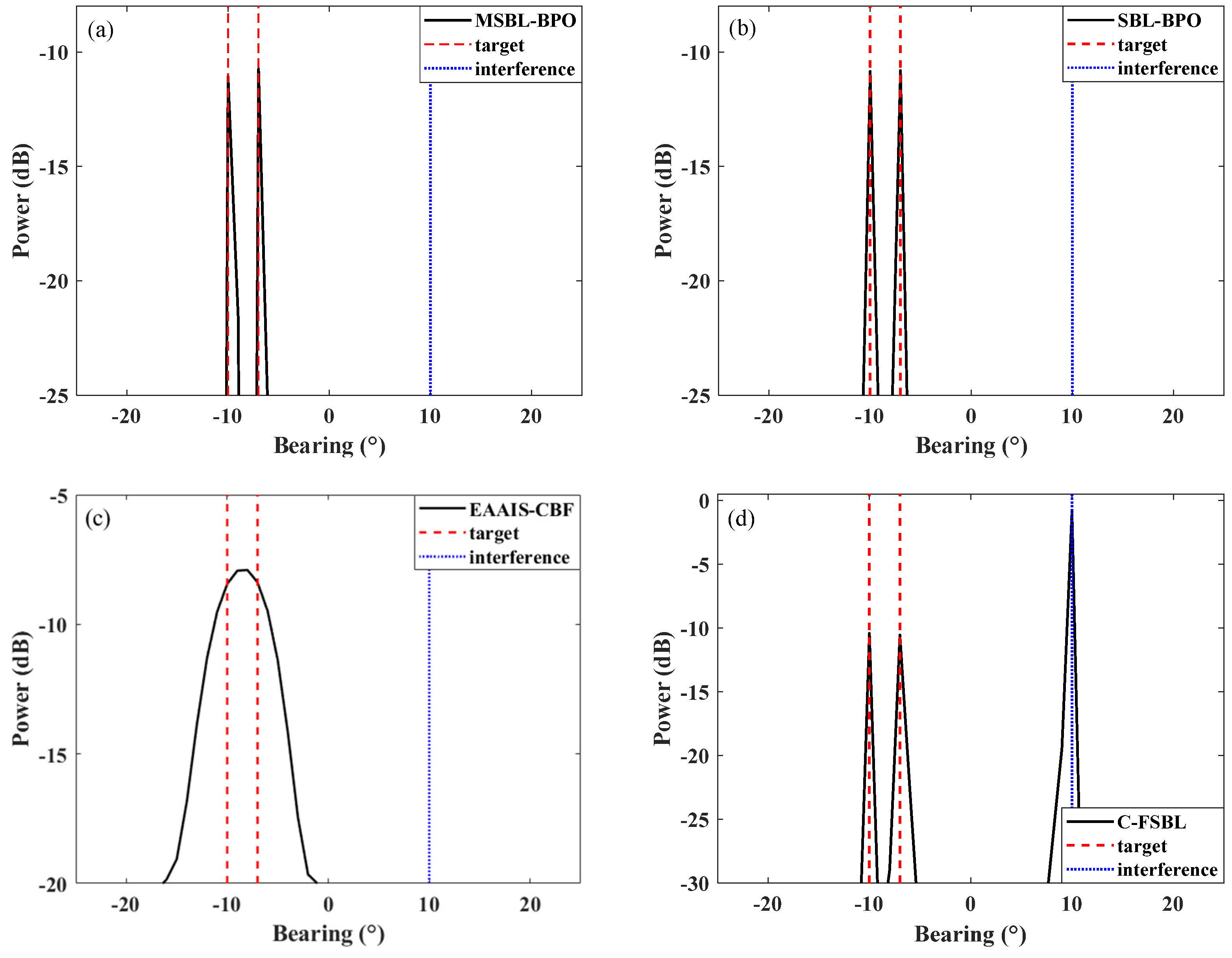
Figure 1 shows the spatial spectra of the abovementioned algorithms with SIR of −10 dB. The SNR and the number of snapshots N are set to −10 dB and 50, respectively. Under such a condition, the MSBL-BPO, the SBL-BPO and the C-FSBL as super-resolution methods, can estimate the two directions of the targets. On the contrary, though the EAAIS-CBF can suppress the interference by removing the interference subspace from the covariance matrix, it still cannot resolve the directions of signals because of the wide main lobe, which results in low resolution.

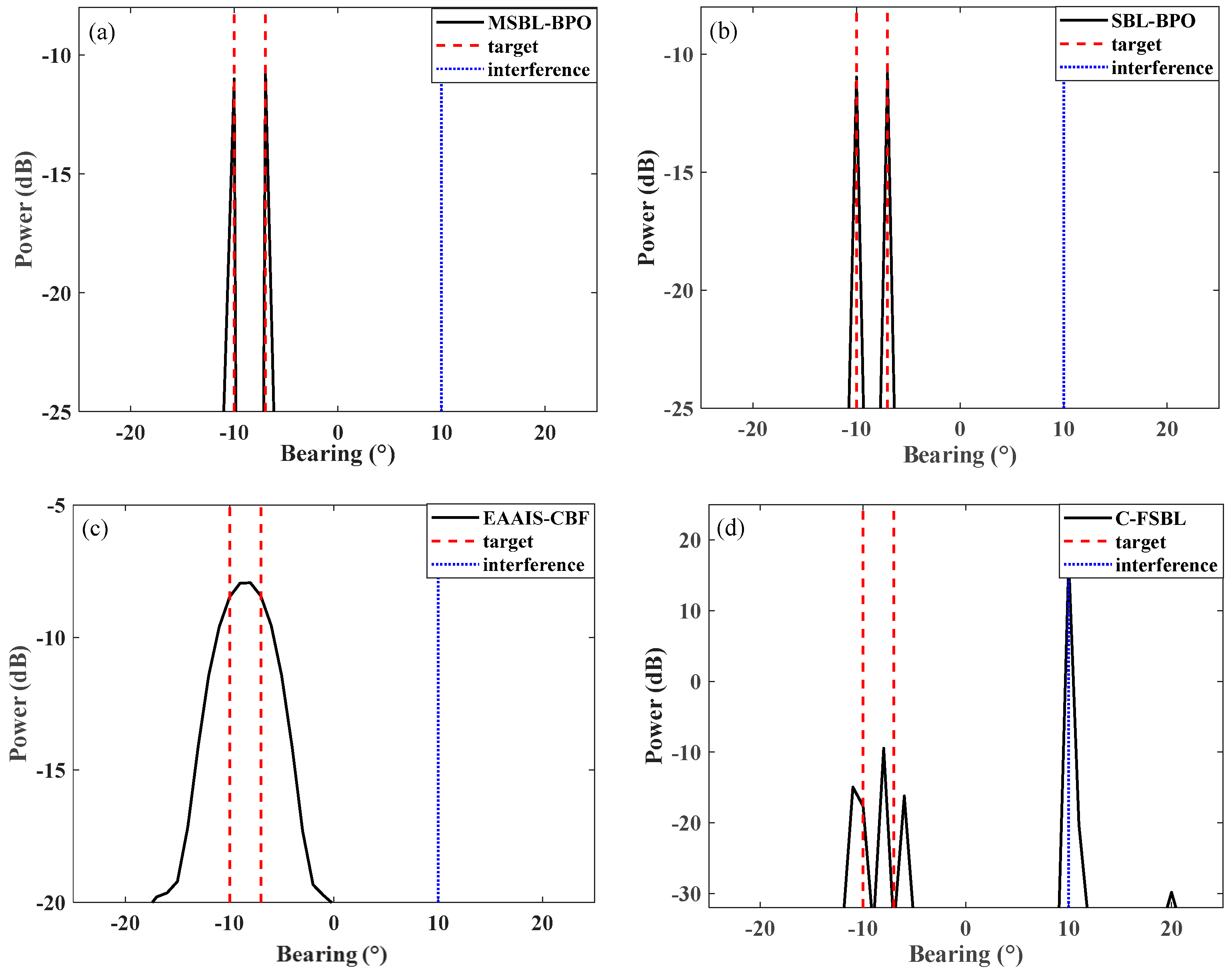
Then, the SIR increases to −30 dB. Figure 2 shows the spatial spectra of the method considered above under such a condition. Obviously, the interference power increases with a decrease in SIR. Once again, the proposed method and the SBL-BPO use the MVDR-DL as preprocessor to suppress the interference. As such, they can maintain good performance when the interference power increases. The C-FSBL can estimate the direction of the interference. However, its performance is seriously affected by the strong interference in comparison with the result in Figure 1d. The method experiences problems in resolving two directions of the targets. Furthermore, the EAAIS-CBF still cannot work under such a condition, mainly due to the low resolution.

Subsequently, the estimation accuracy of the methods is compared under different SIR conditions, examined by the root-mean-square error (RMSE):

$$\mathrm{RMSE}=\sqrt{\frac{1}{KW}{\displaystyle {\sum }_{k=1}^K{\displaystyle {\sum }_{w=1}^W{({\hat{\theta }}_k^w-{\theta }_k)}^2}}},$$

(42)

where K and W are the number of signals and the sum of the Monte Carlo runs, respectively. K = 2 and W = 200 in the simulations.

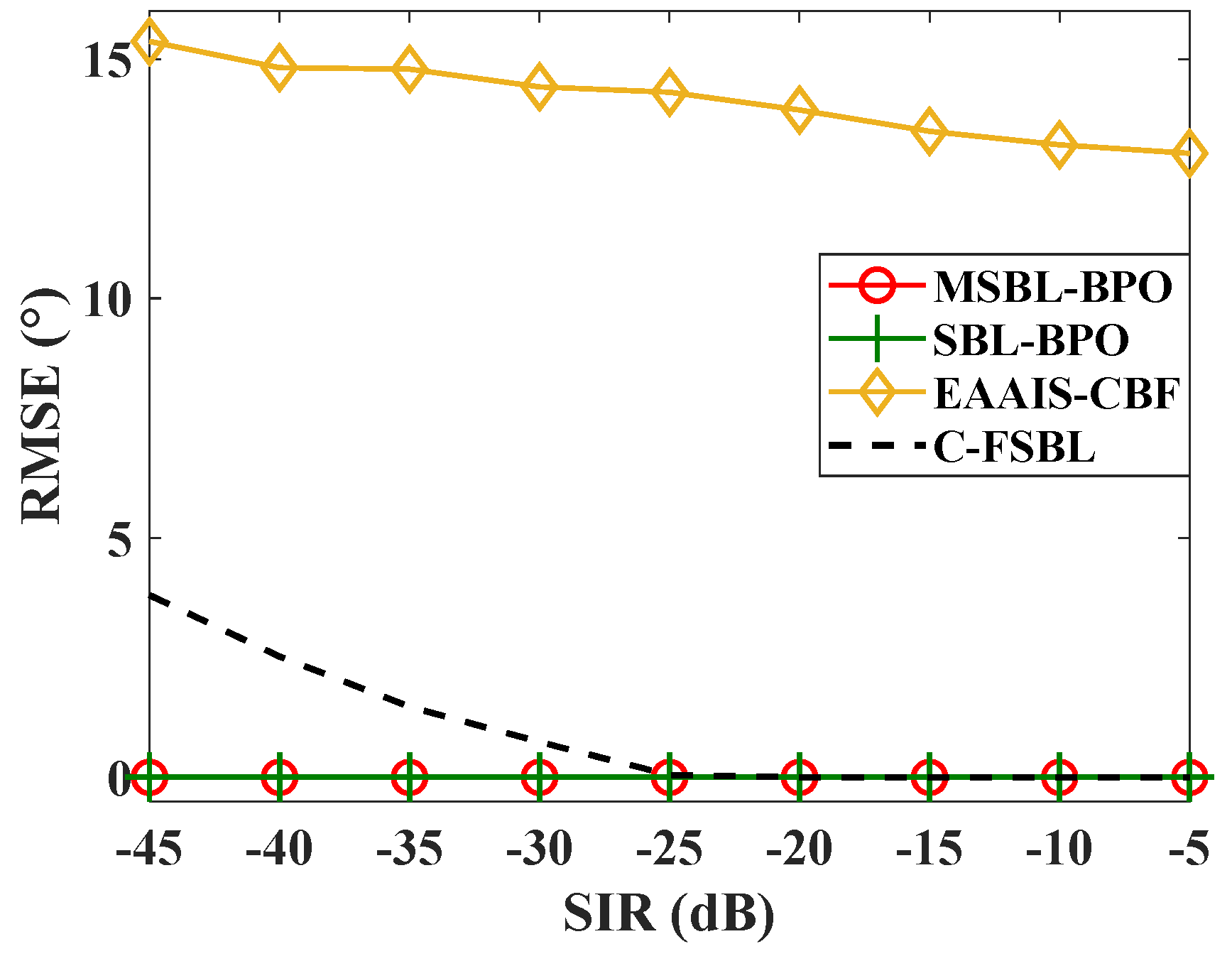
Figure 3 shows the RMSE of each method versus the SIR curve obtained by fixing the SNR and the number of snapshots N to −10 dB and 50, respectively. It can be observed that the performance of the MSBL-BPO is comparable to that of the SBL-BPO. They provide stable DOA estimates as the interference power increases since the interference is sufficiently suppressed by the MVDR-DL and cannot affect the DOA estimation. However, the performance of the C-FSBL is affected by strong interference, and its estimation precision decreases when SIR is smaller than −25 dB. The RMSEs of EAAIS-CBF are larger than in other methods. This is mainly because that the main lobe of the CBF is wide and only a peak exists in the sector [−14, −2]°, as shown in Figure 1c and Figure 2c. The peak out of the sector is mistaken for the target, leading to a large bias.

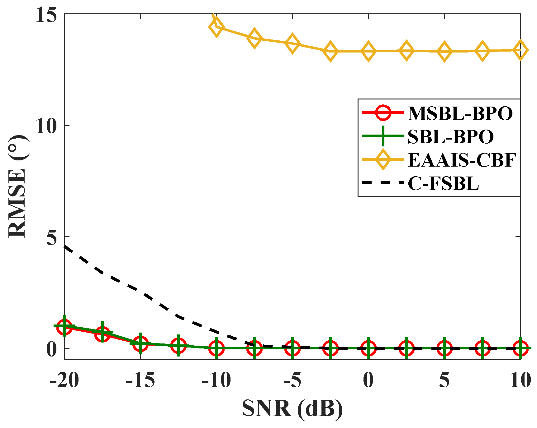
Figure 4 illustrates the RMSE of each method versus the SNR by fixing the SIR to −30 dB. Other parameters remain unchanged. The MSBL-BPO and the SBL-BPO use the MVDR-DL to suppress the interference, thus improving the signal-to-interference-and-noise ratio. Hence, they can be applied under lower SNR condition in comparison with other methods. Their RMSEs are lower than those of other methods when $\mathrm{SNR}<-2.5 \mathrm{dB}$. The performance of the C-FSBL is worse than that of the proposed method, since it directly estimates the DOAs from the received data and ignores the interference. The existence of the interference affects its performance, especially in low SNR cases. Furthermore, the EAAIS-CBF has a wide main lobe, which leads to low resolution. Hence, it cannot provide DOA estimates for the targets.

Finally, the computational efficiency is compared in terms of the running time. The simulation settings are the same as those shown in Figure 1. The mean running time over 200 trials is shown in

Table 1. Mean running time of each algorithm over 200 trials.

MSBL-BPO	SBL-BPO	EAAIS-CBF	C-FSBL
0.17 s	0.48 s	0.13 s	0.78 s

. The time usage of the proposed method is almost three times smaller than that of the SBL-BPO. This is mainly because the SBL-BPO applies the VBI to estimate the parameters in Equation (12) and the workload almost depends on Equation (14), i.e., $O\left(L{K}_G^3\right)$ in each iteration. In contrast, as shown in Algorithm 1, the proposed method avoids matrix inversion. At this time, the computational workload of ${\Sigma }_l^{(i)}$ updating is $O\left(L{K}_{active}{K}_B\right)$ if a basis is added to the active basis set in an iteration, while the computational workload becomes $O\left(L{K}_{active}^2\right)$ if a basis is updated or deleted, where $K_{active}$ represents the number of elements in active basis set. It is obvious that the workload of the proposed method is smaller than that of the SBL-BPO since $K_{active},K_B<K_G$. Hence, the proposed method successfully improves the computational efficiency in comparison with SBL-BPO. Though C-FSBL also avoids matrix inversion, this method uses the vectorized covariance matrix model, increasing the dimension of the matrix. The workload of this method is $O\left(L{K}_{active}{M}^2\right)$ if a basis is added to the active basis set in an iteration, while the computational workload is $O\left(L{K}_{active}^2\right)$ when a basis is updated or deleted. Hence, its computational workload is also larger than that of the proposed method, since $K_B<M$. Furthermore, the EAAIS-CBF achieves high computational efficiency because it needs no iteration to estimate DOAs and the workload mainly depends on eigen decomposition. Therefore, the proposed method can achieve high estimation precision in the strong interference environment. At the same time, it achieves high computational efficiency, which is comparable to the traditional method.

5. Experimental Results

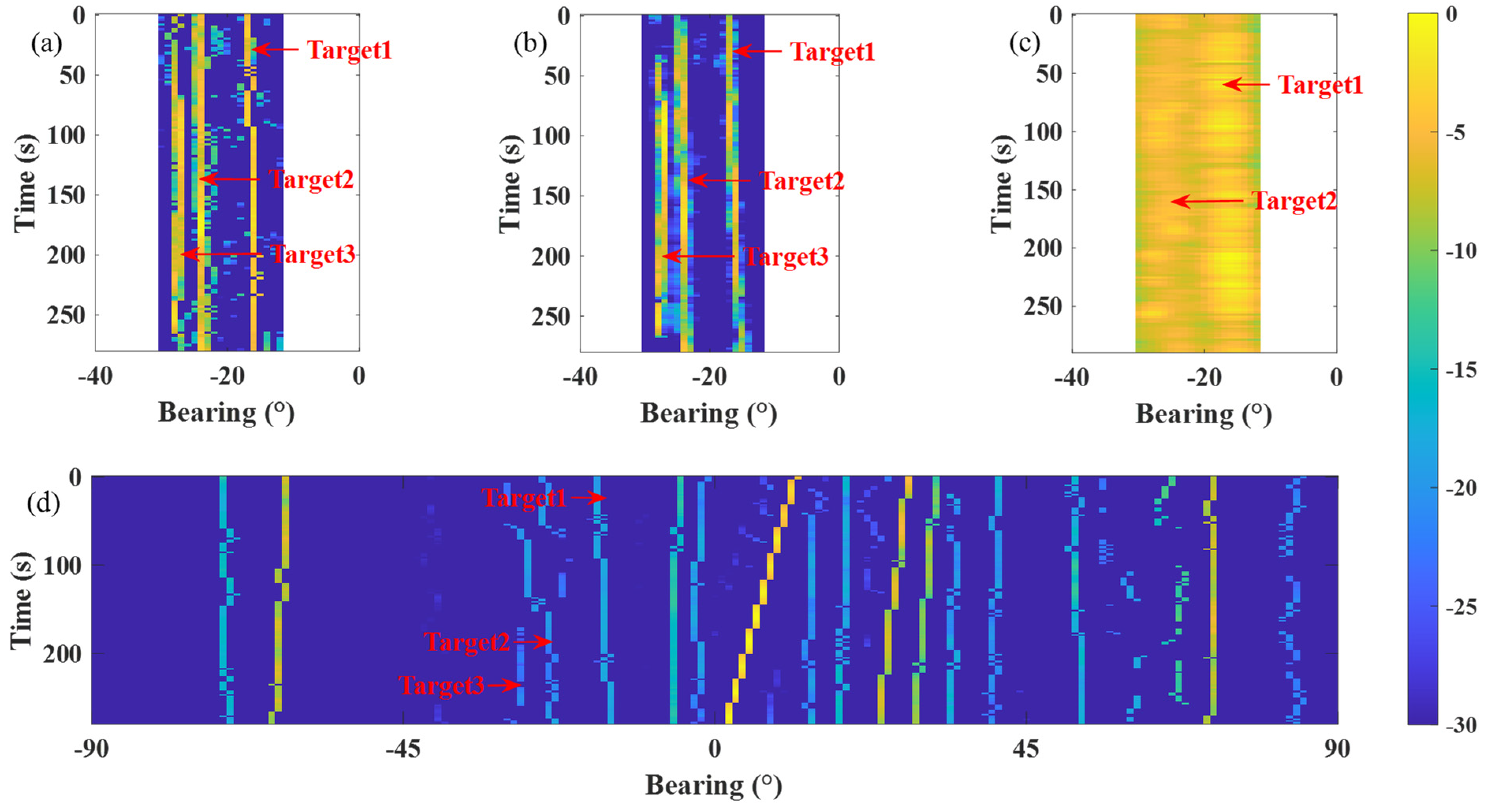
Experimental data were collected by a tow array with 32 hydrophones uniformly spaced at 4 m, which was processed in [32]. Target1, target2 and target3 were, respectively, located at −18°, −25°, and −29°. The received data sampled at 2048 Hz, are divided into 96 frames with 15 s of data, and the overlap between the adjacent frames is 80%. The data in each frame are divided into 49 blocks with 50% overlap, i.e., N = 49. A 1024-point DFT is applied in each block, i.e., the frequency resolution is 2 Hz. The analyzed frequency ranges from 90 to 180 Hz. The sector-of-interest in MSBL-BPO and SBL-BPO is set to [−30, −12]°. The sector is divided with a step of 2° to obtain beam pointing angles. The coarse bearing range in EAAIS-CBF is also set to [−30, −12]°. Other parameter settings remain the same as those in the simulations.

Figure 5 illustrates the DOA estimation result of each method. The MSBL-BPO and SBL-BPO use the MVDR-DL as preprocessor to sufficiently suppress the interferences, thus decreasing the influence of the interference on DOA estimation. They can estimate three weak targets well. In contrast, the performance of C-FSBL is affected by the interference, and it has some difficulties in resolving target2 and target3 from 120 s to 150 s. The EAAIS-CBF removes the interference subspace from the covariance matrix, thus preventing the interference from masking the targets to some degree. Unfortunately, the main lobe of its spatial spectrum is wide. Hence, it cannot resolve target2 and target3 due to the low resolution.

Table 2. Mean running time of each algorithm over frames.

MSBL-BPO	SBL-BPO	EAAIS-CBF	C-FSBL
0.19 s	0.63 s	0.17 s	0.92 s

shows the mean running time of each algorithm over segments. Similar to the simulation result, the computational efficiency of the proposed method is comparable to that of EAAIS-CBF, but the EAAIS-CBF suffers from low resolution, as shown before. The time usage of the MSBL-BPO is almost three times smaller than that of the SBL-BPO, since the proposed method avoids matrix inversion. The mean running time of the C-FSBL is longer than that of the proposed method due to the large matrix dimension. Hence, we can draw a conclusion that the proposed method can achieve better performance than state-of-the-art methods in a strong interference environment.

6. Conclusions

DOA estimation in a strong interference environment is a difficult problem to be solved. Under such conditions, strong interference will mask the target-of-interest and the DOAs of the targets can hardly be obtained, leading to a significant challenge to weak target detection for the passive sonar system. The SBL-BPO is a useful tool to estimate DOAs in a strong interference environment. This method uses the MVDR-DL beamformer to suppress interference and estimates the DOAs from BPO in the Bayesian framework. However, it needs to compute matrix inversion in each iteration, which brings some computational burden to the system. This paper modifies the SBL-BPO to reduce this computational burden. The Fast-RVM is extended to the beam domain, and then a sequential solution for the BPO probabilistic model is provided in this paper. As such, only single signal precision parameter is updated in each iteration and matrix inversion computation is avoided. Simulation and experimental results verify that the MSBL-BPO can provide stable DOA estimates for targets in a strong interference environment, thus improving the ability of the sonar system in weak target detection. Meanwhile, its computational efficiency is comparable to the subspace-separation-based method. Hence, the proposed method successfully reduces computational burden for the system and has potential in practical signal processing. In future work, the DOA estimation problem should be further researched under the condition where the target and interference are coherent in order to increase the anti-interference ability of the system.

References

1. Gerstoft, P.; Xenaki, A.; Mecklenbräuker, C.F. Multiple and single snapshot compressive beamforming. J. Acoust. Soc. Am. 2015, 138, 2003–2014. [Google Scholar] [CrossRef] [PubMed]
2. Yang, Y.; Zhang, Y.; Yang, L.; Wang, Y. Wideband direction-of-arrival estimation based on hierarchical sparse Bayesian learning for signals with the same or different frequency bands. Electronics 2023, 12, 1123. [Google Scholar] [CrossRef]
3. Wang, Q.; Yu, H.; Li, J.; Ji, F.; Chen, F. Adaptive Grid Refinement Method for DOA Estimation via Sparse Bayesian Learning. IEEE J. Oceanic Eng. 2023, 48, 806–819. [Google Scholar] [CrossRef]
4. Guo, M.; Sun, Y.; Dai, J.; Chang, C. Robust DOA estimation for burst impulsive noise. Digit. Signal Process. 2021, 114, 103059. [Google Scholar] [CrossRef]
5. Dai, J.; So, H.C. Real-valued sparse Bayesian learning for DOA estimation with arbitrary linear arrays. IEEE Trans. Signal Process. 2021, 69, 4977–4990. [Google Scholar] [CrossRef]
6. Fortuna, L.; Buscarino, A. Automatic Control and System Theory and Advanced Applications—Volume 2. Electronics 2024, 9, 5. [Google Scholar] [CrossRef]
7. Zheng, J.; Kaveh, M. Sparse spatial spectral estimation: A covariance fitting algorithm, performance and regularization. IEEE Trans. Signal Process. 2013, 61, 2767–2777. [Google Scholar] [CrossRef]
8. Malioutov, D.; Cetin, M.; Willsky, A.S. A sparse signal reconstruction perspective for source localization with sensor arrays. IEEE Trans. Signal Process. 2005, 53, 3010–3022. [Google Scholar] [CrossRef]
9. He, Z.; Shi, Z.; Huang, L.; So, H.C. Underdetermined DOA estimation for wideband signals using robust sparse covariance fitting. IEEE Signal Process. Lett. 2015, 22, 435–439. [Google Scholar] [CrossRef]
10. Ling, Y.; Gao, H.; Ru, G.; Chen, H.; Li, B.; Cao, T. Grid reconfiguration method for off-grid DOA estimation. Electronics 2019, 8, 1209. [Google Scholar] [CrossRef]
11. Chen, P.; Chen, Z.; Zhang, X.; Liu, L. SBL-based direction finding method with imperfect array. Electronics 2018, 7, 426. [Google Scholar] [CrossRef]
12. Wang, Q.; Yu, H.; Li, J.; Ji, F.; Chen, F. Sparse Bayesian learning using generalized double Pareto prior for DOA estimation. IEEE Signal Process. Lett. 2021, 28, 1744–1748. [Google Scholar] [CrossRef]
13. Bai, Z.; Shi, L.; Jensen, J.R.; Sun, J.; Christensen, M.G. Acoustic DOA estimation using space alternating sparse Bayesian learning. EURASIP J. Audio Speech Music. Process. 2021, 2021, 14. [Google Scholar] [CrossRef]
14. Das, A.; Sejnowski, T.J. Narrowband and wideband off-grid direction-of-arrival estimation via sparse Bayesian learning. IEEE J. Oceanic Eng. 2018, 43, 108–118. [Google Scholar] [CrossRef]
15. Das, A. Real-valued sparse Bayesian learning for off-grid direction-of-arrival (DOA) estimation in ocean acoustics. IEEE J. Oceanic Eng. 2021, 46, 172–182. [Google Scholar] [CrossRef]
16. Hu, N.; Sun, B.; Zhang, Y.; Dai, J.; Wang, J.; Chang, C. Underdetermined DOA estimation method for wideband signals using joint nonnegative sparse Bayesian leaning. IEEE Signal Process. Lett. 2017, 24, 535–539. [Google Scholar] [CrossRef]
17. Choo, Y.; Yang, H. Broadband off-grid DOA estimation using block sparse Bayesian learning for nonuniform noise variance. IEEE J. Oceanic Eng. 2022, 47, 1024–1040. [Google Scholar] [CrossRef]
18. Wipf, D.; Rao, B.D. Sparse Bayesian learning for basis selection. IEEE Trans. Signal Process. 2004, 52, 2153–2164. [Google Scholar] [CrossRef]
19. Tzikas, D.G.; Likas, A.C.; Galatsanos, N.P. The variational approximation for Bayesian inference. IEEE Signal Process. Mag. 2008, 25, 131–146. [Google Scholar] [CrossRef]
20. Figueiredo, M.A. Adaptive sparseness for supervised learning. IEEE Trans. Pattern Anal. Mach. Intell. 2003, 25, 1150–1159. [Google Scholar] [CrossRef]
21. Jiang, Y.; He, M.; Liu, W.; Han, J.; Feng, M. Underdetermined wideband DOA estimation for off-grid targets: A computationally efficient sparse Bayesian learning approach. IET Radar Sonar Navig. 2020, 14, 1583–1591. [Google Scholar] [CrossRef]
22. Tipping, M.E.; Faul, A.C. Fast marginal likelihood maximisation for sparse Bayesian models. In Proceedings of the 9th International Workshop on Artificial Intelligence and Statistics, Key West, FL, USA, 3–6 January 2003. [Google Scholar]
23. Harrison, B.F. The eigencomponent association method for adaptive interference suppression. J. Acoust. Soc. Am. 2004, 115, 2122–2128. [Google Scholar] [CrossRef]
24. Ren, S.; Ge, F.; Guo, X.; Guo, L. Eigenanalysis-based adaptive interference suppression and its application in acoustic source range estimation. IEEE J. Oceanic Eng. 2015, 40, 903–916. [Google Scholar] [CrossRef]
25. Kim, H.; Viberg, M. Two decades of array signal parameter estimation. IEEE Signal Process. Mag. 1996, 13, 67–94. [Google Scholar]
26. Yang, L.; Yang, Y.; Zhu, J. Source localization based on sparse spectral fitting and spatial filtering. In Proceedings of the Oceans 2016 MTS/IEEE Monterey, Monterey, CA, USA, 19–23 September 2016; pp. 1–4. [Google Scholar]
27. Yang, Y.; Zhang, Y.; Yang, L. Wideband sparse spatial spectrum estimation using matrix filter with nulling in a strong interference environment. J. Acoust. Soc. Am. 2018, 143, 3891–3898. [Google Scholar] [CrossRef] [PubMed]
28. Macinnes, C.S. Source localization using subspace estimation and spatial filtering. IEEE J. Oceanic Eng. 2004, 29, 488–497. [Google Scholar] [CrossRef]
29. Hassanien, A.; Elkader, S.A.; Gershman, A.B. Convex optimization based beam-space preprocessing with improved robustness against out-of-sector source. IEEE Trans. Signal Process. 2006, 54, 1587–1595. [Google Scholar] [CrossRef]
30. Yuan, J.; Xiao, H.; Cai, Z.; Xi, C. DOA estimation based on multiple beamspace measurements sparse reconstruction for manoeuvring towed array. J. Phys. Conf. Ser. 2017, 787, 012026. [Google Scholar] [CrossRef]
31. Compaleo, J.; Gupta, I.J. Application of sparse representation to Bartlett spectra for improved direction of arrival estimation. Sensors 2021, 21, 77. [Google Scholar] [CrossRef] [PubMed]
32. Zhang, Y.; Yang, Y.; Yang, L.; Wang, Y. Sparse Bayesian learning for wideband direction-of-arrival estimation via beamformer power outputs in a strong interference environment. Jasa Express Lett. 2022, 2, 014801. [Google Scholar] [CrossRef] [PubMed]
33. Carlson, B.D. Covariance matrix estimation errors and diagonal loading in adaptive arrays. IEEE Trans. Aerosp. Electron. Syst. 1988, 24, 397–401. [Google Scholar] [CrossRef]
Figure 1. The spatial spectra of (a) MSBL-BPO, (b) SBL-BPO, (c) EAAIS-CBF, and (d) C-FSBL with the SIR of −10 dB. Two dashed lines represent the directions of the targets, and the dotted line shows the direction of the interfering source.
Electronics 13 01456 g001
Figure 2. The spatial spectra of (a) MSBL-BPO, (b) SBL-BPO, (c) EAAIS-CBF, and (d) C-FSBL with the SIR of −30 dB. Two dashed lines represent the directions of the targets, and the dotted line shows the direction of the interfering source.
Electronics 13 01456 g002
Figure 3. RMSE of DOA estimates versus SIR.
Electronics 13 01456 g003
Figure 4. RMSE of DOA estimates versus SNR.
Electronics 13 01456 g004
Figure 5. Bearing and time recordings of (a) MSBL-BPO, (b) SBL-BPO, (c) EAAIS-CBF, and (d) C-FSBL. The red arrows indicate the estimated DOAs.
Electronics 13 01456 g005