MDP-SLAM: A Visual SLAM towards a Dynamic Indoor Scene Based on Adaptive Mask Dilation and Dynamic Probability

Abstract

Visual simultaneous localization and mapping (SLAM) algorithms in dynamic scenes will apply the moving feature points to the camera pose’s calculation, which will cause the continuous accumulation of errors. As a target-detection tool, mask R-CNN, which is often used in combination with the former, due to the limited training datasets, easily results in the semantic mask being incomplete and deformed, which will increase the error. In order to solve the above problems, we propose in this paper a visual SLAM algorithm based on an adaptive mask dilation strategy and the dynamic probability of the feature points, named MDP-SLAM. Firstly, we use the mask R-CNN target-detection algorithm to obtain the initial mask of the dynamic target. On this basis, an adaptive mask-dilation algorithm is used to obtain a mask that can completely cover the dynamic target and part of the surrounding scene. Then, we use the K-means clustering algorithm to segment the depth image information in the mask coverage area into absolute dynamic regions and relative dynamic regions. Combined with the epipolar constraint and the semantic constraint, the dynamic probability of the feature points is calculated, and then, the highly dynamic possible feature points are removed to solve an accurate final pose of the camera. Finally, the method is tested on the TUM RGB-D dataset. The results show that the MDP-SLAM algorithm proposed in this paper can effectively improve the accuracy of attitude estimation and has high accuracy and robustness in dynamic indoor scenes.

1. Introduction

Simultaneous localization and mapping (SLAM) systems are now widely used in many robotics technologies. Depending on the device used for data collection, current SLAM technologies are mainly divided into two types. The first type uses LiDAR to detect the distance; however, this type of SLAM is expensive and is often used for autonomous driving technology. The second type is a visual SLAM system that uses a camera as a sensor, which is less expensive than LiDAR SLAM and is small and portable. With continuous development, many mature SLAM algorithms have been developed, such as LSD-SLAM [1], ORB-SLAM2 [2], and MonoSLAM [3].

Most visual SLAM systems are assumed to be used in completely static work scenes, so the changes in the surrounding environment cause them to continuously accumulate errors, which inevitably reduces the accuracy and reliability of the system. With respect to this problem, visual SLAM has been considered and studied continuously in the past few years. With the development of machine learning in recent years, more and more visual SLAM methods integrating deep learning have been proposed to solve this problem, and SLAM methods using semantic constraints are a typical representative. Semantic information is mainly used to identify and remove potential dynamic objects in the scene. The semantic prior information obtained by object detection and semantic segmentation can provide more accurate object masks. Especially in depth images, the contours of a dynamic object are usually easily distinguished from the surrounding environment, which provides a favorable guide for further improvement of the object contours obtained by semantic segmentation. However, due to the limited types of known objects and training datasets, the mask obtained may have some problems, such as failing to cover the dynamic objects completely and reducing the available static feature points due to excessive blocking of the image.

In order to solve the above problems and improve the pose estimation accuracy and robustness of visual SLAM systems for indoor dynamic scenes, the main contributions of the proposed method are as follows:

(1) We combine the depth information of the image with the initial mask of the dynamic object and its position information in the frame provided by the mask R-CNN [4] object-detection algorithm and accurately segment the contour of the dynamic object from the static background by using the K-means clustering algorithm.

(2) An adaptive mask-dilation algorithm is proposed, which takes the changes of the mask of the dynamic object in the previous three key frames as the reference and outputs the suggested dilation coefficient of the mask in the current frame. By using this algorithm, a mask that can cover the dynamic object completely can be obtained, while avoiding that the depth information in the mask region is too complicated.

(3) A dynamic feature point-filtering strategy based on an epipolar constraint and a semantic constraint is proposed. Then, the remaining feature points are used to solve the final pose of the camera.

The rest of this paper is organized as follows. Section 2 describes the related work. Section 3 describes the details of MDP-SLAM. Section 4 gives the experimental results and analysis. Finally, the experimental conclusions are given in Section 5.

2. Related Works

Dynamic SLAM algorithms can be broadly divided into two types: traditional methods, which do not use deep learning models, and fusion methods, which use deep learning models. The latter relies on the semantic prior information provided by the deep learning models, such as detection boxes with semantic labels or the generated object masks for dynamic segmentation.

2.1. Dynamic SLAM Based on Conventional Method

When the prior information of dynamic targets cannot be obtained, improving the accuracy of visual SLAM mainly depends on finding reliable static feature points for matching. DMS-SLAM [5] uses sliding windows between two non-adjacent frames to detect matching feature points and, then, uses GMS [6] to remove the outliers. Sun et al. [7] proposed a dynamic filtering method based on RGB-D data to remove dynamic pixels by establishing a foreground model. Wang et al. [8] proposed two fundamental matrix constraints to filter the dynamic objects and, then, used the distribution of the points with mismatches to locate the dynamic region, and the dynamic region contour was finally segmented by the depth-information-clustering method. This work makes use of the mismatching points that are usually ignored and cleverly obtains the dynamic regions that are prone to being mismatched.

In addition, the optical flow method is also one of the commonly used methods. Cheng et al. [9] used the optical flow vector and the essential matrix to detect the dynamic feature points. Wang et al. [10] used the optical-flow-motion-description vector to randomly sample the feature points and select the category with the most inner points as a static reference. Although the use of the optical flow can result in good dynamic segmentation, when the light in the scene suddenly changes or the camera shakes violently, these methods can easily lose accuracy.

2.2. Dynamic SLAM Based on Deep Learning Model

In recent years, with the wide application of deep learning in the field of computer vision, the accuracy and efficiency of dynamic target detection have been continuously improved. Many methods have been proposed to use semantic constraints and object detection for preprocessing to eliminate potential dynamic objects in the scene, methods such as PWC-NET [11], Deeplabv3 [12], and mask R-CNN have been gradually integrated into visual SLAM. Bescos et al. [13] overlaid the semantic mask generated by mask R-CNN on dynamic objects under the constraint of multi-view geometry to avoid using dynamic feature points. Other methods that combine mask R-CNN with geometric constraints include MaskFusion [14] and DP-SLAM. In addition, YOLACT [15], YOLO [16], and SSD [17] are all deep learning models that are widely used in conjunction with visual SLAM. These works focus on the integration of semantic information obtained through deep learning methods into the system for use, and there is no in-depth exploration of the further improvement of the constraints.

In this environment, how to use semantic information efficiently becomes particularly important. The dynamic probability propagation method proposed by Li et al. [18] can assign appropriate weights to the geometric and semantic constraint results according to the environmental conditions in the whole process to obtain the final dynamic probability, and this makes up for the shortcomings of the two constraint methods. Yang et al. [19] established a motion possibility model using semantic information, assigned different initial static weight values to different types of objects, and adjusted the motion possibility and dynamic weight according to the motion of objects in the whole process to reduce the interference of dynamic feature points. Both of the above methods establish further probabilistic constraints on dynamic objects while utilizing semantic information. DM-SLAM [20] and SDF-SLAM [21] further improve the effect of common geometric constraint methods on the basis of the fusion of semantic segmentation, and these works show that the combination of deep learning models and traditional methods allow visual SLAM to have broader application scenarios.

3. Methodology

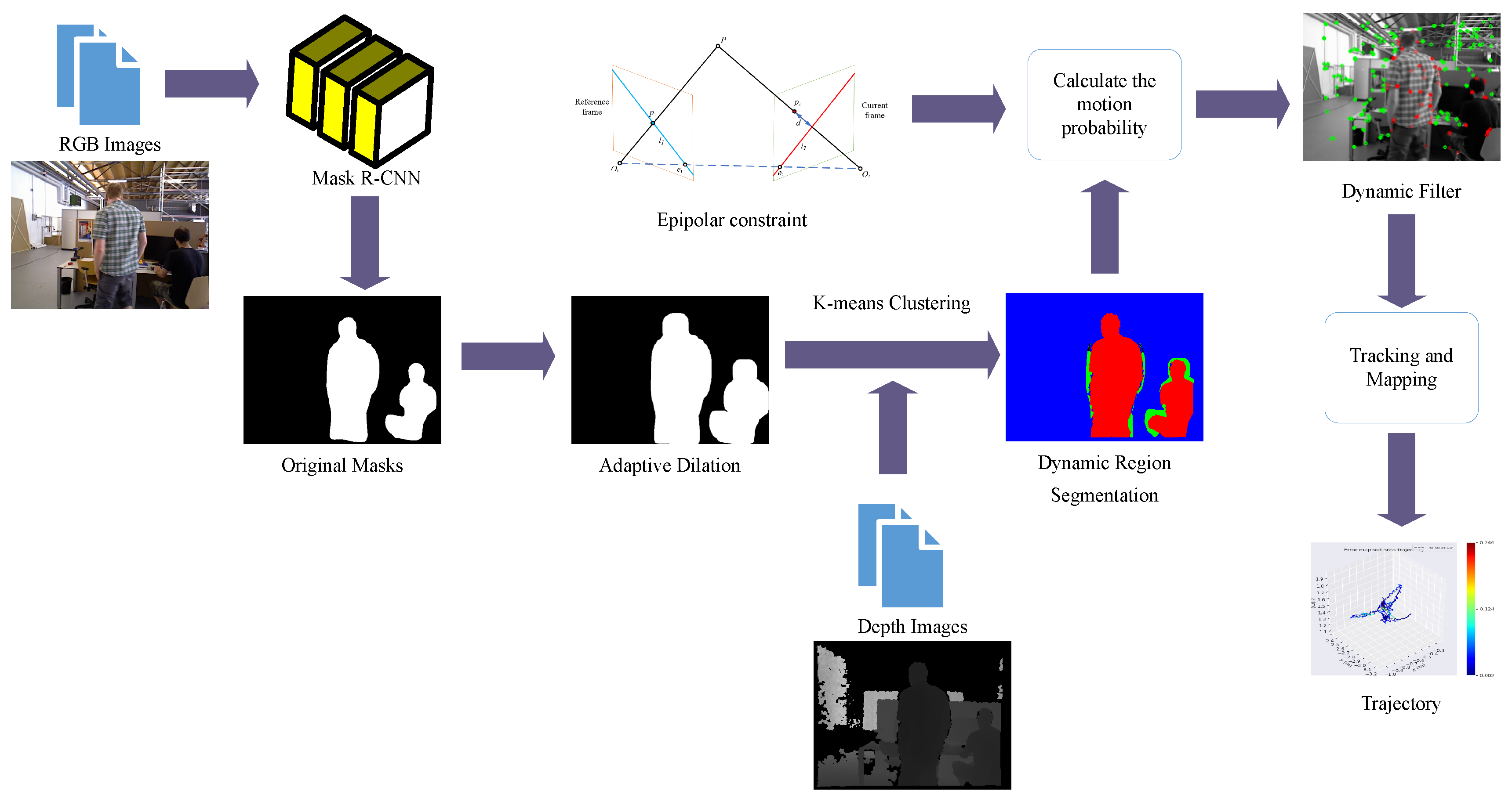
3.1. Overview of Framework

The framework of MDP-SLAM is shown in Figure 1. The RGB images are input into the mask R-CNN network for semantic segmentation to obtain the initial mask firstly. The initial mask is then processed by the adaptive dilation algorithm and combined with the input depth image to obtain the result of dynamic region segmentation through the K-means clustering algorithm. Meanwhile, the red dynamic feature points are filtered out according to the geometric constraint. The green static feature points are retained for subsequent pose calculation.

Based on ORB-SLAM2, the mask R-CNN object-detection algorithm and the K-means clustering algorithm incorporating adaptive mask dilation are added into the preprocessing module. In the pose-solving module, a dynamic probability calculation algorithm based on semantic and geometric constraints is added. The workflow of MDP-SLAM is described as follows: First, the initial mask of the dynamic object is generated by the mask R-CNN network, processed by the adaptive mask dilation algorithm, and then, K-means clustering is used [22] with the depth image to segment the dynamic object from the static background. Then, the results of K-means clustering and the geometric constraint will work together to remove the dynamic feature points after the dynamic probability calculation. Finally, the retained feature points will be used to calculate the final pose.

The masks of the dynamic objects are obtained by using mask R-CNN, one of the most advanced object-detection networks available today, which can discern 80 different categories trained on the COCO dataset [23]. Ten categories were selected as potential dynamic objects, and for most indoor environments, the dynamic objects that may appear are included in these ten categories.

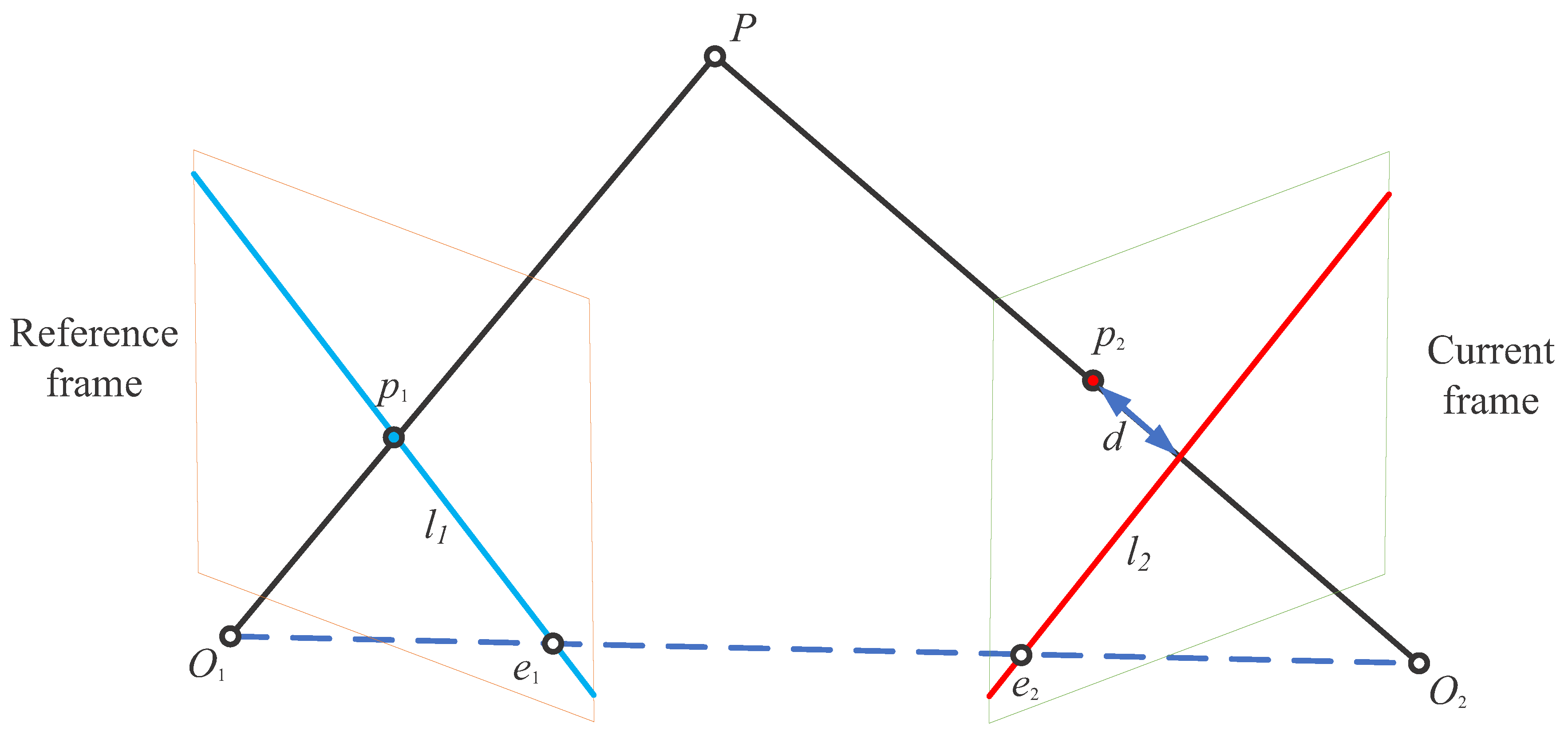
3.2. Geometric Constraint

Figure 2 shows the epipolar constraint between the reference frame and the current frame. $O_1$, $O_2$ are the optical center of the camera of the reference frame and the current frame, respectively; $p_1$ and $p_2$ are a pair of matching keypoints between the two frames; P is the mapping point of $p_1$ on the reference frame in three-dimensional space. A polar plane can be defined by $O_1$, $O_2$, and point P, and the line of $O_1$$O_2$ is called the baseline.

The matching points $p_1$ and $p_2$ are converted into homogeneous coordinates as follows:

$$P_1=\left[u_1,v_1,1\right], P_2=\left[u_2,v_2,1\right]$$

(1)

where u and v represent the pixel coordinates of the matching keypoints, and the epipolar line $L_i$ is determined by the following equation:

$$l_i=\left[\begin{array}{c}X\hfill \\ Y\hfill \\ Z\hfill \end{array}\right]=F{P}_i^T=F\left[\begin{array}{c}{u}_i\\ v_i\\ 1\end{array}\right](i=1,2)$$

(2)

where X, Y, Z represent a line vector and F represents a fundamental matrix. Then, the distance from the matching keypoints to the epipolar line is determined as follows:

$$D=\frac{\left|P_2^{T}F{P}_1\right|}{\sqrt{{\parallel X\parallel }^2+{\parallel Y\parallel }^2}}$$

(3)

Since the object may be in motion, the keypoints in the frame cannot accurately fall on the epipolar line, so the longer the offset distance is, the greater the moving probability is. It is assumed that the distance between the matching keypoints and the corresponding epipolar line satisfies the Gaussian distribution, and the dynamic probability of the keypoints is calculated by using the probability density function of the normal distribution, which is defined as follows:

$$P=\frac{1}{\sqrt{2\pi \delta }}exp\left(-\frac{D^2}{2{\delta }^2}\right)$$

(4)

where the parameter $\delta$ represents the standard deviation of this distribution, which is set to 1 in our experiment, and the mathematical expectation of this distribution is set to 0.

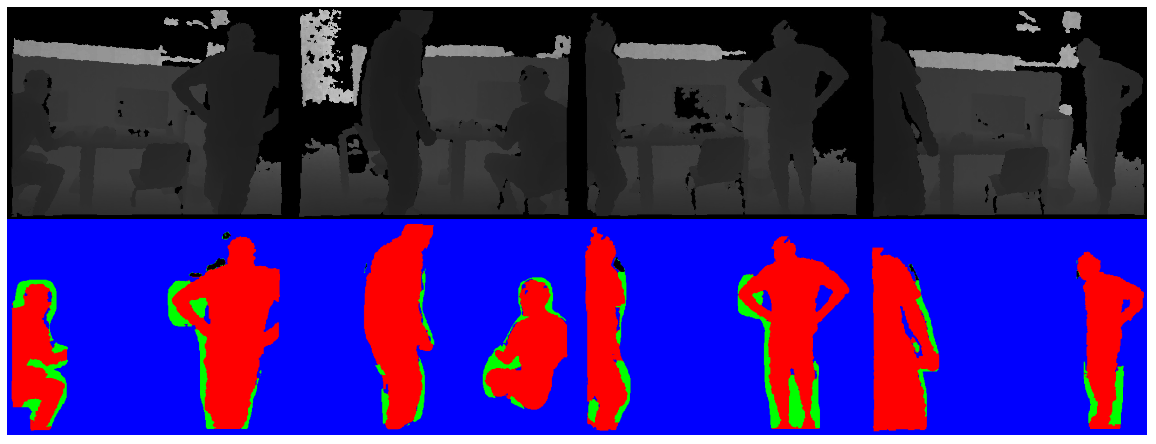
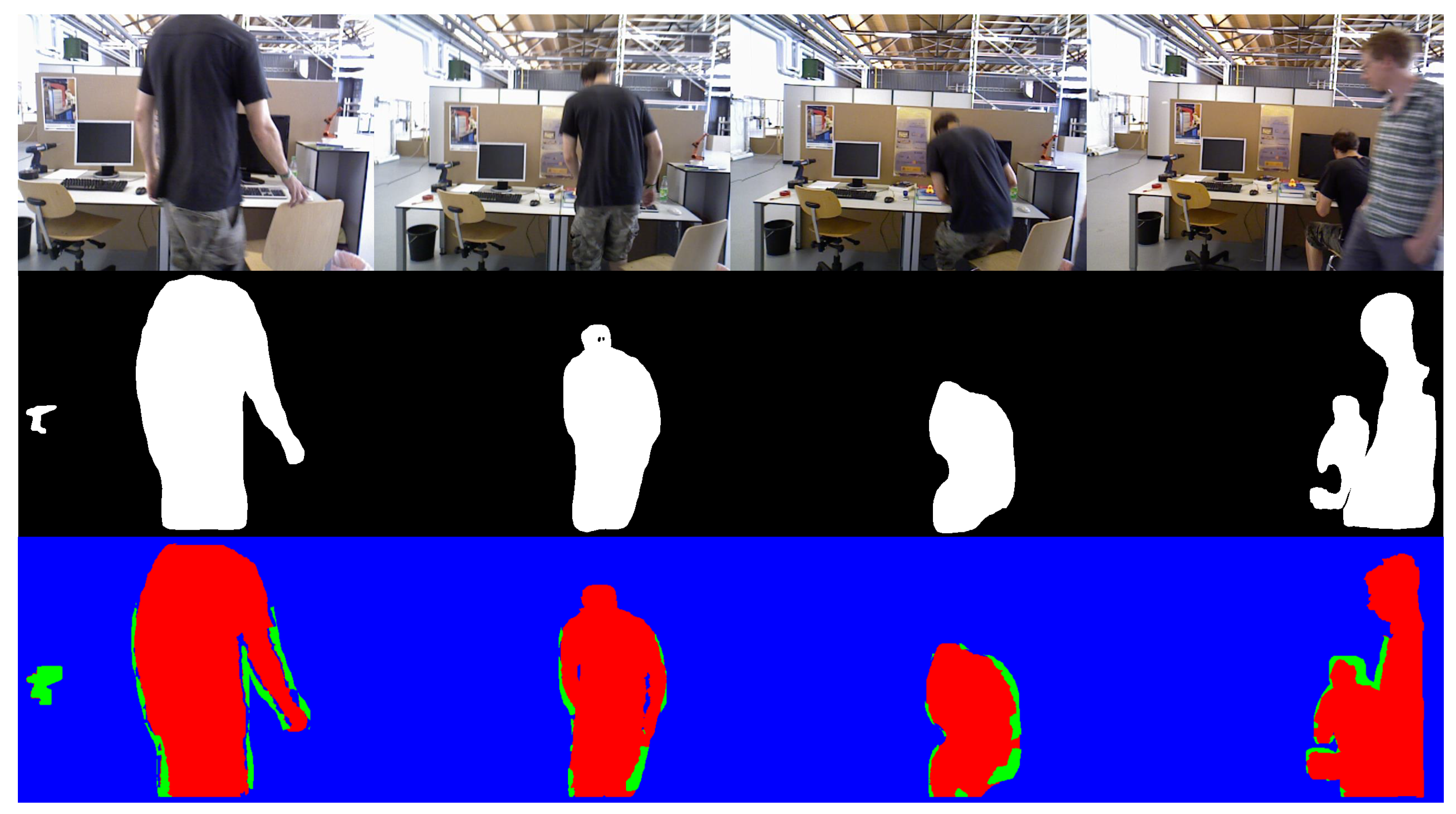
3.3. Segmentation of Dynamic Objects

The K-means clustering algorithm is a commonly used unsupervised learning algorithm used to divide samples in a dataset into K distinct groups (or clusters) such that each sample belongs to the cluster represented by its nearest mean (cluster center).

There is an obvious problem in using depth information to cluster depth images directly: due to the rich level of the scene depth in each scene, the number and distribution of objects at different levels are irregular, resulting in the failure of the clustering algorithm to accurately obtain the number of clusters. In practice, if the number of clusters is too small, a large number of objects with similar depth information will be linked together; if the number of clusters is too large, it will not be able to effectively unify the same kind of objects and use more computing resources.

The above problems directly lead to the inability to obtain accurate dynamic object masks based on clustering algorithms, and the emergence of deep learning networks makes up for this problem. The adaptive dilation algorithm proposed in this paper processes the initial dynamic mask generated by the mask R-CNN semantic segmentation module, avoids the mutual interference of depth information, and contains only a few targets, which provides a good environment for the use of the K-means clustering algorithm based on depth information.

In order to further improve the accuracy of the results obtained by the K-means clustering algorithm, we improved the method of obtaining the number of clusters K. The steps are as follows:

(1) Obtain the total number of all pixels N and the maximum depth value $d_{max}$ in the mask-covered region after using the adaptive dilation algorithm in the current frame.

(2) The first thing to determine is the number of clusters in the first frame. Since the mask region does not contain depth information complex enough to interfere with the number of clusters, we process the initial cluster number in accordance as 3, 4, and 5, respectively, and pay attention to the coincidence of the cluster and dynamic object initial mask under different settings. This choice is due to a depth image of a scene usually being composed mainly of the near-part closest to the lens, the far-part farthest from the lens, and the middle part, and scenes in the middle may also have significantly different depths. If a cluster generated under a preset has a higher overlap ratio with the initial mask than any other preset, the initial cluster number is set according to that preset, and the cluster is set as a dynamic cluster.

(3) The images in the two adjacent frames do not change much, so it can be considered that the change of dynamic objects is also in a small range. Based on this, it is assumed that the number of pixels contained in the dynamic cluster in the two adjacent frames should be very similar. We first calculate the ratio $\phi$ of the pixels in the dynamic cluster to the total number of mask pixels in the previous frame and the average depth of dynamic cluster $d_a$. After this, we determine a neighborhood around the average depth value $d_a$ where the total number of pixels of all depth values is equal to $\phi N$. The purpose of this step is to find the dynamic region in the current frame that was in almost the same position in the previous frame. It is necessary to ensure the integrity of the dynamic cluster, so the ratio of the maximum depth value $d_{max}$ to the interval length $\mu$ of the neighborhood identified in the previous step is used as the initial cluster number, and the initial cluster center is set to the maximum depth value of each segment after the interval length $\mu$.

As shown in Figure 3, the feature points in the red region representing the absolute dynamics in the final composition will be divided into dynamic points.

Since the absolute dynamic regions are prone to errors on the boundary, in order to further improve the accuracy of segmentation, we propose a segmentation strategy for the dynamic points:

(1) The segmentation region is divided into three parts: the absolute dynamic region in red, the relative dynamic region between the mask dilation boundary and the absolute dynamic region, and the static background region.

(2) All feature points located in the absolute dynamic region will be removed, and points located in the static background region will be screened using the geometric constraint. The screening criteria are that, when the distance from the points to the epipolar line is greater than 0.8, it will be classified as the dynamic points.

(3) Feature points in the relative dynamic region are segmented by the following cost function:

$$C=\omega P+(1-\omega )F$$

(5)

where P represents the dynamic probability based on the geometric constraints in the previous section and F represents the dynamic probability based on the semantic constraint. In order to combine the two better, we design their coefficients as follows:

$$\omega =\frac{1}{exp(-\tau ·S)+1}$$

(6)

$\tau$ is the influence factor, which is set as 3 in the experiment. S represents the proportion of pixels contained in the expanded mask region to all pixels in the frame, and we hope that a certain number of effective feature points can still be extracted when the dynamic object has a great influence on the current frame, so it is very important for the geometric constraint to play a more active role in this case.

For feature points in the relative dynamic region, from the perspective of semantics, it can be considered that the closer a feature point is to the absolute dynamic region, the more likely it is to move. Thus, the binomial logistic regression model for semantically constrained dynamic probability functions is defined as follows:

$$F=\frac{1}{exp(-\alpha ·d)+1}$$

(7)

where d is the distance between the feature points located in the relative dynamic region and the absolute dynamic region boundary, and the influence factor $\alpha$ was set to 0.1 in the experiment. When C is greater than the threshold R (R was set to 0.8), the feature point will be classified as a dynamic point and removed.

3.4. Adaptive Mask-Dilation Algorithm

It is worth noting that the initial mask obtained after semantic segmentation needs to be expanded first. Excessive dilation will result in the covering area of the mask being too large, making the depth information of clustering more complex, while insufficient dilation will result in the failure to cover the whole dynamic object completely.

We selected three consecutive key frames and used mask R-CNN to extract the initial mask as a reference to measure the change of the mask. Usually, the movement of the object is a continuous process; thus, the change of the mask can be predicted through this process. When the dynamic object is only moving horizontally towards the camera, the size of the extracted initial mask is almost constant. This process is reflected in this algorithm as follows: The absolute value of the change rate of the mask size of the same object in any two frames in three consecutive key frames is less than the threshold value Z; considering the imperfections and errors of the initial mask, Z is set to 0.15 in this paper. When the dynamic objects only move horizontally, the kernel size of the initial mask dilation remains unchanged. Conversely, when the mask size changes significantly in adjacent key frames, that is when the change rate exceeds the threshold value Z, this indicates that the object is very likely to be moving in the longitudinal direction of the camera, and we design the following mask dilation strategy according to the changing situation:

$$D_{dilation}=1+\frac{S_2-S_1}{4{\mathrm{S}}_1}+\frac{S_3-S_2}{4{\mathrm{S}}_2}+\frac{S_4-S_3}{2{\mathrm{S}}_3}$$

(8)

where $S_1$, $S_2$, and $S_3$ are the number of pixels contained in the initial mask of the same object in the first three key frames and $S_4$ is the number of pixels contained in the initial mask of the object in the current frame. $D_{dilation}$ is the mask dilation coefficient of the current frame, and the initial value is set to 1. The dilation kernel size of the current frame is $N\ast N$, $N=30\ast D$, and the result is rounded up to an integer.

Figure 4 shows a person gradually moving away from the camera; it can be found that the initial mask size shown in the second line has changed significantly. In the last image of the process, a person suddenly enters the picture from the right at a very close distance, which occupies a large region in the image and causes obvious deformities and mutilations in the initial mask extracted by mask R-CNN. In such a scenario, our algorithm maintains the integrity of the overlay object and the accuracy of extracting the dynamic region.

4. Experimental Results

The method proposed in this paper was validated on the public TUM RGB-D dataset [24]. The main behaviors of people in this dataset are composed of two types: the first type is two people sitting in front of a table, which belongs to low-dynamic scenes; the second type involves two people walking around a table, which belongs to high-dynamic scenes. We used the absolute trajectory error (ATE) and relative pose error (RPE) for quantitative evaluation. The ATE reflects the global consistency of the predicted trajectory compared to the real trajectory on the ground, and the RPE represents the translation and rotational drift of the visual odometer.

All experiments were performed on a Dell G15 5511 laptop with an RTX3060 laptop GPU, an Intel(R) Core(TM) i7-11800H CPU and 16 GB of RAM. The laptop is manufactured by Dell(China) in Xiamen, China and the operating systems are Ubuntu 18.04 and Windows 10 64-bit.

4.1. Comparison with ORB-SLAM2

The method proposed in this paper was improved on the basis of ORB-SLAM2, so the comparative evaluation with ORB-SLAM2 was carried out first. We selected the root-mean-squared error (RMSE), the mean, and the standard deviation (Std) among the absolute trajectory errors and relative pose errors as evaluation indexes for verification.

Set $\eta$ as the improvement rate; $\alpha$ represents the experimental result of ORB-SLAM2; $\beta$ represents the experimental result of the method proposed in this paper; then, the improvement rate $\eta$ can be determined as follows:

$$\eta =\frac{\alpha -\beta }{\alpha }\times 100\%$$

(9)

Table 1. Comparison of absolute trajectory error (ATE) between ORB-SLAM2 and MDP-SLAM.

Sequences	ORB-SLAM2/m			MDP-SLAM/m			Improvements
	RMSE	Mean	Std	RMSE	Mean	Std	RMSE	Mean	Std
sitting_xyz	0.0085	0.0072	0.0052	0.0120	0.0104	0.0060	−41.18%	−94.44%	−15.38%
sitting_half	0.0207	0.0163	0.0134	0.0140	0.0126	0.0072	32.37%	22.70%	46.27%
sitting_static	0.0104	0.0092	0.0038	0.0056	0.0049	0.0026	46.15%	46.74%	31.58%
sitting_rpy	0.0363	0.0295	0.0214	0.0324	0.0282	0.0156	10.47%	4.41%	27.10%
walking_xyz	0.5183	0.4431	0.2712	0.0165	0.0143	0.0081	96.82%	96.77%	97.01%
walking_half	0.4354	0.3982	0.1751	0.0250	0.0219	0.0121	94.25%	94.50%	93.09%
walking_static	0.3419	0.3132	0.1370	0.0067	0.0053	0.0034	98.04%	98.31%	97.52%
walking_rpy	0.8898	0.7493	0.4798	0.0289	0.0237	0.0164	96.75%	96.84%	96.58%

and

Table 2. Comparison of relative pose error (RPE) between ORB-SLAM2 and MDP-SLAM.

Sequences	ORB-SLAM2/m			MDP-SLAM/m			Improvements
	RMSE	Mean	Std	RMSE	Mean	Std	RMSE	Mean	Std
sitting_xyz	0.0143	0.0119	0.0075	0.0097	0.0084	0.0050	32.17%	29.41%	33.33%
sitting_half	0.0169	0.0137	0.0110	0.0143	0.0115	0.0085	15.38%	16.06%	22.73%
sitting_static	0.0176	0.0163	0.0058	0.0049	0.0043	0.0023	72.16%	73.62%	60.34%
sitting_rpy	0.0253	0.0201	0.0134	0.0182	0.0130	0.0127	28.06%	35.32%	5.22%
walking_xyz	0.0371	0.0305	0.0241	0.0112	0.0094	0.0063	69.81%	69.18%	73.86%
walking_half	0.0357	0.0270	0.0234	0.0124	0.0104	0.0069	65.27%	61.48%	70.51%
walking_static	0.0425	0.0283	0.0364	0.0071	0.0059	0.0037	83.29%	79.15%	89.84%
walking_rpy	0.0432	0.0318	0.0288	0.0181	0.0136	0.0119	58.10%	57.23%	58.68%

shows the result of the evaluation, Figure 5 and Figure 6 show the the comparison of the estimated trajectory and the real trajectory of the ORB-SLAM2 algorithm and the MDP-SLAM algorithm under the sequences sitting_xyz, sitting_halfsphere, walking_xyz and walking_halfsphere, respectively. It can be found that, compared with ORB-SLAM2, our proposed method is greatly improved with respect to several datasets with large interference from dynamic factors and has high accuracy and robustness in dynamic environments, and it also has achieved great improvement on most datasets from low-dynamic scenes. However, in some cases in static environments, people who do not move are still treated as dynamic targets and removed, resulting in fewer usable feature points to extract. This also results in a negative optimization for the sitting_xyz dataset shown in Table 1 compared to ORB-SLAM2.

4.2. Comparison with Other Dynamic SLAM Algorithms

In order to verify the performance of the proposed method compared with other advanced dynamic SLAM methods, we performed a comparison experiment with DS-SLAM [25], DynaSLAM, and Blitz-SLAM [26] and selected the root-mean-squared error (RMSE) and standard deviation (Std) among the absolute trajectory errors as evaluation indexes for verification. Both the methods proposed by DynaSLAM and this paper use mask R-CNN in the semantic segmentation module, so they have greater comparative significance. Figure 7 and Figure 8 show the comparison of the estimated trajectory and the real trajectory of the three algorithms on the high dynamic sequences walking_rpy and walking_static, respectively.

The experimental results are shown in

Table 3. Comparison of absolute trajectory error (ATE) between MDP-SLAM algorithm and other dynamic SLAM algorithms.

Sequences	DS-SLAM/m		DynaSLAM/m		Blitz-SLAM/m		MDP-SLAM/m
	RMSE	Std	RMSE	Std	RMSE	Std	RMSE	Std
sitting_xyz	0.0185	0.0118	0.0135	0.0056	0.0114	0.0071	0.0120	0.0060
sitting_half	0.0164	0.0067	0.0187	0.0085	0.0160	0.0076	0.0140	0.0072
sitting_static	0.0065	0.0036	0.0083	0.0050	/	/	0.0056	0.0026
sitting_rpy	0.0266	0.0153	0.0450	0.0330	/	/	0.0324	0.0156
walking_xyz	0.0247	0.0174	0.0178	0.0087	0.0153	0.0078	0.0165	0.0081
walking_half	0.0303	0.0159	0.0271	0.0127	0.0256	0.0126	0.0250	0.0121
walking_static	0.0081	0.0034	0.0070	0.0029	0.0102	0.0052	0.0067	0.0034
walking_rpy	0.4442	0.0235	0.0360	0.0220	0.0356	0.0220	0.0288	0.0164

, where bold indicates the best results. The experiments showed that our method still has considerable advantages compared with other dynamic SLAM algorithms. On two datasets (walking_rpy and walking_static) where dynamic factors interfere greatly, our method maintains the stability and accuracy of the system.

4.3. Ablation Experiment

The results of the ablation experiment are shown in

Table 4. Comparison of absolute trajectory error of ablation experiment.

Sequences	M/m		MD/m		MDP/m
	RMSE	Std	RMSE	Std	RMSE	Std
sitting_xyz	0.0142	0.0061	0.0153	0.0063	0.0120	0.0060
sitting_half	0.0189	0.0086	0.0192	0.0088	0.0140	0.0072
sitting_static	0.0094	0.0052	0.0078	0.0034	0.0056	0.0026
sitting_rpy	0.0455	0.0303	0.0356	0.0241	0.0324	0.0156
walking_xyz	0.0183	0.0088	0.0173	0.0084	0.0165	0.0081
walking_half	0.0278	0.0131	0.0253	0.0126	0.0250	0.0121
walking_static	0.0081	0.0042	0.0076	0.0037	0.0067	0.0034
walking_rpy	0.0387	0.0252	0.0341	0.0233	0.0289	0.0164

, where bold indicates the best results.Under the condition that K-means clustering based on depth information is used, M indicates the algorithm where only mask R-CNN is used to obtain the dynamic region and MD indicates that the mask R-CNN algorithm and adaptive mask expansion algorithm are combined to obtain the dynamic region. The above two methods directly remove the feature points in the dynamic region. MDP is the algorithm proposed in this paper. Compared with MD, MDP uses dynamic probability algorithm to eliminate dynamic feature points.

The comparison between M and MD indicates the mask that expands in the low-dynamic environment may result in the loss of more static feature points, in which case, M performs better; this manifests itself in the fact that the accuracy of MD is better than that of M on some datasets. Due to MDP being able to take advantage of high-quality feature points in the mask extension range compared to MD, MDP performs better in high-dynamic environments.

4.4. Time Evaluation

As shown in

Table 5. The average run time of different modules.

Module	A	B	C	D	E	Total
Time (ms)	117.23	22.38	8.42	5.27	27.89	181.19

, we tested different modules of the MDP-SLAM algorithm. Module A represents the mask R-CNN object-detection module; module B represents the ORB feature-extraction module; C represents the adaptive mask dilation and dedicated K-means clustering module; D represents dynamic probability-calculation module; E represents the pose-tracking module. The results show that the modules we used to split the dynamic mask (i.e., C and D) achieve effective optimization of the results for the original mask in very little time.

5. Conclusions

In this paper, an MDP-SLAM algorithm suitable for indoor dynamic scenes is proposed. Firstly, the mask R-CNN object-detection algorithm and the adaptive dynamic mask-dilation algorithm are used to divide the current frame into the absolute dynamic region, relative dynamic region, and static background region. Then, according to the segmentation results, the dynamic probabilities of the feature points in different regions are calculated based on semantic and geometric constraints. Finally, the feature points with high-dynamic probability are removed, and the final pose of the camera is calculated according to the retained static feature points. The algorithm in this paper was verified using the TUM dataset. Compared with the ORBSLAM2 algorithm, our algorithm maintains the advantages of ORB-SLAM2 in static scenes and has a certain improvement in accuracy. In high-dynamic scenes, our algorithm has a great improvement in robustness and accuracy. Compared with other advanced dynamic SLAM algorithms, MDP-SLAM is also very competitive, and it has better accuracy than all other algorithms in more than half of the dynamic scenes.

In future work, we will focus on improving the real-time performance of this system, such as using approximate computation to speed up the iterative process when calculating the Jacobian matrix and Hessian matrix for bundle adjustment optimization.

References

1. Engel, J.; Schöps, T.; Cremers, D. LSD-SLAM: Large-scale direct monocular SLAM. In Proceedings of the European Conference on Computer Vision, Zurich, Switzerland, 6–12 September 2014; Springer: Berlin/Heidelberg, Germany, 2014; pp. 834–849. [Google Scholar]
2. Mur-Artal, R.; Tardós, J.D. Orb-slam2: An open-source slam system for monocular, stereo, and rgb-d cameras. IEEE Trans. Robot. 2017, 33, 1255–1262. [Google Scholar] [CrossRef]
3. Davison, A.J.; Reid, I.D.; Molton, N.D.; Stasse, O. MonoSLAM: Real-time single camera SLAM. IEEE Trans. Pattern Anal. Mach. Intell. 2007, 29, 1052–1067. [Google Scholar] [CrossRef] [PubMed]
4. He, K.; Gkioxari, G.; Dollár, P.; Girshick, R. Mask r-cnn. In Proceedings of the IEEE International Conference on Computer Vision, Venice, Italy, 22–29 October 2017; pp. 2961–2969. [Google Scholar]
5. Liu, G.; Zeng, W.; Feng, B.; Xu, F. DMS-SLAM: A general visual SLAM system for dynamic scenes with multiple sensors. Sensors 2019, 19, 3714. [Google Scholar] [CrossRef] [PubMed]
6. Bian, J.; Lin, W.Y.; Matsushita, Y.; Yeung, S.K.; Nguyen, T.D.; Cheng, M.M. Gms: Grid-based motion statistics for fast, ultra-robust feature correspondence. In Proceedings of the IEEE Conference on Computer Vision and Pattern Recognition, Honolulu, HI, USA, 21–26 July 2017; pp. 4181–4190. [Google Scholar]
7. Sun, Y.; Liu, M.; Meng, M.Q.H. Improving RGB-D SLAM in dynamic environments: A motion removal approach. Robot. Auton. Syst. 2017, 89, 110–122. [Google Scholar] [CrossRef]
8. Wang, R.; Wan, W.; Wang, Y.; Di, K. A new RGB-D SLAM method with moving object detection for dynamic indoor scenes. Remote Sens. 2019, 11, 1143. [Google Scholar] [CrossRef]
9. Cheng, J.; Sun, Y.; Meng, M.Q.H. Improving monocular visual SLAM in dynamic environments: An optical-flow-based approach. Adv. Robot. 2019, 33, 576–589. [Google Scholar] [CrossRef]
10. Wang, Y.; Huang, S. Motion segmentation based robust RGB-D SLAM. In Proceedings of the 11th World Congress on Intelligent Control and Automation, Shenyang, China, 29 June–4 July 2014; IEEE: Piscataway, NJ, USA, 2014; pp. 3122–3127. [Google Scholar]
11. Sun, D.; Yang, X.; Liu, M.Y.; Kautz, J. Pwc-net: Cnns for optical flow using pyramid, warping, and cost volume. In Proceedings of the IEEE Conference on Computer Vision and Pattern Recognition, Salt Lake City, UT, USA, 18–23 June 2018; pp. 8934–8943. [Google Scholar]
12. Chen, L.C.; Papandreou, G.; Schroff, F.; Adam, H. Rethinking atrous convolution for semantic image segmentation. arXiv 2017, arXiv:1706.05587. [Google Scholar]
13. Bescos, B.; Fácil, J.M.; Civera, J.; Neira, J. DynaSLAM: Tracking, mapping, and inpainting in dynamic scenes. IEEE Robot. Autom. Lett. 2018, 3, 4076–4083. [Google Scholar] [CrossRef]
14. Rünz, M.; Buffier, M.; Agapito, L. MaskFusion: Real-Time Recognition. Track. Reconstr. Mult. Mov. Objects 2018, 1, 2. [Google Scholar]
15. Bolya, D.; Zhou, C.; Xiao, F.; Lee, Y.J. Yolact: Real-time instance segmentation. In Proceedings of the IEEE/CVF International Conference on Computer Vision, Long Beach, CA, USA, 27–28 October 2019; pp. 9157–9166. [Google Scholar]
16. Redmon, J.; Farhadi, A. YOLO9000: Better, faster, stronger. In Proceedings of the IEEE Conference on Computer Vision and Pattern Recognition, Honolulu, HI, USA, 21–26 July 2017; pp. 7263–7271. [Google Scholar]
17. Liu, W.; Anguelov, D.; Erhan, D.; Szegedy, C.; Reed, S.; Fu, C.Y.; Berg, A.C. Ssd: Single shot multibox detector. In Proceedings of the Computer Vision—ECCV 2016: 14th European Conference, Amsterdam, The Netherlands, 11–14 October 2016; Proceedings, Part I 14. Springer: Berlin/Heidelberg, Germany, 2016; pp. 21–37. [Google Scholar]
18. Li, A.; Wang, J.; Xu, M.; Chen, Z. DP-SLAM: A visual SLAM with moving probability towards dynamic environments. Inf. Sci. 2021, 556, 128–142. [Google Scholar] [CrossRef]
19. Yang, B.; Ran, W.; Wang, L.; Lu, H.; Chen, Y.P.P. Multi-classes and motion properties for concurrent visual slam in dynamic environments. IEEE Trans. Multimed. 2021, 24, 3947–3960. [Google Scholar] [CrossRef]
20. Liu, Y.; Miura, J. RDS-SLAM: Real-time dynamic SLAM using semantic segmentation methods. IEEE Access 2021, 9, 23772–23785. [Google Scholar] [CrossRef]
21. Cui, L.; Ma, C. SDF-SLAM: Semantic depth filter SLAM for dynamic environments. IEEE Access 2020, 8, 95301–95311. [Google Scholar] [CrossRef]
22. Hartigan, J.A.; Wong, M.A. Algorithm AS 136: A k-means clustering algorithm. J. R. Stat. Soc. Ser. Appl. Stat. 1979, 28, 100–108. [Google Scholar] [CrossRef]
23. Lin, T.Y.; Maire, M.; Belongie, S.; Hays, J.; Perona, P.; Ramanan, D.; Dollár, P.; Zitnick, C.L. Microsoft coco: Common objects in context. In Proceedings of the Computer Vision—ECCV 2014: 13th European Conference, Zurich, Switzerland, 6–12 September 2014; Proceedings, Part V 13. Springer: Berlin/Heidelberg, Germany, 2014; pp. 740–755. [Google Scholar]
24. Sturm, J.; Engelhard, N.; Endres, F.; Burgard, W.; Cremers, D. A benchmark for the evaluation of RGB-D SLAM systems. In Proceedings of the 2012 IEEE/RSJ International Conference on Intelligent Robots and Systems, Algarve, Portugal, 7–12 October 2012; IEEE: Piscataway, NJ, USA, 2012; pp. 573–580. [Google Scholar]
25. Yu, C.; Liu, Z.; Liu, X.J.; Xie, F.; Yang, Y.; Wei, Q.; Fei, Q. DS-SLAM: A semantic visual SLAM towards dynamic environments. In Proceedings of the 2018 IEEE/RSJ International Conference on Intelligent Robots and Systems (IROS), Madrid, Spain, 1–5 October 2018; IEEE: Piscataway, NJ, USA, 2018; pp. 1168–1174. [Google Scholar]
26. Fan, Y.; Zhang, Q.; Tang, Y.; Liu, S.; Han, H. Blitz-SLAM: A semantic SLAM in dynamic environments. Pattern Recognit. 2022, 121, 108225. [Google Scholar] [CrossRef]
Figure 1. The framework of MDP-SLAM.
Electronics 13 01497 g001
Figure 2. The epipolar geometry constraint.
Electronics 13 01497 g002
Figure 3. Segmentation of dynamic objects. The first line presents the original depth image, and the second line shows the results of K-means clustering in the expanded mask-covered region.
Electronics 13 01497 g003
Figure 4. The first line shows the RGB images of a person with his back to the camera and moving away; the second line shows the initial extraction mask corresponding to the person in the images above, and the third line shows the dynamic region of the images above after adaptive mask dilation, which is represented in red.
Electronics 13 01497 g004
Figure 5. Comparison of trajectory estimated by ORB-SLAM2 and the real trajectory. The colored line is the estimated trajectory, and the black dotted line is the real trajectory. (a) sitting_xyz. (b) sitting_halfsphere. (c) walking_xyz. (d) walking_halfsphere.
Electronics 13 01497 g005
Figure 6. Comparison of trajectory estimated by MDP-SLAM and the real trajectory. The colored line is the estimated trajectory, and the black dotted line is the real trajectory. (a) sitting_xyz. (b) sitting_halfsphere. (c) walking_xyz. (d) walking_halfsphere.
Electronics 13 01497 g006
Figure 7. Comparison experiments on walking_rpy dataset. The first line of the figure shows the difference between the predicted trajectory and the real trajectory, and the second line shows the data of the absolute trajectory error.
Electronics 13 01497 g007
Figure 8. Comparison experiments on walking_static dataset. The first line of the figure shows the difference between the predicted trajectory and the real trajectory, and the second line shows the data of the absolute trajectory error.
Electronics 13 01497 g008