Automatic Classification of All-Sky Nighttime Cloud Images Based on Machine Learning

Abstract

Cloud-induced atmospheric extinction and occlusion significantly affect the effectiveness and quality of telescope observations. Real-time cloud-cover distribution and long-term statistical data are essential for astronomical siting and telescope operations. Visual inspection is currently the primary approach for analyzing cloud distribution at ground-based astronomical sites. However, the main disadvantages of manual observation methods are human subjectivity, heavy workloads, and poor real-time performance. Therefore, a real-time automatic cloud image classification method is desperately needed. This paper presents a novel cloud identification method named the PSO+XGBoost model, which combines eXtreme Gradient Boosting (XGBoost) with particle-swarm optimization (PSO). The entire cloud image is divided into 37 sub-regions to identify the distribution of the clouds more precisely. Nineteen features, including the sky background, star density, lighting conditions, and subregion grayscale values, are extracted. The experimental results have shown that the overall classification accuracy is 96.91%, and our model can outperform several state-of-the-art baseline methods. Our approach achieves high accuracy in comparison with the manual observation methods. Moreover, this method meets telescope real-time scheduling requirements.

1. Introduction

In selecting observatory sites for ground-based optical/infrared astronomy, some considerations are astronomical seeing, number of clear nights, humidity, and night-sky brightness [1,2]. Cloud coverage is one of the most critical elements affecting observations. Cloudy weather significantly reduces the telescope’s observable time. Moreover, clouds may carry precipitation, damaging a telescope’s optical surface, structure, and electronics. To solve these problems, most well-known astronomical observatories deploy all-sky cameras to monitor the sky conditions and identify the distribution of cloud coverage.

Real-time cloud-coverage identification can improve the effectiveness and quality of telescope observations. In addition, the total amount of observable time throughout the year can be calculated, if we know the number of clear nights and the distribution of cloud coverage. Optical telescopes are generally operated at night. However, nighttime cloud images present specific challenges compared to daytime images: (1) The color-based image identification techniques are difficult to apply because the nighttime images lack distinguishable color information. (2) The nighttime images are more difficult to identify due to the low grayscale values and the absence of cloud contours in nighttime images caused by inadequate illumination conditions. Therefore, one of the main goals of astronomical observation is to propose a precise and automated method for identifying cloud images throughout the night.

In astronomy, cloud-coverage analysis is usually conducted through manual observation. For instance, some outstanding telescopes and observation sites, such as the Thirty Meter Telescope (TMT) [3], Large Optical/Infrared Telescope (LOT) [4], and Dome A [5], employed manual observation methods to estimate the distribution of night clouds. Manual observation involves identifying and interpreting cloud images through visual analysis. It is still the semi-quantitative method. The accuracy of manual observation is susceptible to subjective factors like observer experience, and this method is labor intensive. Therefore, manual observation is primarily utilized for offline cloud-coverage statistics. It is impractical to conduct real-time observations using the manual inspection method. Thus, many researchers have investigated other methods for identifying nighttime cloud images, including pixel segmentation, photometry, and machine-learning techniques.

The pixel segmentation method assesses cloud distribution by comparing pixel variations between clouds and clear sky areas. Dev et al. [6] employed superpixel techniques for the binary segmentation of nighttime images. Azhar et al. [7] classified the nighttime cloud images into clear and cloudy regions based on the peak value of the all-sky image histogram. Jadhav et al. [8] utilized Gaussian fitting and threshold methods for binary cloud image segmentation. However, the pixel segmentation approach is suitable for cloud images with significant grayscale contrasts between targets and backgrounds. The segmentation accuracy tends to be low under conditions of low illumination and minimal grayscale discrepancies in images. The photometry method involves analyzing cloud-coverage distribution by measuring the brightness (or luminosity) of celestial objects. Yin et al. [9] created a reference image of star magnitudes and distinguished moonless cloud images by comparing the brightnesses of stars in the reference image with those in the target image. Mandat et al. [10] segmented a night cloud image into 70 subregions, counted the number of stars in each subregion, and utilized the Yale Bright Star Catalog (BSC5) to analyze cloud distribution. Nevertheless, the photometry method is not suitable for processing images with poor signal-to-noise ratios. In addition, it is ineffective for images with a bright moon that affects the observable star magnitudes.

Due to the extraordinary development of computer processing power and pattern-recognition technology, machine-learning-based automatic cloud image recognition has recently emerged as a hot research topic. For instance, a novel deep convolutional neural network called CloudU-Net [11], has been proposed for the binary segmentation of cloud images. Li et al. [12] employed support vector machines (SVM), K nearest neighbors (KNN), decision trees (DT), and random forests (RF) for automated cloud classification, and the input features included cloud weight, cloud area ratio, and cloud dispersion. Two machine-learning models [13], namely Light Gradient Boosting Machine (LightGBM) and ResNet, have been utilized for the binary classification of cloud images.

Traditional machine-learning algorithms have some disadvantages, such as low computing efficiency, interpretability issues, and high dimensionality of the model. This study proposes a nighttime cloud image classification algorithm based on XGBoost [14,15] to meet the demands of real-time cloud identification. The PSO algorithm is utilized to globally optimize the key hyperparameters of the model. We propose a PSO+XGBoost model for classifying cloud images at night. This model achieves 96.91% overall accuracy and enables real-time automatic classification of cloud images. The main contributions of this paper are presented as follows:

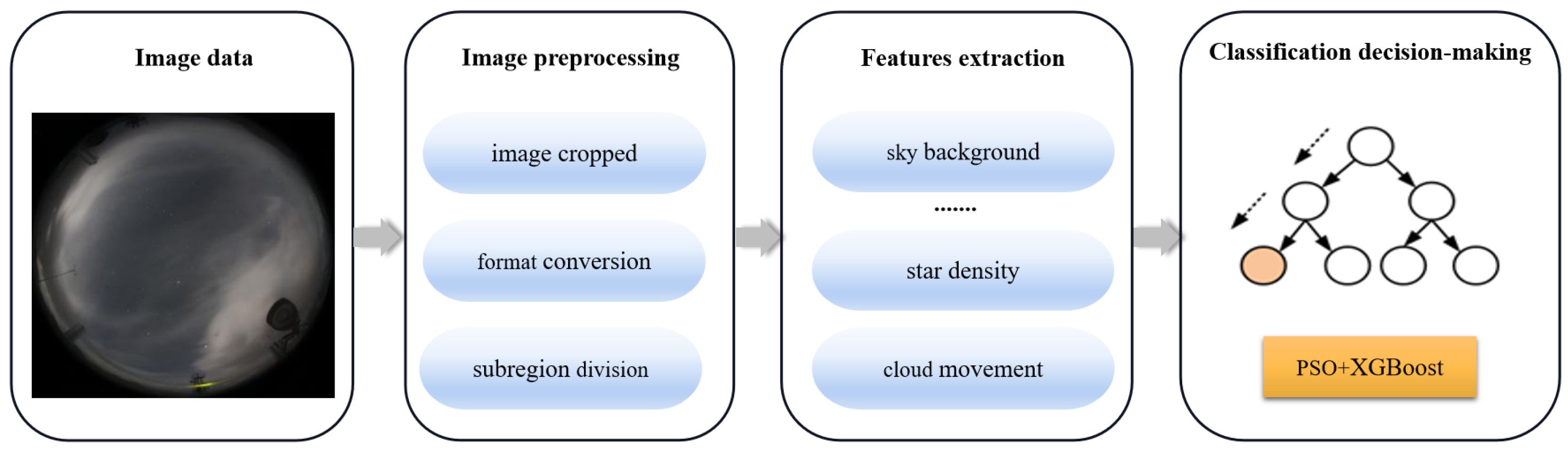
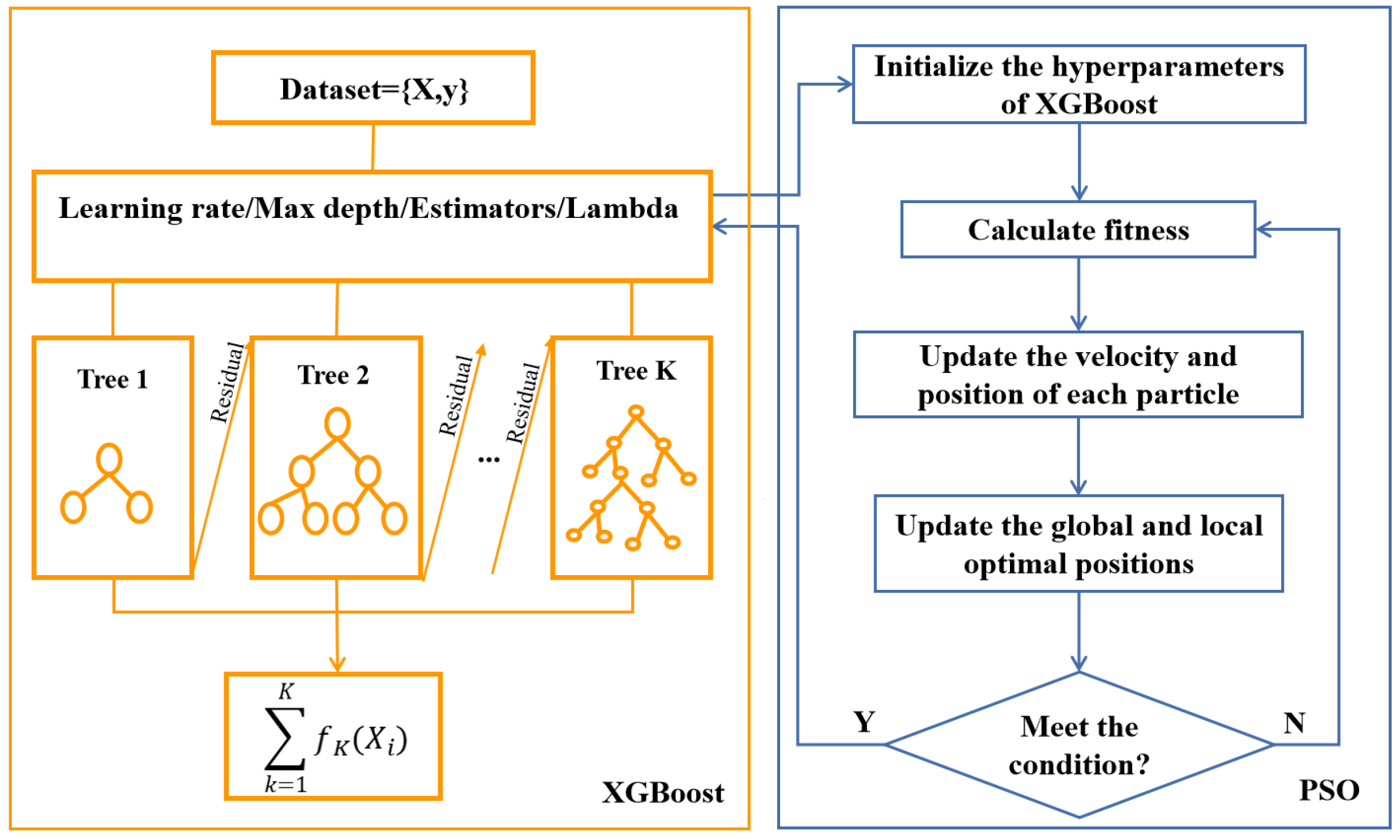
• Considering the limitations of conventional manual observation methods and the constrained computer resources of observatories, a PSO+XGBoost model is proposed to identify cloud coverage. We use the PSO algorithm to optimize the hyperparameters of XGBoost, enhancing the generalization and precision of the proposed model;
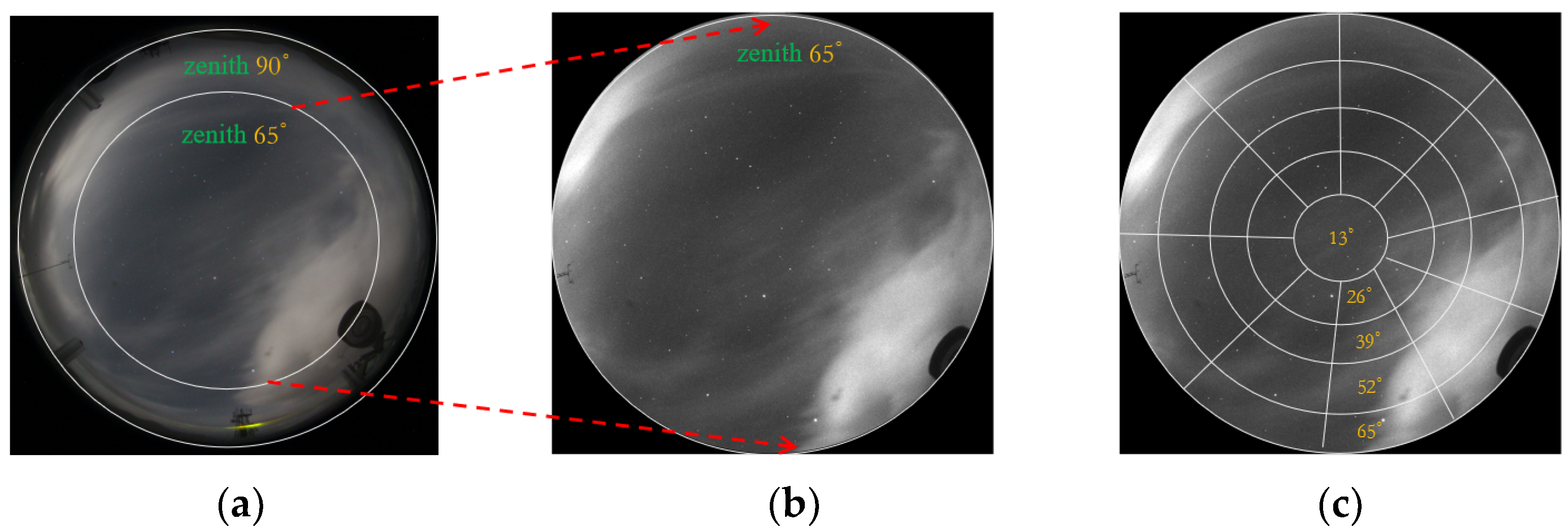
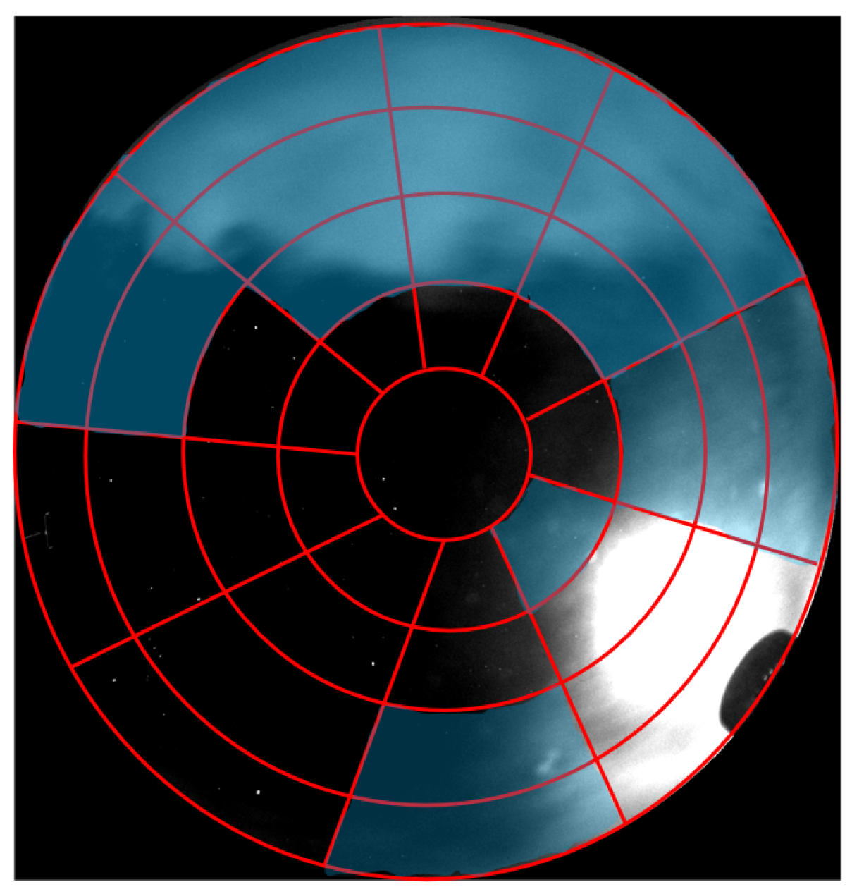
• Considering the absence of color features and poor illumination in nighttime images, one image is divided into 37 subregions, and a set of 19 features is extracted from each subregion, which improves reliability and reduces the complexity of cloud-coverage identification;
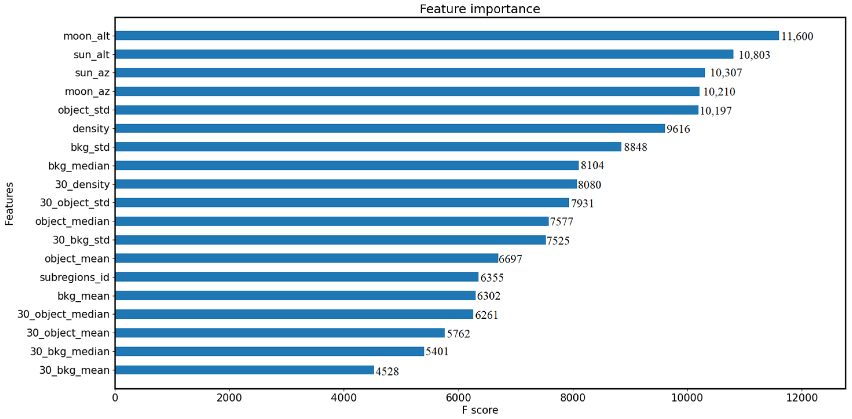
• After analyzing the relative importance of all input features, we find that the most essential feature is the elevation angle of the moon, which offers a comprehensive interpretation of nighttime image identification.

This paper is organized in the following sections. Section 2 provides a comprehensive introduction to the instrument and data description, while Section 3 provides a detailed explanation of the automated classification approach. The extensive experimental results are elaborated in Section 4. Finally, we present the conclusion in Section 5.

2. Instrument and Data Description

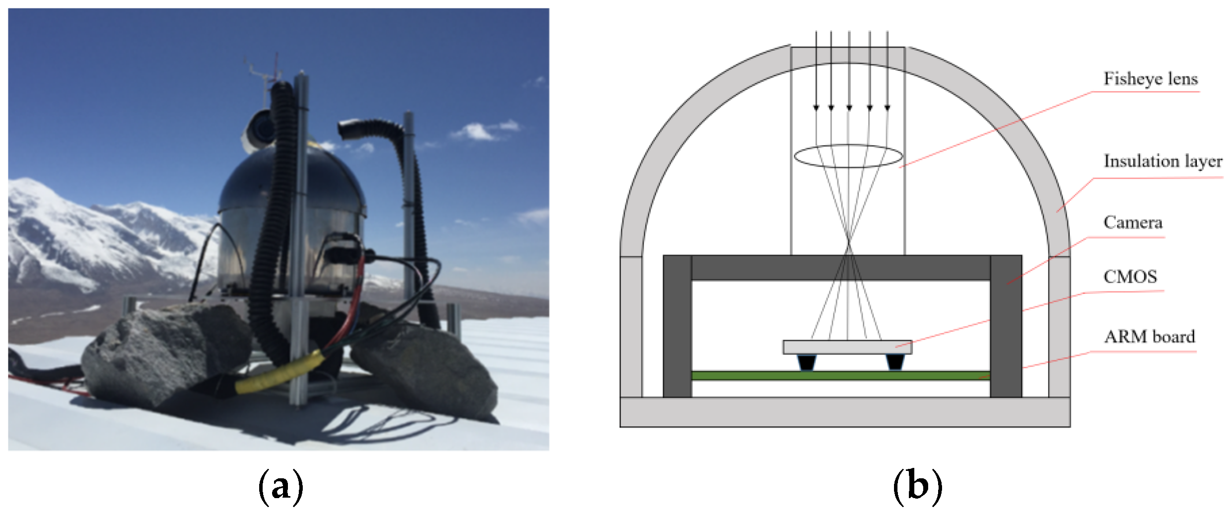
2.1. Instrument

We use the nighttime cloud images collected from KLCAM (Kunlun Cloud and Aurora Monitor). The KLCAM was built by the National Astronomical Observatories (NAO) and installed at the Muztagh Observatory (74°53′48″ E, 38°19′47″ N) in April 2017. It operated until August 2019 and 48,870 images were obtained, with an exposure time of 30 s. The KLCAM (see Figure 1a) has a 3456 × 5184 Canon EOS 100D camera (Beijing, China) and a Sigma 5 mm f/2.8 fisheye lens. KLCAM generated one image every 30 min. Figure 1b shows the structural schematic of KLCAM. A customized ARM-based computer controls the image acquisition and storage [16]. The format of raw images is RGGB. We used the two green channels as samples and merged the pixel values of the two green channels into a single channel.

To show the long-term trend within an entire year, we use nighttime images collected from KLCAM in the entire 2018 year to construct our training and testing datasets. All images are selected from when the sun’s altitude angle is below −18° [1]. Local weather conditions, such as snow, fog, and frost on the camera limit the measurement of KLCAM. Examples of fog and frost are shown in Figure 2. These defective images have been removed. In total, we have 1958 nighttime images for training and testing. We compare the available nighttime images for different months in 2018 in Figure 3. The monthly average number of nighttime images in 2018 is 163, with the lowest number of 94 in January and the highest number of 250 in November.

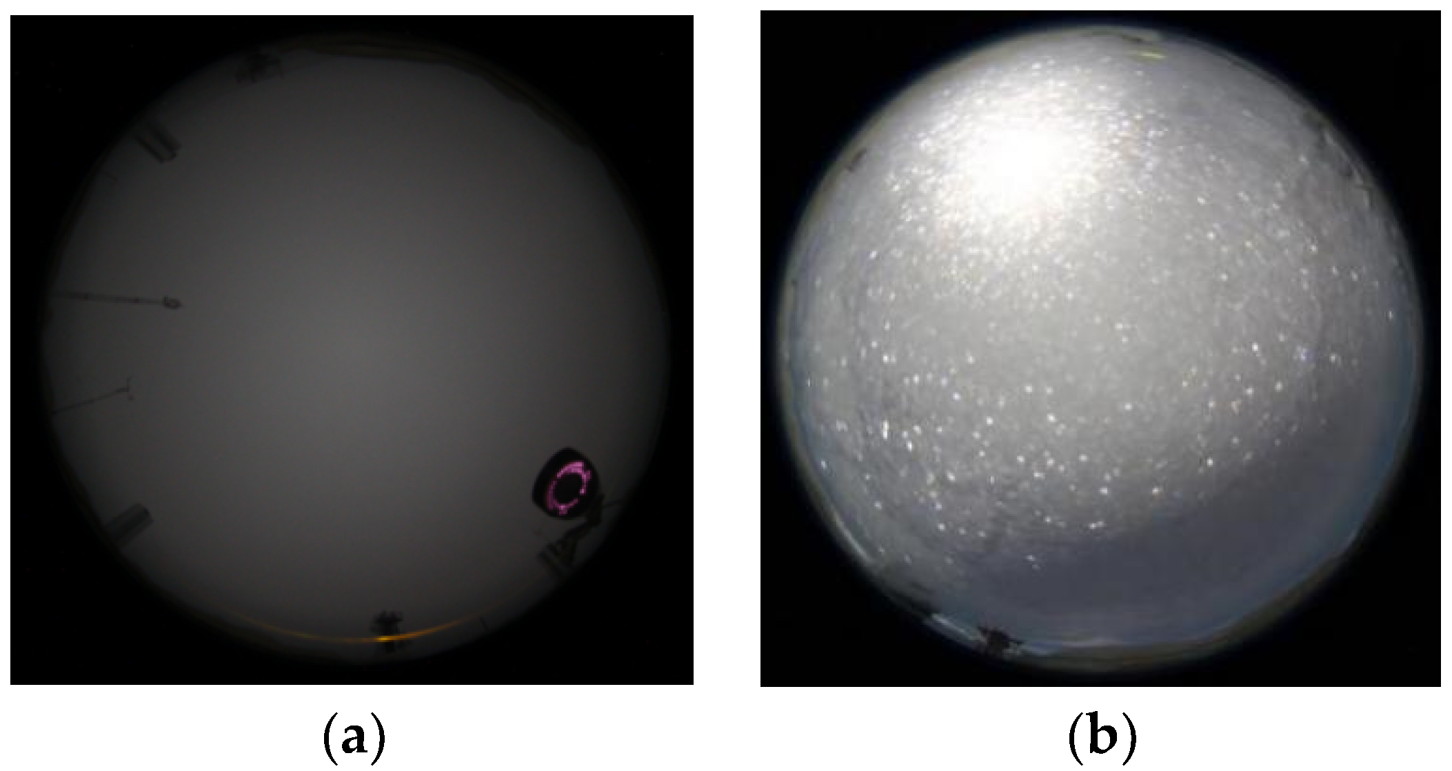
2.2. Image Preprocessing

The images contain the sky, ground buildings, and topography because of the large field of view of KLCAM. These local background features seriously impact the accuracy of cloud image recognition. Hence, we crop the images by masking the local background objects. Furthermore, we divide the images into subregions to identify the distribution of cloud coverage.

(1) Image cropping: The local background objects, such as buildings, telescopes, and topography elements, have characteristics (color or shape) similar to those of clouds. These objects may be misclassified as clouds. Furthermore, ground-based astronomical telescopes usually avoid observing objects near the horizon due to significant atmospheric interference and dispersion. Therefore, we mask the portions of the image where the zenith angle exceeds 65°. The image size after cropping is 1410 × 1430 pixels, and all images are saved in 16-bit FITS format. The cropped image is shown in Figure 4b;

(2) Subregion division: We adopted a similar method to that used for TMT site testing [3], which is widely used to classify clouds in astronomy. The TMT method divides each image into two rings centered on the local zenith. The outer ring is the area between the zenith angles of 44.7° and 65°. The inner ring is the area within the zenith angle of 44.7°. The advantage of this division is that the outer ring has the same area as the inner ring. The area outside the outer ring is ignored because of the observing limit of TMT. Our method divides each image into many subregions to get detailed spatial information. The borders of these subregions are defined in terms of zenith and azimuth. First, we divide each image into five rings centered at the local zenith, and each ring occupies the zenith angle of 13°. Then, we divide each image into 37 subregions, and the azimuth angle range of each subregion was 40°. This subregion division has the advantage that segments on the same circle have the same elevation and air mass. The labeled subregions are shown in Figure 4c.

2.3. Data-Set Description

A total of 1958 raw nighttime images are selected and further divided into 72,446 subregions. Subsequently, each subregion is labeled manually based on the cloud distribution. Each subregion is classified into three categories, as Figure 5 depicts.

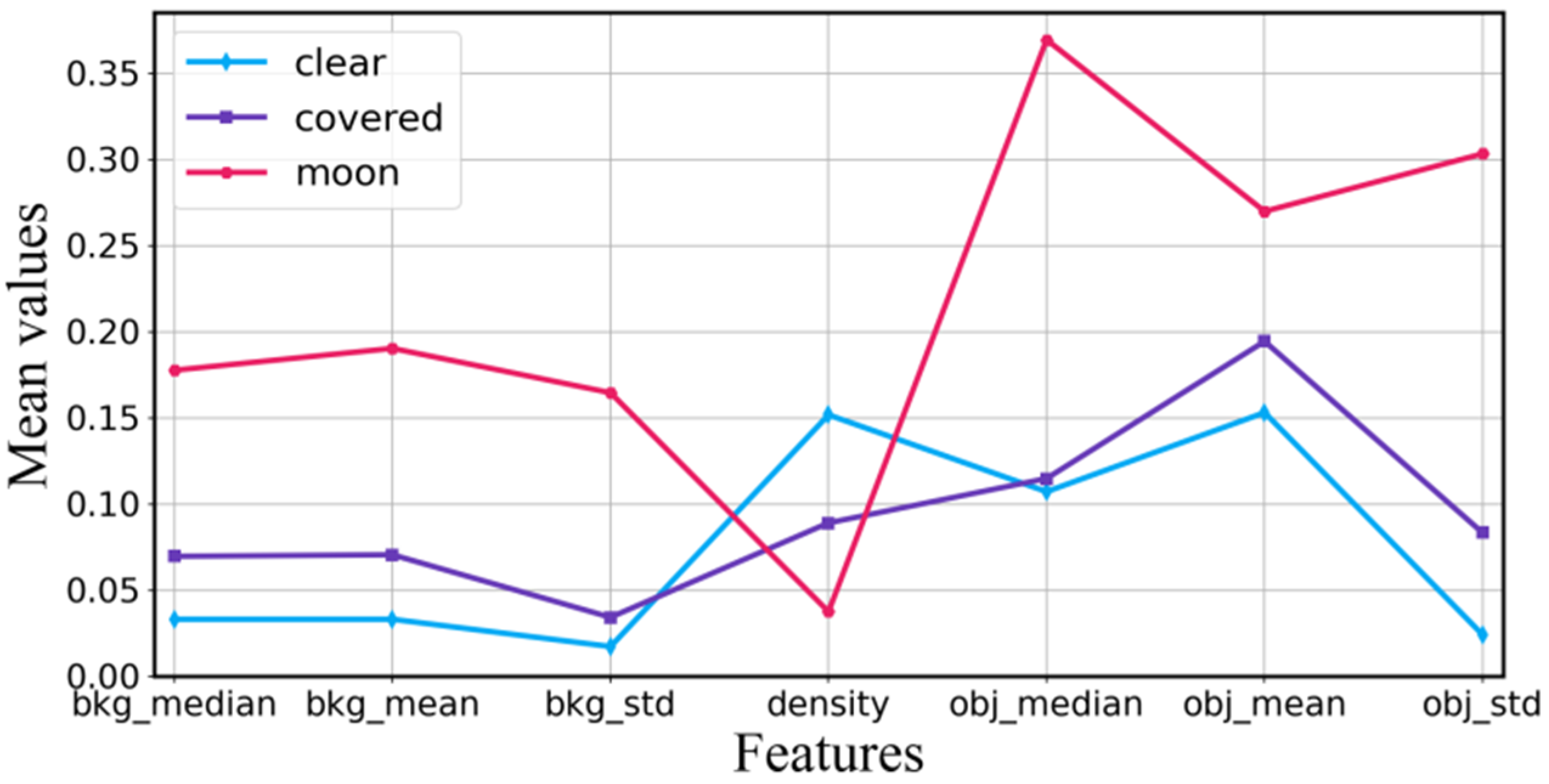
• Clear: no clouds are detected in the subregions;
• Moon: The moon’s presence distorts or obscures the edges and details of low-brightness clouds. Meanwhile, the moon significantly changes the background of the sky, making astronomical observations unimplementable. Therefore, the subregion with the moon is labeled as a “moon” category;
• Covered: all subregions that do not belong to the “clear” and “moon” categories are classified into this category.

The subregions are marked independently by three individuals to minimize the subjective assessment of a single person. Then, we follow the principle of the minority obeying the majority if the labeling results are different. This approach increases the reliability of the manual labeling method.

3. Methodology

We adopt a PSO+XGBoost model to classify nighttime cloud images automatically. The workflow of our framework is illustrated in Figure 6. Our framework comprises three components: image preprocessing, feature extraction, and classification decision-making. More specifically, image preprocessing is the premise of cloud identification. We apply feature extraction to each subregion to generate new features. These new features are inputted into the PSO+XGBoost model for cloud identification. The image preprocessing is explained in the previous section. The details of the following two components are presented in the subsequent parts of this section.

3.1. Feature Extraction

Feature extraction generates a manageable synoptic data structure from the original time-series images while preserving the characteristics of the original images as much as possible. Feature extraction can reduce the number of images and use human experience for future processing. Cloud features include visual and non-visual features related to the cloud images. We extract 19 features from the subregions to train and test our proposed model.

(1)

Sky background: The brightness of clouds depends on the conditions of the sky’s illumination. Clouds then appear as dark or bright patches against the clear sky. Furthermore, the brightness distribution of the sky background is usually uneven due to the solar or lunar elevation [17]. We utilize the sky-background estimation technique in SExtractor [18,19] to assess the gray level of the sky background of different subregions. The sky-background estimation technique uses the mode value via σ-clipping, and its formula is:

Mode = 2.5Median − 1.5Mean

(1)

(2)

Star density: The number of stars in one subregion varies significantly at different times due to the Earth’s rotation and the uneven distribution of stars. However, star density can directly reflect the clarity of the sky. For example, the presence of stars precludes the presence of thick clouds, and a high density of stars typically indicates a clear sky. Therefore, star density is utilized as a characteristic in cloud image classification. We calculate the star density by dividing the number of stars by the total subregion pixel area. This method can eliminate the variability of subregion sizes;

(3)

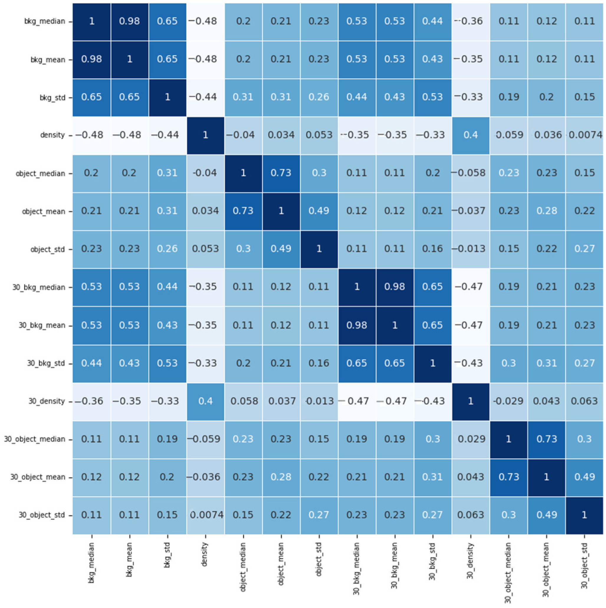
Cloud gray values: The sky and clouds have different light scattering and reflection characteristics, which induces the different gray values for the sky and clouds. Therefore, to indirectly reflect the distribution and thickness of clouds, we first calculate the gray values of each subregion and background. Then, the background’s gray values are subtracted from the gray values of each subregion to obtain the gray values of the residual image. The average, median, and standard deviation of grayscale values are calculated from residual images as features. Moreover, the gray values of subregions are also highly influenced by the elevation and azimuth angles of the moon and sun. Therefore, in addition to three grayscale features from the residual images, we extract four other features for each subregion: solar elevation angle, solar azimuth, moon elevation angle, and moon azimuth;

(4)

Cloud movement: In addition to the image’s visual characteristics, non-visual elements like the surrounding environment can influence cloud properties. Clouds are seldom stationary because the wind blows the clouds and causes clouds to move at different speeds. The dynamic behavior of clouds influences the distribution within the same subregion. Seven features have been derived from the nighttime images that were taken 30 min ago. The features include the star density, the median, mean, and standard deviation of gray values of the sky background, and the median, mean, and standard deviation of gray values of residual images.

To examine the correlation between features in current images and images from 30 min ago, we use the Kendall coefficient [20] to calculate the correlation coefficient between the features. The Kendall coefficient between variables i and j can be calculated as follows:

$${\mathrm{K}\mathrm{R}}_{\mathrm{i}\mathrm{j}}=\frac{2(\mathrm{c}-\mathrm{d})}{\mathrm{n}(\mathrm{n}-1)}$$

(2)

where c is the number of element pairs with consistency in i and j, d is the number of inconsistent element pairs, and n is the total number of samples. The value range of ${\mathrm{K}\mathrm{R}}_{\mathrm{i}\mathrm{j}}$ is between −1 and 1. When $\left|{\mathrm{K}\mathrm{R}}_{\mathrm{i}\mathrm{j}}\right|$ ≤ 0.39, it indicates a low correlation. When 0.39 ≤ $\left|{\mathrm{K}\mathrm{R}}_{\mathrm{i}\mathrm{j}}\right|$ ≤ 0.59, it indicates a moderate correlation. When $\left|{\mathrm{K}\mathrm{R}}_{\mathrm{i}\mathrm{j}}\right|$ ≥ 0.6, it indicates a high correlation.

The correlation matrix between features is shown in Figure 7; the color intensity in the figure indicates the strength of the correlation among features. Cells with more blue indicate stronger positive correlations between two features and vice versa. It can be seen that the maximum correlation coefficient between the seven features in the current images and those from 30 min ago is 0.53, which is a moderate correlation. The rest of the correlation coefficients are lower than 0.39. Hence, it can be concluded that the movement of clouds will not introduce a high correlation in features.

(5)

Subregion index: The subregion index of each subregion indicates the location of the local sky. Therefore, the subregion index is selected as a feature.

To visualize the relationships between extracted features, we plot three value curves of seven features in Figure 8. The seven features include the median, mean, and standard deviation of the sky background, star density, and residual images’ median, mean, and standard deviation. These features are normalized to a range between zero and one through the min–max normalization method. The normalization formula is as follows:

$${\mathrm{X}}_{\mathrm{n}\mathrm{o}\mathrm{r}\mathrm{m}}=\frac{\mathrm{X}-{\mathrm{X}}_{\mathrm{m}\mathrm{i}\mathrm{n}}}{{\mathrm{X}}_{\mathrm{m}\mathrm{a}\mathrm{x}}-{\mathrm{X}}_{\mathrm{m}\mathrm{i}\mathrm{n}}}$$

(3)

where X represents the original feature values, ${\mathrm{X}}_{\mathrm{n}\mathrm{o}\mathrm{r}\mathrm{m}}$ is the data matrix after normalization, and X_min and X_max represent the maximum and minimum values for each feature across all samples, respectively. And their mean values are plotted in Figure 8. It can be seen from Figure 8 that the distances for different cloud categories are significantly distinct. This means that there is a high correlation between the features and the categories of clouds. All feature values are at their highest position when the moon exists in a subregion, except for the star density. The “covered” feature curve is located between the “clear” and “moon” feature curves. When the sky is clear, the value of star density is at its highest position, while all other features show the lowest values.

3.2. PSO+XGBoost

XGBoost is a supervised algorithm based on decision trees. XGBoost utilizes ensemble learning to combine multiple decision trees to form a strong learner. This principle can solve the problem of the weak learning ability of an individual decision tree. XGBoost explicitly adds a regular term to control the complexity of the model and prevent overfitting. It constructs multiple classification and regression trees (CART) to make predictions. Each tree operates in an iterative manner, where each subsequent tree is trained to correct the errors made by the previous trees. The final prediction is the sum of the outputs of all the trees. The advantage of XGBoost is that it performs better than neural network models in processing uncorrelated tabular data.

Moreover, XGBoost has few parameters, a simple structure, and a fast training speed on the CPU. The computational capabilities are limited at actual telescope sites because most telescopes are located in remote places. Moreover, the correlation between the images is not significant. Therefore, XGBoost is suitable for image processing in these situations.

Let $D=\{X_i,y_i\}$ represent the training set with n samples, where the true value for the input sample $X_i$ is denoted by $y_i$. In cumulative training, the prediction ${\hat{\mathrm{y}}}_{\mathrm{i}}$ at step (k) can be calculated as:

$${\hat{\mathrm{y}}}_{\mathrm{i}}={\sum }_{\mathrm{k}=1}^{\mathrm{K}}{\mathrm{f}}_{\mathrm{k}}({\mathrm{X}}_{\mathrm{i}})={\hat{\mathrm{y}}}_{\mathrm{i}}^{(\mathrm{K}-1)}+f_{\mathrm{K}}({\mathrm{X}}_{\mathrm{i}})$$

(4)

where ${\hat{\mathrm{y}}}_{\mathrm{i}}^{(\mathrm{K}-1)}$ is the predicted value of the first (K − 1) trees, and $f_K(X_i)$ is the predicted model of the $K$th tree.

The objective function for regularization and optimization of the learning process is represented as:

$$obj={\sum }_{i=1}^{n}l(y_i,{\hat{y}}_i)+{\sum }_{k=1}^K\mathsf{\Omega }(f_k)$$

(5)

where $l$ is a differentiable loss function, which quantifies training error by measuring the difference between the predicted classification value (${\hat{\mathrm{y}}}_{\mathrm{i}}$) and the actual value (${\mathrm{y}}_{\mathrm{i}}$). The $\mathsf{\Omega }(f_k)$ is a regularization term that is used to prevent overfitting. The definition of the regularization term is as follows:

$$\mathsf{\Omega }(f_t)=\gamma T+\frac{1}{2}\lambda {\sum }_{j=1}^T{w}_j^2$$

(6)

where $T$ denotes the number of leaf nodes in a tree; $\gamma$ and $\lambda$ are the L1 and L2 regularization coefficients, respectively; and $w_j$ denotes the weight of the $j$th leaf node of the tree. For an in-depth exploration of XGBoost, see reference [14].

The XGBoost model includes essential hyperparameters such as the learning rate, maximum number of iterations, maximum depth, and L2 regularization term. The model’s performance profoundly depends on the expert’s experience, and the model is prone to local optimization due to the vast number of hyperparameters. To address the issue, various stochastic techniques, such as simulated annealing [21], genetic algorithm [22], and PSO [23], are employed. The PSO method possesses several benefits over other algorithms, including robust global search capability, parallel search capability, and straightforward programming implementation. Therefore, the PSO is selected to optimize the hyperparameters of XGBoost. The PSO algorithm is a heuristic methodology that draws inspiration from the collective foraging activities observed in birds. It continuously alters the movement of the whole group through sharing knowledge among group members. The target of the PSO algorithm is to ultimately realize the global optimal solution to the problem. The flowchart of PSO+XGBoost is shown in Figure 9.

4. Experimental Results and Discussion

4.1. Experimental Setup

The experiments were conducted on a customized workstation with an Intel Xeon E5-2683 v4 @ 2.10 GHz CPU, NVIDIA GeForce RTX 2080 Ti GPU, 64 GB RAM, and the Windows 10 operating system. The programming environment is Python 3.8, utilizing the integrated development environment PyCharm.

4.2. Model Parameters

We collected 72,446 labeled subregions from our 1958 training-data images. The detailed label categories are shown in

Table 1. Number of samples for different cloud types.

Types	Clear	Moon	Covered	Total
Number	47,378	2928	22,140	72,446

. We can see from Table 1 that the number of “clear” samples is 47,378, the number of “moon” samples is 2928, and the number of “covered” samples is 22,140. The ratio of “clear”, “moon”, and “covered” samples is approximately 16:1:7. This indicates that the training sample has a class imbalance, and the number of clear sky samples is in the majority compared to other categories.

To achieve better performance of the XGBoost model, we set some critical parameters of the PSO algorithm that determine the physical capacity of the network. The configurations of PSO are as follows: we use a population of 20–50 particles. The learning factors c1 and c2 increase from 1.5 to 2.0, while the weight factor w decreases from 0.9 to 0.4 in increments of 0.1. The accuracy, which is defined in Section 4.3, Equation (7), is employed as the fitness function in the PSO loop. The optimization problem is performed using PSO by iteratively adjusting the parameters of the fitness function. The optimization process stops until the number of iterations reaches the maximum of 10–30. Finally, our proposed model achieves the highest classification accuracy when the swarm’s population size is 20; learning factors c1 and c2 are 1.6 and 2, respectively; the weight factor is 0.4; and the maximum number of iterations is 25. We tuned four key hyperparameters of XGBoost by PSO, including the learning rate, the maximum tree depth, the number of iterations, and L2 regularization. Through the PSO algorithm, the four hyperparameters of XGBoost are configured as follows: the learning rate is 0.16, the maximum tree depth is 8, the number of iterations is 1200, and the L2 regularization is 4.15. To evaluate the performance of our proposed model, we have compared it with four other models: SVM, KNN, RF, and LightGBM. For a fair comparison, we fine-tuned the main hyperparameters that determine the classification performance of the comparison models with the grid search [24]. Grid search is a method that entails assessing each possible combination of hyperparameters within a predetermined range. For each set of these hyperparameters chosen, the model is recompiled, re-initialized, and retrained. Finally, these hyperparameters are configured as listed in

Table 2. Parameters of different models.

Models	SVM	KNN	RF	LightGBM	PSO+XGBoost
Parameters	kernel: RBF C: 0.1 gamma: 1 max iterations: 1200	neighbors: 7	estimators: 1200 max depth: 32	max depth: 12 estimators: 1200 learning rate: 0.02 num leaves: 32 min child samples: 20 alpha: 1 lambda: 25	learning rate: 0.16 max depth: 8 estimators: 1200 L2: 4.15

.

4.3. Evaluation Metrics

To evaluate the performance of the model on the test data, we use four evaluation metrics: accuracy, precision, recall, and F1-score. The metrics are expressed as below:

$$Accuracy=\frac{TP+TN}{TP+FP+TN+FN}$$

(7)

$$Precision=\frac{TP}{TP+FP}$$

(8)

$$Recall=\frac{TP}{TP+FN}$$

(9)

$$F1\text{-}score=\frac{2\times Precision\times Recall}{Precision+Recall}$$

(10)

where FP is the number of false-positive instances. TN is the number of true-negative instances. TP is the number of true-positive instances. FN is the number of false-negative instances.

4.4. Experimental Results

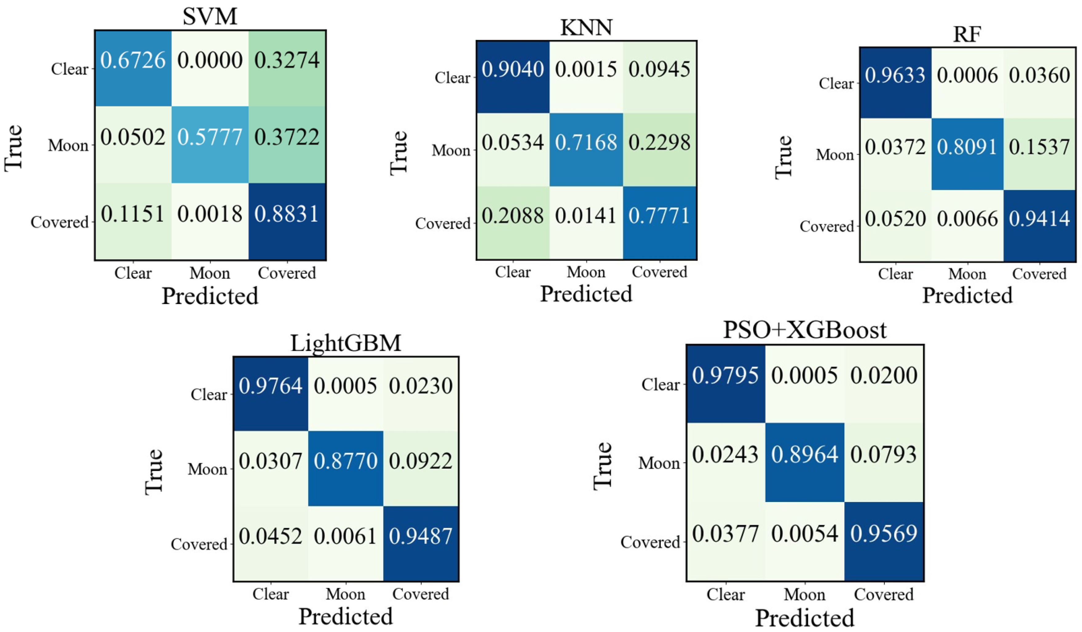
4.4.1. Comparison of Different Models

In this study, 72,446 samples are randomly allocated into training and testing sets in a ratio of 8:2.

Table 3. Classification results of different models (%) and classification time for one image (s).

Class		Clear	Moon	Covered	Average Accuracy	Time (s)
SVM	Precision	99.21	97.81	53.89	73.26	2.492
	Recall	67.26	57.77	88.31
	F1 score	77.78	72.63	66.94
KNN	Precision	89.98	85.36	76.75	85.74	2.547
	Recall	90.40	71.68	77.71
	F1 score	90.19	77.92	77.23
RF	Precision	97.31	93.46	90.49	95.01	2.122
	Recall	96.33	80.91	94.14
	F1 score	96.82	86.73	92.28
LightGBM	Precision	97.70	94.43	93.83	96.38	1.279
	Recall	97.64	87.70	94.87
	F1 score	97.70	90.94	94.35
PSO+XGBoost	Precision	98.09	95.03	94.66	96.91	0.975
	Recall	97.95	89.64	95.69
	F1 score	98.02	92.26	95.17

displays the classification results for various cloud categories and the classification time for one cloud image. The classification accuracy of the PSO+XGBoost model reached 96.91%, surpassing SVM, KNN, RF, and LightGBM by 23.65%, 11.17%, 1.90%, and 0.53%, respectively. In addition, the PSO+XGBoost model exhibited superior precision, recall, and F1 score in the “clear”, “moon”, and “covered” categories. These results validate that our proposed model has remarkable performance in classification recognition in terms of accuracy and stability. In addition, the classification time of our proposed model for one cloud image is 0.975 s. The classification time can meet the demands of real-time telescope scheduling.

Since the accuracy of PSO+XGBoost and LightGBM is similar, we use an independent sample t-test to assess the statistical significance between these two models. The test significance level (α) is set at 0.05, and the original hypothesis (H0) posits no substantial disparity in accuracy. If the p-value is less than 0.05, the two models are regarded as significant differences. If the p-value is greater than or equal to 0.05, the two models are considered not statistically different. The independent sample t-test results between PSO+XGBoost and LightGBM are illustrated in

Table 4. Independent sample t-test for two models.

Models	Accuracy	t-Value	p-Value
PSO+XGBoost	0.9691	3.748	0.006
LightGBM	0.9638

. As can be seen, the p-value is 0.006, which is less than 0.05, indicating a significant statistical difference.

To evaluate the classification results more intuitively, a confusion matrix is used to express the relationship between the classification result and the true label. The corresponding result is depicted in Figure 10. The horizontal axis of the confusion matrix represents the predicted labels of the cloud image samples, while the vertical axis represents the true labels. The main diagonal elements represent the correct classification results. The variation in color tones in the confusion matrix reflects the ratio of predicted labels to true labels. The color tones change from blue to green. The darker blue indicates a higher ratio of predicted labels to true labels. The color changes to green and even white as the ratio decreases. As shown in Figure 10, the classification accuracy of PSO+XGBoost for the “clear” class is 97.95%, which is higher than SVM, KNN, and RF by 30.69%, 7.55%, and 1.62%, respectively, and higher than LightGBM, as reported in paper [13] by 0.31%. The classification accuracies for the “moon” and “covered” samples are 89.64% and 95.69%, respectively. Therefore, PSO+XGBoost has the best performance among all models. In the PSO+XGBoost confusion matrix, the class with the highest probability of misclassification is the “moon” class. Specifically, there is a 7.93% likelihood that the “moon” class is misclassified as the “covered” class. The main reason is that the moon in some cloud images is small, which causes their grayscale values to be similar to those of the “covered” class. Furthermore, the grayscale values of the brighter clouds at night are similar to those of the moon. The misclassification ratio from “covered” to “clear” is 3.77%. This misclassification is primarily attributed to poor illumination conditions in nighttime cloud images and the low gray value of the images. These factors result in similar grayscale values for both categories of image samples.

For model comparison, we have assessed the computational complexity of RF, LightGBM, and PSO+XGBoost, respectively, because these three models are decision-tree-based supervised methods.

The model complexity is defined as follows:

$$C_{model}=T\times n\times d\times m+T\times m$$

(11)

where T is the number of trees, n is the number of training samples, d is the feature dimensions, and m is the maximum depth of each tree. The model complexity is the sum of the training and prediction stages. According to Table 2, the model complexity of the RF is 42,284,736,000, the model complexity of the LightGBM is 15,856,776,000, and the model complexity of the PSO+XGBoost is 10,571,184,000, respectively. From these results, we can see that the PSO+XGBoost has the lowest model complexity. Therefore, the classification results are convincing. We do not calculate the model complexity of SVM and KNN, because the SVM and KNN are not decision-tree-based supervised methods.

To analyze the relative importance of the input features, we calculated the number of times each feature appears in all decision trees and plotted the results in Figure 11. The more times a feature is used to construct a decision tree, the more important it is. As shown in Figure 11, it is clear that the elevation angle of the moon has the highest importance score in the cloud-distribution classification. The reason is that when the moon is present, the edges and details of low-luminosity clouds become blurred and difficult to observe. Furthermore, the moon’s brightness severely changes the background of the sky, reducing the observable magnitude and making astronomical observations unimplementable.

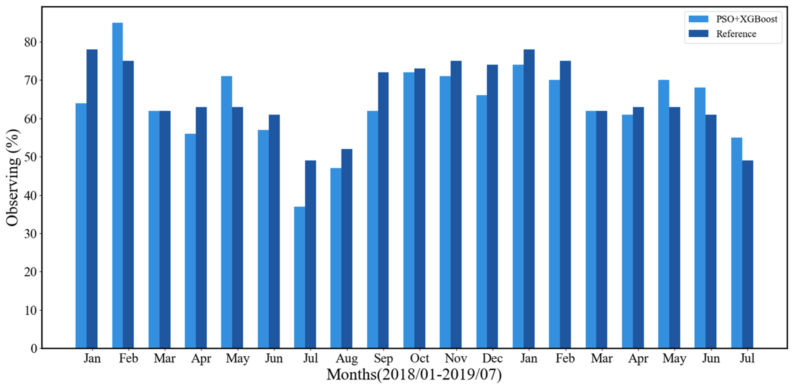
4.4.2. Comparative Results of the Manual Observation Technique

To evaluate our proposed model’s accuracy and generalization ability, we compared the results with the manual observation at Muztagh [25]. The manual observation was used to analyze nighttime cloud images from 2017 to 2021 to determine the length of observable time. The specific method divides the nighttime images into two regions within zenith angles of 65°, with the outer region at a zenith angle of 65° and the inner region at 44.7°. The outer and inner circles without clouds are considered “clear”. The term “outer” indicates that clouds are only detected inside the outer ring (between 65° and 44.7° circles). The observable time is the sum of “clear” and “outer”. Based on manual observation, the percentage of observable time at Muztagh in 2018 is 66%.

To align the evaluation criteria with the manual observation as closely as possible, we segment the nighttime cloud images into inner and outer circles delineated by zenith angles of 39°. The zenith angles for manual observation and our proposed method are 44.7° and 39°, respectively. The difference between the zenith angles of the inner circle of the two methods is 5.7°. To ensure the reliability of the comparison results, the definitions of cloud distribution and observable time are identical for both methods. Figure 12 displays example images of the “clear” and “outer” cloud categories in this paper.

Figure 13 shows the monthly observable time of the manual observation method and the proposed method from January 2018 to July 2019. Compared with the manual observation method, the monthly average error of the proposed method was 7% in 2018, while it was 4.4% in 2019. The maximum error of the proposed method occurred in January 2018, with an error of 14%. The main reason is that the number of available images is small due to underexposed nighttime images. The proposed method achieves 63% of the observable time throughout the entire year of 2018, which is less than 3% of the observable time evaluated by manual observation. The main reason for this error is that we use an all-sky camera with a 30 min sampling period. The lower sampling rate may lead to variations in cloud-cover distribution between consecutive images, and some of the cloud-cover distribution information may be missing. In contrast, the sampling period in the manual observation method is 5 min, which can capture more detailed information on cloud distribution.

To make a fair comparison as much as possible, we segmented the nighttime cloud images into two regions through one circle at the zenith angle of 52°, as shown in Figure 14. We calculated the full-year observable time in 2018 through our proposed method. The observable time is 64% within the 52° zenith-angle circle, while the observable time is 63% within the 39° zenith-angle circle. We can see that the difference in observable time between 52° and 39° zenith angles is only 1%. Therefore, we can infer that the error of observable time between 44.7° and 39° zenith angles is less than 1%.

5. Conclusions

Cloud coverage directly impacts the quality and efficiency of telescope observations. Traditional manual cloud observation methods are subjective and labor intensive. Therefore, this paper proposed an automatic cloud identification method using PSO+XGBoost. The technique utilized the all-sky camera nighttime cloud images in Muztagh in 2018. We divided nighttime cloud images into 37 subregions. Each subregion was labeled as “clear”, “moon”, or “covered” based on the cloud distribution. The experimental results showed that the overall classification accuracy of the PSO+XGBoost method reached 96.91%. The precision, recall, and F1 scores outperformed other machine-learning algorithms, such as SVM, KNN, RF, and LightGBM. The results were compared with the manual observation method to verify the accuracy and generalization ability of the model. The comparison results revealed that the average error in the monthly observable time in 2018 was 7%. These results indicated that the proposed method met the observation requirements. The classification time of our proposed method for one cloud image was 0.975 s. This time met the real-time requirements of the telescope scheduling program.

Nevertheless, our proposed method had the following weaknesses: (1) The proposed method can only roughly locate sky areas without cloud and moonlight contamination. In the future, we need to calibrate the positions of objects in images. This will allow us to determine cloud distribution accurately through projection and curve fitting. We may improve the positional accuracy of cloud identification and enable a better schedule for the telescope; (2) Most of the features extracted in this study were based on the grayscale values of the images. Therefore, additional features may be considered in future studies to conduct a more comprehensive understanding of cloud characteristics. These features may include meteorological data, which can influence cloud movement and formation. Moreover, the spectrum can be considered as part of the features. The spectrum reflects the physical attributes of the cloud, such as brightness, whiteness, and temperature.

References

1. Zou, H.; Zhou, X.; Jiang, Z.; Ashley, M.C.B.; Cui, X.; Feng, L.; Gong, X.; Hu, J.; Kulesa, C.A.; Lawrence, J.S. Sky brightness and transparency in THEI-BAND at dome a, antarctica. Astron. J. 2010, 140, 602–611. [Google Scholar] [CrossRef]
2. Lawrence, J.S.; Ashley, M.C.B.; Tokovinin, A.; Travouillon, T. Exceptional Astronomical Seeing Conditions above Dome C in Antarctica. Nature 2004, 431, 278–281. [Google Scholar] [CrossRef] [PubMed]
3. Skidmore, W.; Schöck, M.; Magnier, E.; Walker, D.; Feldman, D.; Riddle, R.; Els, S.; Travouillon, T.; Bustos, E.; Seguel, J.; et al. Using All Sky Cameras to Determine Cloud Statistics for the Thirty Meter Telescope Candidate Sites. Proc. SPIE 2008, 7012, 701224. [Google Scholar]
4. Cao, Z.H.; Hao, J.X.; Feng, L.; Jones, H.R.A.; Li, J.; Xu, J.; Liu, L.Y.; Song, T.F.; Wang, J.F.; Chen, H.L. Data Processing and Data Products from 2017 to 2019 Campaign of Astronomical Site Testing at Ali, Daocheng and Muztagh-Ata. Res. Astron. Astrophys. 2020, 20, 082–0104. [Google Scholar] [CrossRef]
5. Yang, X.; Shang, Z.H.; Hu, K.L.; Hu, Y.; Ma, B.; Wang, Y.J.; Cao, Z.H.; Ashley, M.C.B.; Wang, W. Cloud Cover and Aurora Contamination at Dome A in 2017 from KLCAM. Mon. Not. R. Astron. Soc. 2020, 501, 3614–3620. [Google Scholar] [CrossRef]
6. Dev, S.; Savoy, F.M.; Lee, Y.-H.; Winkler, S. Nighttime Sky/Cloud Image Segmentation. In Proceedings of the 2017 IEEE International Conference on Image Processing (ICIP), Beijing, China, 17–20 September 2017; 2017; 2017, pp. 345–349. [Google Scholar]
7. Afiq, M.; Hamid, A.; Mohd, W.; Mohamad, N.S. Urban Night Sky Conditions Determination Method Based on a Low Resolution All-Sky Images. IEEE Conf. Proc. 2019, 2019, 158–162. [Google Scholar]
8. Jadhav, T.; Aditi, K. Cloud Detection in All Sky ConCam Images by Gaussian Fitting and Valley Detection in Histogram. In Proceedings of the 2015 Eighth International Conference on Contemporary Computing (IC3), Noida, India, 20–22 August 2015; pp. 275–278. [Google Scholar]
9. Yin, J.; Yao, Y.Q.; Liu, L.Y.; Qian, X.; Wang, H.S. Cloud Cover Measurement from All-Sky Nighttime Images. J. Phys. Conf. Ser. 2015, 595, 012040–012045. [Google Scholar] [CrossRef]
10. Mandát, D.; Pech, M.; Ebr, J.; Miroslav, H.; Prouza, M.; Bulik, T.; Ingomar, A. All Sky Cameras for the Characterization of the Cherenkov Telescope Array Candidate Sites. arXiv 2013, arXiv:1307.3880. [Google Scholar]
11. Shi, C.J.; Zhou, Y.T.; Qiu, B.; Guo, D.J.; Li, M.C. CloudU-Net: A Deep Convolutional Neural Network Architecture for Daytime and Nighttime Cloud Images’ Segmentation. IEEE Geosci. Remote Sens. Lett. 2021, 18, 1688–1692. [Google Scholar] [CrossRef]
12. Li, X.T.; Wang, B.Z.; Qiu, B.; Wu, C. An All-Sky Camera Image Classification Method Using Cloud Cover Features. Atmos. Meas. Tech. 2022, 15, 3629–3639. [Google Scholar] [CrossRef]
13. Mommert, M. Cloud Identification from All-Sky Camera Data with Machine Learning. Astron. J. 2020, 159, 178–185. [Google Scholar] [CrossRef]
14. Chen, T.Q.; Guestrin, Q. XGBoost: A Scalable Tree Boosting System. CoRR 2016, 2016, 785–794. [Google Scholar]
15. Jin, Q.W.; Fan, X.T.; Liu, J.; Xue, Z.X.; Jian, H.D. Estimating Tropical Cyclone Intensity in the South China Sea Using the XGBoost Model and FengYun Satellite Images. Atmosphere 2020, 11, 423–445. [Google Scholar] [CrossRef]
16. Shang, Z.H.; Hu, K.L.; Yang, X.; Hu, Y.; Ma, B.; Wang, W. Kunlun Cloud and Aurora Monitor. Proc. SPIE Astron. Telesc. Instrum. 2018, 10700, 1070057. [Google Scholar]
17. Yang, J.; Min, Q.L.; Lu, W.T.; Ma, Y.; Yao, W.; Lu, T.S.; Du, J.; Liu, G.Y. A Total Sky Cloud Detection Method Using Real Clear Sky Background. Atmos. Meas. Tech. 2016, 9, 587–597. [Google Scholar] [CrossRef]
18. Bertin, E.; Arnouts, S. SExtractor: Software for Source Extraction. Astron. Astrophys. Suppl. Ser. 1996, 117, 393–404. [Google Scholar] [CrossRef]
19. Annunziatella, M.; Mercurio, A.; Brescia, M.; Cavuoti, S.; Longo, G. Inside Catalogs: A Comparison of Source Extraction Software. Publ. Astron. Soc. Pac. 2013, 125, 68–82. [Google Scholar] [CrossRef]
20. Du, M.S.; Wei, Y.X.; Hu, Y.P.; Zheng, X.W.; Ji, C. Multivariate Time Series Classification Based on Fusion Features. Expert Syst. Appl. 2024, 248, 123452–123465. [Google Scholar] [CrossRef]
21. Liu, S.C.; Luo, Y. Square-Based Black-Box Adversarial Attack on Time Series Classification Using Simulated Annealing and Post-Processing-Based Defense. Electronics 2024, 13, 650–663. [Google Scholar] [CrossRef]
22. Diaz, A.; Darin, J.M.; Edwin, R.T. Optimization of Topological Reconfiguration in Electric Power Systems Using Genetic Algorithm and Nonlinear Programming with Discontinuous Derivatives. Electronics 2024, 13, 616–638. [Google Scholar] [CrossRef]
23. Zhang, J.Y.; Chen, K.J. Research on Carbon Asset Trading Strategy Based on PSO-VMD and Deep Reinforcement Learning. J. Clean. Prod. 2023, 140322–140337. [Google Scholar] [CrossRef]
24. Belete, D.M.; Huchaiah, M.D. Grid search in hyperparameter optimization of machine learning models for prediction of HIV/AIDS test results. Int. J. Comput. Appl. 2022, 44, 875–886. [Google Scholar] [CrossRef]
25. Xu, J.; Feng, G.J.; Pu, G.X.; Wang, L.T.; Cao, Z.H.; Ren, L.Q.; Zhang, X.; Ma, S.G.; Bai, C.H.; Esamdin, A. Site-Testing at the Muztagh-Ata Site V. Nighttime Cloud Amount during the Last Five Years. Res. Astron. Astrophys. 2023, 23, 045015. [Google Scholar]
Figure 1. (a) KLCAM at Muztagh site; (b) structural schematic of KLCAM.
Electronics 13 01503 g001
Figure 2. Examples of nighttime cloud images which are limited by local weather conditions. (a) fog; (b) frost.
Electronics 13 01503 g002
Figure 3. Monthly available nighttime images in 2018.
Electronics 13 01503 g003
Figure 4. Process of image preprocessing. (a) Raw image; (b) image after cropping and format conversion; (c) divided and labeled subregions.
Electronics 13 01503 g004
Figure 5. Example of KLCAM nighttime image classification definition. Black represents the subregions without clouds, light blue represents the presence of clouds in subregions, and bright white is the moon.
Electronics 13 01503 g005
Figure 6. Flow chart of an automatic classification system for nighttime cloud images.
Electronics 13 01503 g006
Figure 7. Correlation matrix between features.
Electronics 13 01503 g007
Figure 8. Comparison of different features.
Electronics 13 01503 g008
Figure 9. Flow chart of PSO+XGBoost.
Electronics 13 01503 g009
Figure 10. Confusion matrix of different models.
Electronics 13 01503 g010
Figure 11. Feature importance scores.
Electronics 13 01503 g011
Figure 12. Example images of “clear” and “outer” cloud categories with the inner 39° circle at Muztagh. (a) clear, (b) outer.
Electronics 13 01503 g012
Figure 13. Comparison of PSO+XGBoost algorithm and manual observation method [25].
Electronics 13 01503 g013
Figure 14. Example images of “clear” and “outer” cloud categories with the inner 52° circle at Muztagh. (a) clear, (b) outer.
Electronics 13 01503 g014