

Several Approaches for the Prediction of the Operating Modes of a Wind Turbine


Abstract
:1. Introduction
1.1. Background and Previous Works
1.2. Forecasting Problem
1.3. Main Contributions and the Organization of the Paper
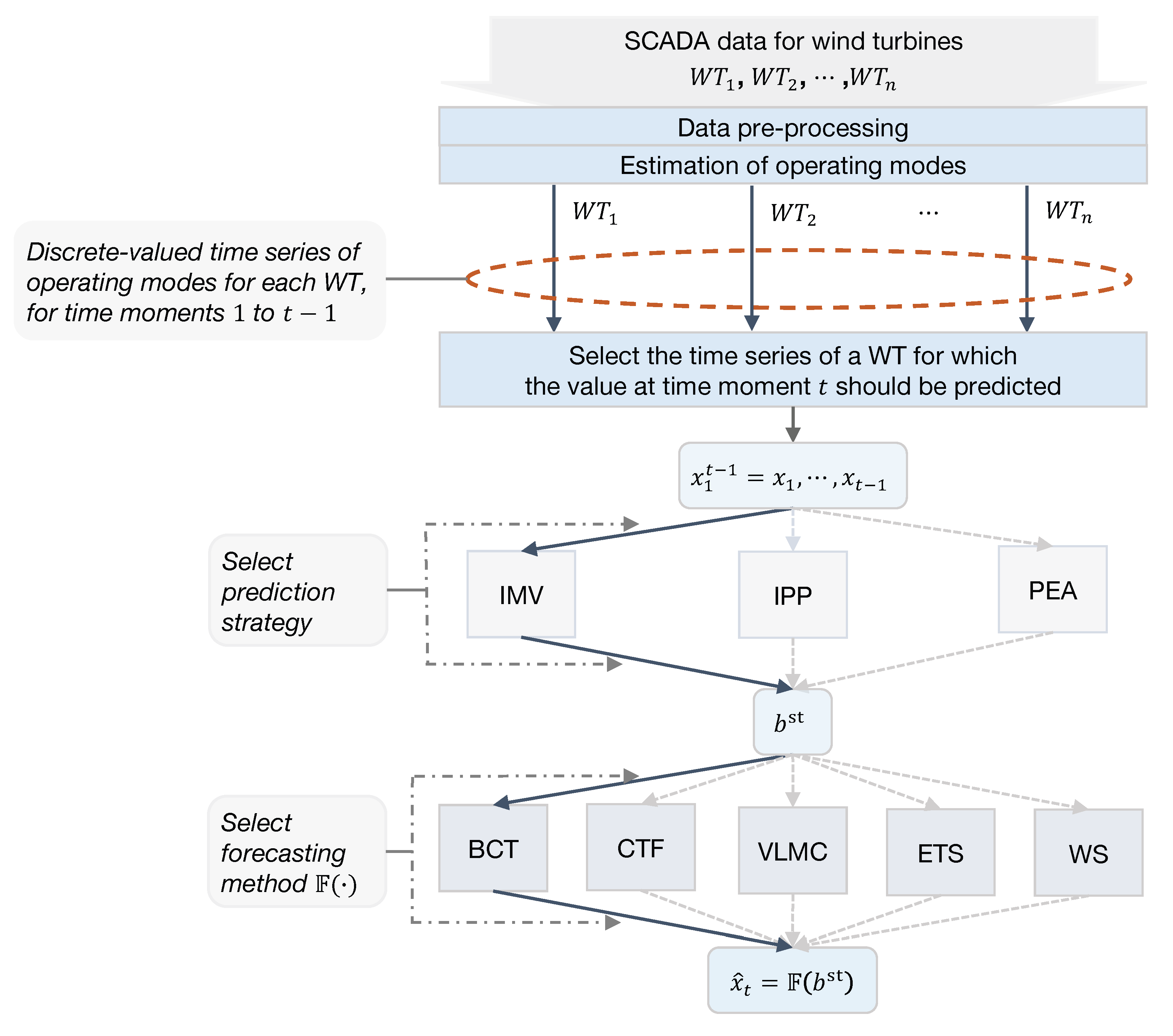
- To circumvent the difficulties related to missing data, we define three prediction strategies, which are dubbed as follows: ignore missing values (IMV), imputation and prediction (IPP), and prediction with extended alphabet (PEA). The main difference between strategies consists in the way in which they use the past samples of a discrete-valued time series with missing values for predicting the value of . In practice, each strategy selects in a different manner the most relevant samples from the past that should be used in the forecasting of and stores them in the buffer . The length of the buffer is the same for all strategies, but the data stored in the buffer are different.
- These strategies are applied in conjunction with five different forecasting methods (BCT, VLMC, CTF, ETS, WS) in experiments conducted on two datasets. If we suppose that the operator stands for the forecasting method that we apply, then the predicted value is . For clarity, we provide in Figure 1 a graphical representation of the steps that are needed for finding the predicted operating mode for a particular turbine starting from the SCADA data available for the turbines in the wind farm.
- The comparison of the prediction results allows us to draw conclusions on the prediction accuracy and computational burden for each pair strategy/method.
2. Materials and Methods
2.1. Data
2.2. Data Pre-Processing
- (i)
- Eliminating similar parameters: (1) A variable may be represented by various attributes. For example, the wind speed variable encompasses its mean, maximum, minimum, and standard deviation. We discard parameters that do not align with our purpose of the analysis, which is forecasting operating modes. Consequently, we retain only the mean value; (2) Multiple sensors monitor the same variable. For example, two anemometers are installed on the nacelle of a wind turbine to monitor the wind speed. In this case, we use the average value of the two anemometers, which is also given in the dataset; (3) Within a wind turbine, certain variables, like generator converter speed, generator speed, and rotor speed, are interconnected. Including all these parameters can lead to over-fitting, so one variable from each group of similar data is chosen when estimating the operating modes. A point to note is that the ‘torque’ variable is absent in the Kelmarsh wind farm dataset. To rectify this, we generate the values for the torque variable, T, using power P and rotor speed (expressed in radians/s), with the following formula: [14]. This ensures consistent comparisons across datasets.
- (ii)
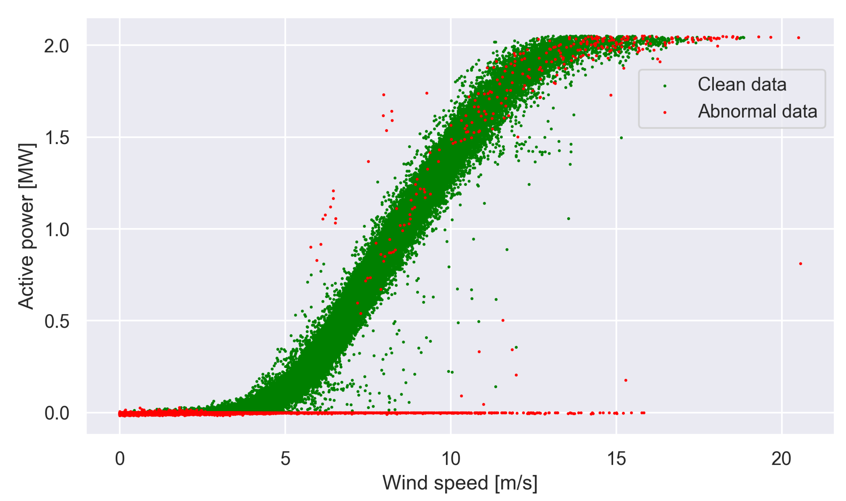
- Removal of measurements deemed outliers: The data are anticipated to exhibit a range of irregularities because these datasets have been automatically recorded by the system. These irregularities can adversely affect the accuracy of operating mode estimations. Therefore, procedures are applied to eliminate measurements deemed to be outliers. More precisely, the following procedures are applied to each wind turbine individually: (1) Exclude data entries that show negative active power values as these indicate times when the turbine is not in operation; (2) Remove data points that exhibit substantial deviation from a two-dimensional binning of wind speed and wind direction. Firstly, a point is discarded if a bin contains only one point. Secondly, remove data points that exhibit substantial deviation from the anticipated active power. The effect of removing these measurements is illustrated in Figure 2.
- (iii)
- Data standardization: The dataset records are a combination of angular and nonangular variables; thus, this diversity complicates the analysis. Angular variables in the dataset, like blade angle and wind direction, need to be converted by applying the sine and cosine transforms to become nonangular. Moreover, we normalize the selected parameters such that they are scaled between 0 and 1.
- La Haute Borne farm: generator bearing 1 temperature, generator bearing 2 temperature, pitch angle (sine), pitch angle (cosine), torque, rotor bearing temperature, gearbox oil sump temperature, gearbox inlet temperature, gearbox bearing 1 temperature, gearbox 2 temperature, generator stator temperature, generator speed.
- Kelmarsh farm: front bearing temperature, rear bearing temperature, gear oil inlet temperature, generator bearing front temperature, generator bearing rear temperature, gear oil temperature, stator temperature 1, torque, rotor bearing temp, generator RPM, blade angle (sine), blade angle (cosine).
2.3. Operating Modes
2.4. Prediction Strategies
- (i)
- Ignore Missing Values (IMV): The first strategy is the most straightforward and consists of producing a new time series by discarding from all the occurrences of the symbol . Let be the length of the resulting time series and let be the operator defined in Section 1.3. For each t in the set , we obtain without difficulties . It is clear that contains measurements collected before the last 24 h whenever the set of measurements from the last 24 h is not complete. This approach simplifies the prediction process as it only focuses on available data.
- (ii)
- Imputation and Prediction (IPP): In this strategy, we impute the missing values as follows. For each , we compute , which is guaranteed to be a symbol from . If , then we replace in the time series the symbol with the estimate . Apart from the particular case when , this will have an important effect on the predicted values because the imputed symbol will be employed in the calculations involved by the application of the operator .
- (iii)
- Prediction with Extended Alphabet (PEA): The last strategy addresses missing values by treating them as an additional mode, so the symbol is recognized as a distinct mode within the predictive framework. As a result, the time series is not altered during the prediction process, which is different from IPP. Remark that for both IPP and PEA, the number of time points for which the predictions are produced is the same: . For each such time point, the operating mode predicted by PEA can potentially be (which is not possible for IMV and IPP). This can be regarded as a capability of PEA to anticipate scenarios where the next observation may not be recorded or exhibit significant deviations from the standard operation of a wind turbine. We do not adopt this viewpoint in our work. Because of that, we use PEA only for the prediction of valid entries of the time series.
| Algorithm 1: Evaluation of accuracy for various prediction strategies |
Input: [discrete-valued univariate time series], [ and is complete], [operator forecasting method] Initialisation:, , for , , for fordo if is a missing value then else for do end for for do if then end if end for end if end for fordo end for Output: , and |
2.5. Forecasting Methods
2.5.1. Bayesian Context Tree (BCT)
2.5.2. Conditional Tensor Factorization (CTF)
2.5.3. Variable-Length Markov Chains (VLMC)
2.5.4. Exponential Smoothing (ETS)
2.5.5. Whittaker Smoother (WS)
3. Experimental Results
3.1. Preamble
3.2. BCT
3.3. Comparison between BCT and CTF
3.4. Comparison between BCT and Other Forecasting Methods
3.4.1. Comparison with VLMC
3.4.2. Comparison with ETS
3.4.3. Comparison with WS
4. Conclusions, Limitations, and Future Research
Author Contributions
Funding
Data Availability Statement
Acknowledgments
Conflicts of Interest
Abbreviations
| CA | context algorithm |
| CTW | context tree weighting |
| LASSO | least absolute shrinkage and selection operator |
| IMV | ignoring missing values |
| IPP | imputation and prediction |
| PEA | prediction with extended alphabet |
| BCT | Bayesian context tree |
| MAP | maximum a posteriori |
| VLMC | variable-length Markov chains |
| CTF | conditional tensor factorization |
| ETS | exponential smoother |
| WS | Whittaker smoother |
Appendix A

| Forecasting Method | User-Selected Option | Values Used in Experiments |
|---|---|---|
| BCT | Maximum memory length (D) | 5 |
| CTF | Maximum order Markov model (D) | 10 |
| Number of iterations MCMC | 5000 | |
| for posterior computation | (initial burn-in 1000) | |
| VLMC | Threshold used in pruning () | Quantile function of |
| ETS | ETS model | Simple exponential smoother with an additive error (ANN) |
| WS | Order of differences (m) | 3 |
| Range smoothing parameter () | g take values on a uniform grid on , | |
| grid step |
| Wind Farm | Forecasting Method | Turbine | IMV | IPP Accuracy (%) | PEA Accuracy (%) | |
|---|---|---|---|---|---|---|
| Accuracy (%) | Time (min) | |||||
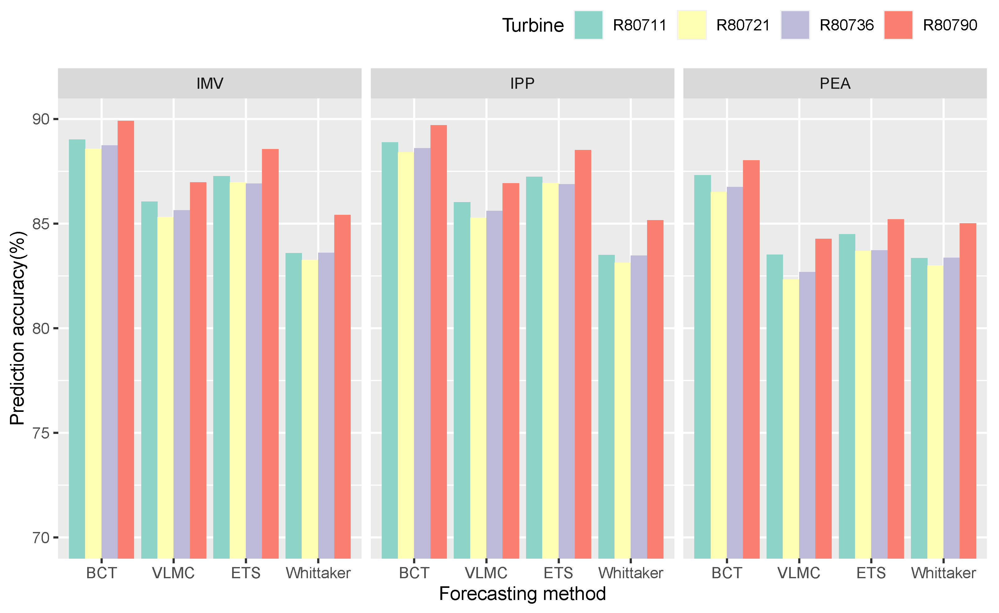
| La Haute Borne | BCT | R80711 | 89.02 | 29.89 | 88.89 | 87.32 |
| R80721 | 88.58 | 27.64 | 88.42 | 86.51 | ||
| R80736 | 88.74 | 27.96 | 88.60 | 86.75 | ||
| R80790 | 89.91 | 20.05 | 89.71 | 88.03 | ||
| VLMC | R80711 | 86.06 | 32.81 | 86.02 | 83.52 | |
| R80721 | 85.31 | 32.53 | 85.29 | 82.33 | ||
| R80736 | 85.64 | 33.65 | 85.61 | 82.68 | ||
| R80790 | 86.97 | 24.37 | 86.93 | 84.27 | ||
| ETS | R80711 | 87.27 | 39.53 | 87.24 | 84.50 | |
| R80721 | 86.98 | 36.65 | 86.95 | 83.70 | ||
| R80736 | 86.92 | 37.58 | 86.88 | 83.73 | ||
| R80790 | 88.56 | 27.37 | 88.51 | 85.21 | ||
| WS | R80711 | 83.59 | 25.08 | 83.50 | 83.36 | |
| R80721 | 83.26 | 24.49 | 83.13 | 83.00 | ||
| R80736 | 83.61 | 24.66 | 83.47 | 83.37 | ||
| R80790 | 85.41 | 20.76 | 85.17 | 85.02 | ||
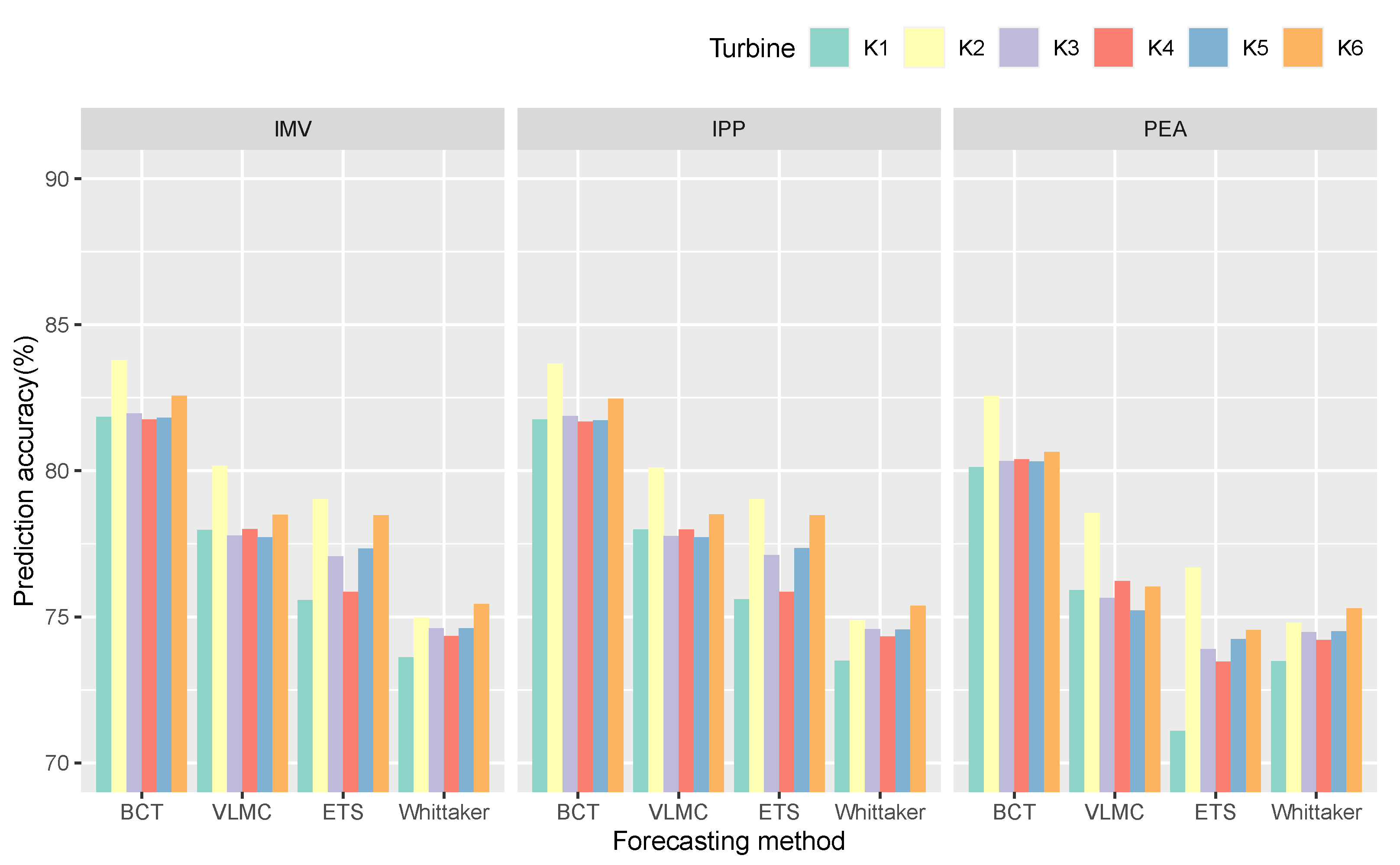
| Kelmarsh | BCT | K1 | 81.85 | 38.82 | 81.75 | 80.13 |
| K2 | 83.79 | 41.46 | 83.67 | 82.56 | ||
| K3 | 81.96 | 39.18 | 81.87 | 80.34 | ||
| K4 | 81.76 | 40.50 | 81.68 | 80.39 | ||
| K5 | 81.81 | 39.78 | 81.73 | 80.32 | ||
| K6 | 82.57 | 36.43 | 82.47 | 80.65 | ||
| VLMC | K1 | 77.98 | 40.90 | 77.99 | 75.91 | |
| K2 | 80.17 | 51.90 | 80.11 | 78.56 | ||
| K3 | 77.78 | 41.48 | 77.76 | 75.64 | ||
| K4 | 78.01 | 50.48 | 77.99 | 76.23 | ||
| K5 | 77.73 | 49.75 | 77.72 | 75.22 | ||
| K6 | 78.50 | 45.81 | 78.51 | 76.03 | ||
| ETS | K1 | 75.57 | 45.31 | 75.60 | 71.09 | |
| K2 | 79.03 | 48.35 | 79.03 | 76.69 | ||
| K3 | 77.07 | 45.75 | 77.12 | 73.90 | ||
| K4 | 75.86 | 50.99 | 75.86 | 73.46 | ||
| K5 | 77.33 | 47.44 | 77.35 | 74.23 | ||
| K6 | 78.48 | 42.76 | 78.48 | 74.55 | ||
| WS | K1 | 73.61 | 29.79 | 73.50 | 73.48 | |
| K2 | 74.98 | 30.68 | 74.89 | 74.80 | ||
| K3 | 74.61 | 30.81 | 74.58 | 74.47 | ||
| K4 | 74.34 | 30.23 | 74.32 | 74.21 | ||
| K5 | 74.61 | 30.91 | 74.57 | 74.51 | ||
| K6 | 75.44 | 29.52 | 75.38 | 75.29 | ||
References
- IPCC. Summary for Policymakers. In Climate Change 2023: Synthesis Report. Contribution of Working Groups I, II and III to the Sixth Assessment Report of the Intergovernmental Panel on Climate Change; Lee, H., Romero, J., Eds.; IPCC: Geneva, Switzerland, 2023; pp. 1–34. [Google Scholar] [CrossRef]
- IRENA. Renewable Power Generation Costs in 2022; International Renewable Energy Agency: Abu Dhabi, United Arab Emirates, 2023; Available online: https://www.irena.org/Publications/2023/Aug/Renewable-Power-Generation-Costs-in-2022 (accessed on 30 January 2024).
- IRENA. Renewable Energy Statistics 2023; International Renewable Energy Agency: Abu Dhabi, United Arab Emirates, 2023; Available online: https://www.irena.org/Publications/2023/Jul/Renewable-energy-statistics-2023 (accessed on 30 January 2024).
- Ding, Y. Data Science for Wind Energy; CRC Press: Boca Raton, FL, USA, 2019; p. 95. ISBN 978-04-2995-651-5. [Google Scholar]
- IEC 61400-12-1:2022. Available online: https://iss.rs/en/project/show/iec:proj:17046 (accessed on 29 May 2023).
- Anahua, E.; Barth, S.; Peinke, J. Markovian power curves for wind turbines. Wind. Energ. 2007, 11, 219–232. [Google Scholar] [CrossRef]
- Pedersen, T.F.; Wagner, R.; Demurtas, G. Wind Turbine Performance Measurements by Means of Dynamic Data Analysis; DTU Wind Energy: Roskilde, Denmark, 2016; ISBN 978-87-93278-28-8. [Google Scholar]
- Janssens, O.; Noppe, N.; Devriendt, C.; Van de Walle, R.; Van Hoecke, S. Data-driven multivariate power curve modeling of offshore wind turbines. Eng. Appl. Artif. Intell. 2016, 55, 331–338. [Google Scholar] [CrossRef]
- Qiao, Y.; Han, S.; Zhang, Y.; Liu, Y.; Yan, J. A multivariable wind turbine power curve modeling method considering segment control differences and short-time self-dependence. Renew. Energy 2024, 222, 119894. [Google Scholar] [CrossRef]
- Sebastiani, A.; Peña, A.; Troldborg, N. Numerical evaluation of multivariate power curves for wind turbines in wakes using nacelle lidars. Renew. Energy 2022, 202, 419–431. [Google Scholar] [CrossRef]
- Dhont, M.; Tsiporkova, E.; Boeva, V. Layered Integration Approach for Multi-view Analysis of Temporal Data. In Advanced Analytics and Learning on Temporal DataIn Advanced Analytics and Learning on Temporal Data—5th ECML PKDD Workshop AALTD 2020 Revised Selected Papers; Lemaire, V., Malinowski, S., Bagnall, A., Guyet, T., Tavenard, R., Ifrim, G., Eds.; Springer International Publishing AG: Cham, Switzerland, 2020; Volume 12588, pp. 138–154. [Google Scholar] [CrossRef]
- Dhont, M.; Tsiporkova, E.; Boeva, V. Advanced Discretisation and Visualisation Methods for Performance Profiling of Wind Turbines. Energies 2021, 14, 6216. [Google Scholar] [CrossRef]
- Astolfi, D.; Pandit, R. Multivariate Wind Turbine Power Curve Model Based on Data Clustering and Polynomial LASSO Regression. Appl. Sci. 2022, 12, 72. [Google Scholar] [CrossRef]
- Zhang, X.; Jia, J.; Zheng, L.; Yi, W.; Zhang, Z. Maximum Power Point Tracking Algorithms for Wind Power Generation System: Review, Comparison, and Analysis. Energy Sci. Eng. 2023, 11, 430–444. [Google Scholar] [CrossRef]
- Weiss, C.H. An Introduction to Discrete-Valued Time Series; John Wiley & Sons Ltd.: Hoboken, NJ, USA, 2018; ISBN 978-11-19097-01-3. [Google Scholar]
- Bühlmann, P.; Wyner, A.J. Variable length Markov chains. Ann. Stat. 1999, 27, 480–513. [Google Scholar] [CrossRef]
- Rissanen, J. A Universal Data Compression System. IEEE Trans. Inf. Theory 1983, 29, 656–664. [Google Scholar] [CrossRef]
- Kontoyiannis, I.; Mertzanis, L.; Panotopoulou, A.; Papageorgiou, I.; Skoularidou, M. Bayesian Context Trees: Modelling and Exact Inference for Discrete Time Series. J. R. Stat. Soc. B. 2022, 84, 1287–1323. [Google Scholar] [CrossRef]
- Sarkar, A.; Dunson, D.B. Bayesian Nonparametric Modeling of Higher Order Markov Chains. J. Am. Stat. Assoc. 2016, 111, 1791–1803. [Google Scholar] [CrossRef]
- Hyndman, R.; Koehler, A.B.; Ord, J.K.; Snyder, R.D. Forecasting with Exponential Smoothing: The State Space Approach; Springer Science & Business Media: Berlin, Germany, 2008. [Google Scholar] [CrossRef]
- Eilers, P.H.C. A perfect smoother. Anal. Chem. 2003, 75, 3631–3636. [Google Scholar] [CrossRef] [PubMed]
- La Haute Borne Wind Farm. Available online: https://opendata-renewables.engie.com/explore/ (accessed on 3 April 2023).
- Plumley, C. Kelmarsh Wind Farm Data. Zenodo, 2022. Available online: https://doi.org/10.5281/zenodo.5841833 (accessed on 29 May 2023).
- MacQueen, J. Some methods for classification and analysis of multivariate observations. In Proceedings of the Fifth Berkeley Symposium on Mathematical Statistics and Probability, Oakland, CA, USA, 21 June–18 July 1967; Volume 1, pp. 281–297. [Google Scholar]
- Handl, J.; Knowles, J.; Kell, D.B. Computational Cluster Validation in Post-Genomic Data Analysis. Bioinformatics 2005, 21, 3201–3212. [Google Scholar] [CrossRef] [PubMed]
- Rousseeuw, P.J. Silhouettes: A graphical aid to the interpretation and validation of cluster analysis. J. Comput. Appl. Math. 1987, 20, 53–65. [Google Scholar] [CrossRef]
- Caliński, T.; Harabasz, J. A dendrite method for cluster analysis. Commun. Stat.-Theory Methods 1974, 3, 1–27. [Google Scholar] [CrossRef]
- Davies, D.L.; Bouldin, D.W. A Cluster Separation Measure. IEEE Trans. Pattern Anal. Mach. Intell. 1979, PAMI-1, 224–227. [Google Scholar] [CrossRef]
- Tjalkens, T.J.; Willems, F.M.J.; Shtarkov, Y.M. Multi-alphabet universal coding using a binary decomposition context tree weighting algorithm. In Proceedings of the 15th Symposium on Information Theory in the Benelux, Louvain-la-Neuve, Belgium, 30–31 January 1994; pp. 259–265. [Google Scholar]
- Willems, F.; Shtarkov, Y.; Tjalkens, T. The context-tree weighting method: Basic properties. IEEE Trans. Inf. Theory 1995, 41, 653–664. [Google Scholar] [CrossRef]
- Mächler, M.; Bühlmann, P. Variable length Markov chains: Methodology, computing, and software. J. Comput. Graph. Stat. 2004, 13, 435–455. [Google Scholar] [CrossRef]
- Whittaker, E.T. On a New Method of Graduation. Proceedings of the Edinburgh Mathematical Society. Proc. Edinburgh Math. Soc. 1923, 41, 63–75. [Google Scholar] [CrossRef]
- Shumway, R.H.; Stoffer, D.S. Time Series Analysis and Its Applications: With R Examples, 4th ed.; Springer: Cham, Switzerland, 2017; ISBN 978-3-319-52452-8. [Google Scholar]
- Evchenko, M.; Vanschoren, J.; Hoos, H.H.; Schoenauer, M.; Sebag, M. Frugal Machine Learning. arXiv 2021, arXiv:2111.03731. [Google Scholar]
- Weissman, T.; Ordentlich, E.; Seroussi, G.; Verdú, S.; Weinberger, M.J. Universal discrete denoising: Known channel. IEEE Trans. Inf. Theory 2005, 51, 5–28. [Google Scholar] [CrossRef]
- Zheng, X.; Dumitrescu, B.; Liu, J.; Giurcăneanu, C.D. Multivariate Time Series Imputation: An Approach Based on Dictionary Learning. Entropy 2022, 24, 1057. [Google Scholar] [CrossRef] [PubMed]


| Description | R80711 | R80721 | R80736 | R80790 |
|---|---|---|---|---|
| Time-series length | 210,384 | |||
| Missing values | ||||
| Total number | 39,840 | 47,107 | 45,491 | 71,147 |
| Percentage | 18.9% | 22.4% | 21.6% | 34.0% |
| Sequence length | ||||
| Longest | 1341 | 800 | 293 | 36,358 |
| Second Longest | 397 | 724 | 277 | 499 |
| Shortest | 1 | 1 | 1 | 1 |
| Mean | 12.38 | 12.90 | 12.62 | 24.58 |
| Median | 3 | 3 | 3 | 3 |
| Description | K1 | K2 | K3 | K4 | K5 | K6 |
|---|---|---|---|---|---|---|
| Time-series length | 236,448 | |||||
| Missing Values | ||||||
| Total number | 32,537 | 26,472 | 31,656 | 28,140 | 29,738 | 38,954 |
| Percentage | 13.8% | 11.2% | 13.4% | 12.0% | 12.6% | 16.5% |
| Sequence Length | ||||||
| Longest | 2344 | 2109 | 2109 | 2109 | 2109 | 4064 |
| Second Longest | 2109 | 1538 | 1675 | 1539 | 1537 | 2110 |
| Shortest | 1 | 1 | 1 | 1 | 1 | 1 |
| Mean | 6.79 | 8.86 | 8.34 | 8.71 | 8.20 | 9.02 |
| Median | 1 | 2 | 2 | 2 | 2 | 2 |
| Wind Farm | Turbine | IMV | IPP | PEA | |
|---|---|---|---|---|---|
| Accuracy (%) | Time (min) | Accuracy (%) | Accuracy (%) | ||
| La Haute Borne | R80711 | 89.02 | 29.89 | 88.99 | 87.32 |
| R80721 | 88.58 | 27.64 | 88.42 | 86.51 | |
| R80736 | 88.74 | 27.96 | 88.60 | 86.75 | |
| R80790 | 89.91 | 20.05 | 89.71 | 88.03 | |
| Kelmarsh | K1 | 81.85 | 38.82 | 81.75 | 80.13 |
| K2 | 83.79 | 41.46 | 83.67 | 82.56 | |
| K3 | 81.96 | 39.18 | 81.87 | 80.34 | |
| K4 | 81.76 | 40.50 | 81.68 | 80.39 | |
| K5 | 81.81 | 39.78 | 81.73 | 80.32 | |
| K6 | 82.57 | 36.43 | 82.47 | 80.65 | |
| Wind Farm | Forecasting Method | Turbine | IMV | PEA | |
|---|---|---|---|---|---|
| Accuracy (%) | Time | Accuracy (%) | |||
| La Haute Borne | BCT | R80711 | 91.67 | 2.42 | 90.14 |
| R80721 | 91.50 | 2.13 | 89.43 | ||
| R80736 | 92.01 | 2.06 | 89.97 | ||
| R80790 | 92.94 | 1.86 | 90.64 | ||
| CTF | R80711 | 91.35 | 540.44 | 88.39 | |
| R80721 | 91.13 | 484.05 | 88.42 | ||
| R80736 | 91.60 | 495.09 | 89.18 | ||
| R80790 | 92.17 | 481.13 | 89.55 | ||
| Kelmarsh | BCT | K1 | 83.32 | 3.39 | 81.49 |
| K2 | 84.48 | 3.51 | 83.47 | ||
| K3 | 85.60 | 3.18 | 83.83 | ||
| K4 | 84.27 | 3.24 | 82.77 | ||
| K5 | 83.22 | 3.12 | 80.96 | ||
| K6 | 83.77 | 3.40 | 81.47 | ||
| CTF | K1 | 81.69 | 611.66 | 78.07 | |
| K2 | 82.82 | 615.92 | 80.36 | ||
| K3 | 83.86 | 636.26 | 81.57 | ||
| K4 | 81.85 | 631.48 | 79.55 | ||
| K5 | 81.42 | 592.16 | 78.12 | ||
| K6 | 82.23 | 635.40 | 78.67 | ||
Disclaimer/Publisher’s Note: The statements, opinions and data contained in all publications are solely those of the individual author(s) and contributor(s) and not of MDPI and/or the editor(s). MDPI and/or the editor(s) disclaim responsibility for any injury to people or property resulting from any ideas, methods, instructions or products referred to in the content. |
© 2024 by the authors. Licensee MDPI, Basel, Switzerland. This article is an open access article distributed under the terms and conditions of the Creative Commons Attribution (CC BY) license (https://creativecommons.org/licenses/by/4.0/).
Share and Cite
Yun, H.; Giurcăneanu, C.D.; Dobbie, G. Several Approaches for the Prediction of the Operating Modes of a Wind Turbine. Electronics 2024, 13, 1504. https://doi.org/10.3390/electronics13081504
Yun H, Giurcăneanu CD, Dobbie G. Several Approaches for the Prediction of the Operating Modes of a Wind Turbine. Electronics. 2024; 13(8):1504. https://doi.org/10.3390/electronics13081504
Chicago/Turabian StyleYun, Hannah, Ciprian Doru Giurcăneanu, and Gillian Dobbie. 2024. "Several Approaches for the Prediction of the Operating Modes of a Wind Turbine" Electronics 13, no. 8: 1504. https://doi.org/10.3390/electronics13081504
APA StyleYun, H., Giurcăneanu, C. D., & Dobbie, G. (2024). Several Approaches for the Prediction of the Operating Modes of a Wind Turbine. Electronics, 13(8), 1504. https://doi.org/10.3390/electronics13081504