Article

Evaluation of Entropy Analysis as a Fault-Related Feature for Detecting Faults in Induction Motors and Their Kinematic Chain

by
Arturo Y. Jaen-Cuellar
1,
Juan J. Saucedo-Dorantes
1,
David A. Elvira-Ortiz
1 and
Rene de J. Romero-Troncoso
2,*
1
Academic Center of Advanced and Sustainable Technology (CATAS), Tequisquiapan Campus, Autonomous University of Queretaro, Carretera No. 120, San Juan del Río-Xilitla, Km 19+500, Tequisquiapan 76750, Queretaro, Mexico
2
HSPdigital CA-Mecatronica Engineering Faculty, Autonomous University of Queretaro, San Juan del Rio 76806, Queretaro, Mexico
*
Author to whom correspondence should be addressed.
Electronics 2024, 13(8), 1524; https://doi.org/10.3390/electronics13081524
Submission received: 12 March 2024 / Revised: 11 April 2024 / Accepted: 15 April 2024 / Published: 17 April 2024

Abstract

:
The induction motors found in industrial and commercial applications are responsible for most of the energy consumption in the world. These machines are widely used because of their advantages like high efficiency, robustness, and practicality; nevertheless, the occurrence of unexpected faults may affect their proper operation leading to unnecessary breakdowns with economic repercussions. For that reason, the development of methodologies that ensure their proper operation is very important, and in this sense, this paper presents an evaluation of signal entropy as an alternative fault-related feature for detecting faults in induction motors and their kinematic chain. The novelty and contribution lie in calculating a set of entropy-related features from vibration and stator current signals measured from an induction motor operating under different fault conditions. The aim of this work is to identify changes and trends in entropy-related features produced by faulty conditions such as broken rotor bars, damage in bearings, misalignment, unbalance, as well as different severities of uniform wear in gearboxes. The estimated entropy-related features are compared to other classical features in order to determine the sensitivity and potentiality of entropy in providing valuable information that could be useful in future work for developing a complete methodology for identifying and classifying faults. The performed analysis is applied to real experimental data acquired from a laboratory test bench and the obtained results depict that entropy-related features can provide significant information related to particular faults in induction motors and their kinematic chain.

1. Introduction

The industry has been constantly subjected to changes due to the emerging technology up to its relatively new version known as Industry 4.0, and despite the technological improvements with views towards efficient energy consumption, it still strongly depends on the use of electrical and mechanical elements such as gearboxes (GBs), induction motors (IMs), and their associated kinematic chains to propel most of their processes [1,2]. Some of the most common applications of GBs and IMs are [3,4,5] conveyors, pumps, cranes, fans, lifts, shredders, blowers, benders, and mixers, among others. The main characteristics of GB and IM are their general robustness, variety of prices and models, power–speed adjustable relationship, reliability, high-efficiency, easy maintenance, wide applicability, and hard environmental resistance [6,7]. Certainly, the use of IMs allows for the maximization of the productivity and reliability of the processes, but, in consequence, it must be kept in optimal conditions to ensure its continuous working without undesirable and unexpected production breakdowns [8]. In fact, IMs remain the most used electromechanical equipment and they may be found in approximately 80% of all industrial applications [9,10]. Accordingly, its wide use leads to the production of between 40% and 60% of the world’s energy consumption according to the International Energy Agency and other research works [4,5,11,12]. For that reason, it is mandatory to ensure the correct operation of the IMs and their associated kinematic chain through adequately scheduled preventive maintenance; otherwise, it could result in severe economic losses, equipment damage, or human injuries [10]. In summary, the analysis and study of these machines are currently active since there are some challenges that have not been previously addressed in reported works, i.e., the detection and identification of faults regardless of the operating condition. For that reason, the development of new approaches using novel and non-conventional features is still required, to complement, or not, the existing methodologies for increasing the performance in the diagnostic.
Regarding the reported methodologies in the literature for detecting and classifying faults on IMs, there are two general strategies that can be identified: (1) classical methodologies and (2) Data-Driven-based Approaches (DDA). Most of the classical methodologies apply conventional techniques over measured signals in the time, frequency, and time–frequency domains to visualize abnormal behaviors related to the occurrence of faults [13,14]; the most used techniques are the Fast Fourier Transform (FFT), the Discrete Wavelet Transform (DWT), and the Multiple Signal Classification (MUSIC), among others. Although these techniques have demonstrated their effectiveness, some challenges and limitations have not been completely addressed. Hence, limitations such as the strong dependency on the spectral content and the overlapping of some fault-related frequencies can increase the degree of difficulty in differentiating between different faulty conditions. Accordingly, some challenges that have to be faced are the resolution requirements of the spectral-based methods, the adequate selection of a mother function in DWT-based methods, the selection of adequate decomposition levels in empirical mode decomposition, or the expert knowledge required in advance due to the technique complexity, to mention a few [15]. On the other hand, the data-driven-based approaches are strategies for decision making based on the analysis and interpretation of data, and they take advantage of their powerful capabilities for processing high amounts of data and grouping them as clusters, such as the Principal Component Analysis (PCA), the Linear Discriminant Analysis (LDA), k-Nearest Neighbors (kNN), and Dictionary Learning (DicL), among others [4,16,17]. Nevertheless, the common drawbacks of these techniques comprise the need to use historical or high volumes of collected data, where a low volume of data could yield misleading labeling, the application of the techniques being limited to the data used for training, the propensity to overfitting, data can be biased, in many cases there exists a requirement of additional data pre-processing prior to apply the clustering mechanisms, and so on [18]. Some schemes under the DDA are the Shallow Machine Learning (SML) approaches, which combine, in general, the feature extraction, such as statistical features, frequency features, etc., with some classifiers, like Fuzzy Logic (FL), Artificial Neural Networks (ANN), Support Vectors Machine (SVM), and so on, for categorizing the faults [19,20]. The general weaknesses of these techniques are the processing of a high number of features, the estimation of redundant or correlated information in the feature calculation stage, the technique overfitting, the adequate selection of the mechanisms for feature extraction, the classifier configuration, and the optimal values of the techniques hyperparameters, to mention a few [21]. Additionally, a subset of the SML approaches is the Deep Learning (DL) techniques, which are schemes that take advantage of new reinforced structures based on neural networks such as Sparse Auto-encoder (SAE), Convolutional Neural Networks (CNN), Self-organizing Maps (SOM), Generative Adversarial Networks (GAN), Expandable Continuous Learning (ECL), and Transfer Learning (TL), among others [22,23,24,25,26]. These structures are capable of learning features, patterns, profiles, and clues with the aim of directly classifying the faults from the signals in the time, frequency, and time–frequency domains, or from features computed from any of these domains. Furthermore, recent research has led to some improvements; for example, GAN, ECL, and TL have integrated intelligent fault diagnosis by adding data augmentation properties, extending the learning capability through elastic expansion mechanisms that progressively introduce new network branches, or combining the transfer learning to the DL techniques [24,25,26]. These intelligent approaches overcome limitations of DL such as the incapability of processing a low volume of data samples, fusing diverse information, augmenting the representation learning capability, anticipating the influence of variability in working conditions, and speeding up the training processes. However, the main disadvantages of the DL techniques are the expertise and knowledge required to define the structure of the network, the selection of their optimal hyperparameters to guarantee the best performance for the faults diagnostic, misleading diagnosis for multiple or combined faults with similar response behavior, non-linearities, non-stationary behavior, data quantity/quality/complexity, and noise addition [27]. In this sense, recent works have also directed towards the use of non-conventional feature extraction, for example, metrics related to the behavior of the signal energy, such as entropy.
Several works have been developed considering non-conventional indicators in applications related to the detection of abnormal conditions in industrial equipment, such as the entropy calculation [28,29,30,31]. For example, in [32], twelve entropy-based features were extracted from vibration signals in time, frequency, and time–frequency domains for detecting problems in bearings, and a Z-score was used as a threshold of the features for showing the fault. Under the same framework, a theoretical review was developed in [31], where the entropy measurements related to the statistical mechanics, the information theory, and the dynamical systems theory were analyzed to give some insights about its potential for detecting bearing faults. The research in [33] presents a methodology for diagnosing faults in bearings by decomposing the vibration signal through the Wavelet Packet Transform (WPT) and, at the same time, it computes the Teager energy entropy ratio of the resonant frequency sub-band. Likewise, in other work, an approach for monitoring the conditions of rolling bearings in wind turbines is developed [34]. Firstly, the vibration signal is decomposed through the Variational Mode Decomposition (VMD). Next, the statistical features are extracted, and a permutation entropy analysis is performed to analyze the time series complexity, then feature selection is carried out and, finally, a multi-class-SVM performs the classification task. In another example, six entropy-based features were extracted from vibration signals to automatically diagnose the bevel gear wear [35]. In that work, an analytic wavelet transform is applied to decompose the signal into sub-bands, and then the entropy features are extracted and fed to a Least-Squares Support Vector Machine (LS-SVM) classifier. Additionally, the Kruskal–Wallis test is carried out to generate statistically meaningful results. The work reported in [30] makes use of several entropy-based methods for fault classification in bearings, and they are compared to provide assessments and recommendations for future developments in new classification methodologies. On the other hand, the research described in [36] proposes an intelligent fault diagnosis through the Hierarchical Diversity Entropy (HDE) as a feature extraction tool and the Random Forest (RF) classifier for detecting early bearing faults from signals with high noise levels and weak fault symptoms. In another case, a methodology that proposes to combine a Multiscale Weighted Permutation Entropy (MWPE) with a Twin Extreme Learning Machine (TELM) for extracting enhanced features with non-stationary and non-linear characteristics is developed in [37]. In another field, the work in [38] presents a hybrid methodology between VMD, permutation entropy, and k-means clustering for selecting a low-resistance grounding fault line. Here, the VMD serves to reduce the influence of harmonic content and noise to facilitate feature extraction. From the previously analyzed works, it is important to mention that entropy features have some pros and cons that are worth mentioning; for example, as cons, the direct feature extraction from time domain signals could be ineffective depending on the noise level, and also the extraction of entropy features could be enhanced through a multiscale or multiscale weighted approach [37,38]. In contrast, the pros are that several novel methods to enhance classical fault detection can be developed using entropy features; for example, they can address systems with non-linearities and non-stationary characteristics, even with non-linear time series complexity, but also they provide consistency, strong robustness, and high calculation efficiency [28,29,31,36,37,38]. Regarding the field of rotative machinery, most of the reported works have focused their efforts on studying the faults in bearing elements due to the frequency relation to the entropy calculation, but other type of faults related to the kinematic chain of the motor could be addressed, such as coupling misalignment, system unbalance, or gears wear in gearboxes. In summary, any non-conventional features, like those based in the entropy that helps to provide clues of the different conditions of a system, are still considered a field of interest and their validation through correlation tests could be a relevant aspect for the detection of faults in IMs and the associated kinematic chain.
Therefore, the contribution of this work lies in evaluating the use of entropy features to determine its discriminant properties for condition monitoring of faults that may unexpectedly occur in gearboxes, induction motors, and their related kinematic chain. To perform the entropy signal analysis, this work proposes the calculation of six entropy parameters such as spectral, permutation, sample, approximated, fuzzy, and Rényi entropy; these features are estimated from different available physical magnitudes, like vibration signals and stator current signatures, which are acquired during different experimental tests. Four different severities of uniform wear are tested in the gearbox and in the induction motor conditions like bearing defect, broken rotor bar, unbalance, and misalignment are evaluated, and each of the aforementioned conditions is iteratively tested in the gearbox and the induction motor under different operating conditions. The entropy features are extracted, and further processing is performed to assess the operating condition of the IM and the related kinematic chain. In a sense of a complement tool, the entropy features are analyzed to demonstrate which of them provide meaningful and discriminant information that could improve the efficiency of classical approaches; meaning that when entropy indicators are used, they allow a more efficient discrimination of failure conditions. Additionally, the validation of the features is essential, and verification mechanisms are also important; for this reason, the Kruskal–Wallis test and the Fisher discriminant score could in a reliable way enhance the proposed analysis. The obtained results show that entropy features have advantages for the detection of faults, compared to other methods, which can be used to improve the detection efficiency.

2. Theoretical Background
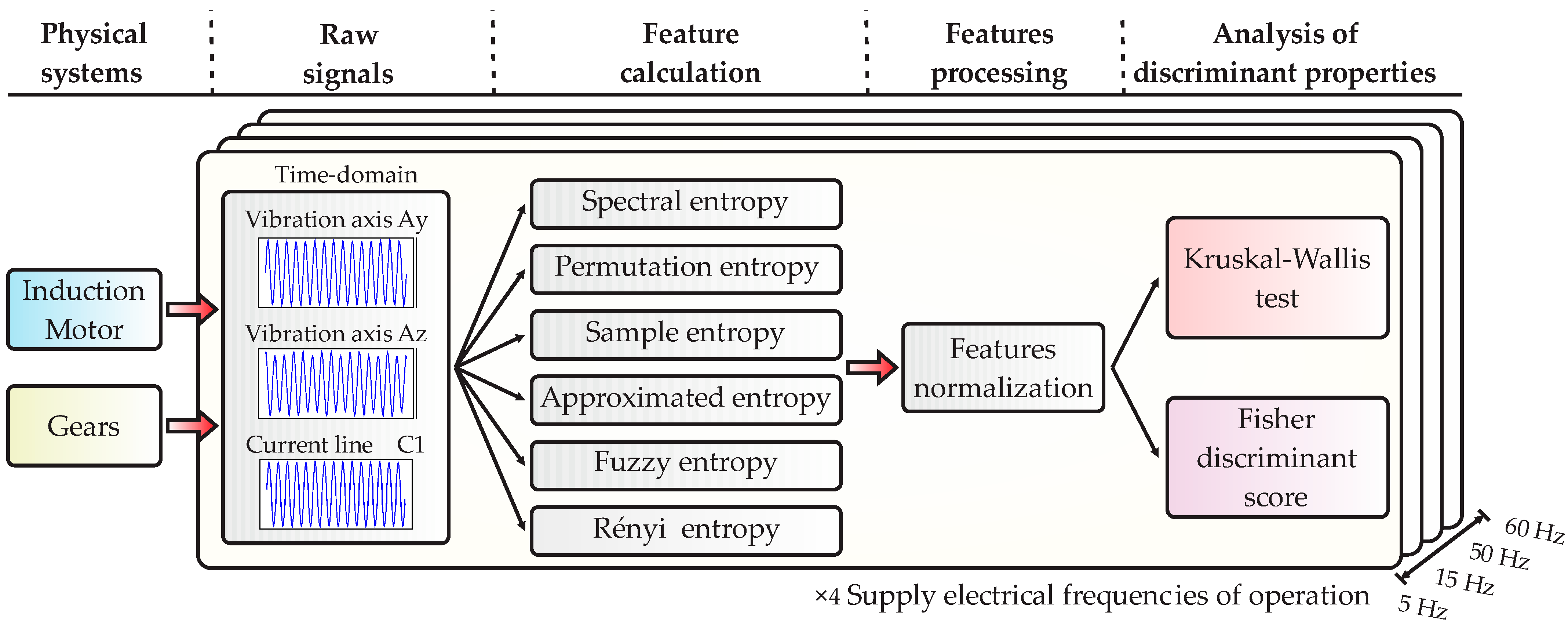
Entropy is a physical magnitude that has been widely studied in physics and thermodynamics. This magnitude is commonly associated with the degree of disorder in a system; however, a most formal definition derives from the second law of thermodynamics that establishes that every system evolves to its most probable configuration, as this is the one with the most microstates, and it coincides with the one with the greatest entropy. In this sense, entropy can be explained as a measure of the probability that a system reaches a specific final state based on the number of different configurations that lead to such a final state [35]. In other words, the more different configurations that lead to the same final state, the higher the probability of reaching that state and the greater the entropy is. This notion of entropy has been employed in the field of data analytics and signal processing to determine the possible causes of a signal obtaining a specific trend, allowing us to explain how two different phenomena are related to each other. The most used expression for quantifying the entropy of a signal or dataset was introduced by Claude E. Shannon in 1948 [31,39], and it is shown in Equation (1).
H X = i = 1 n p x i log p x i
where H ( X ) is the Shannon entropy of the signal X ; x i is the i -th element of the signal X ; and p x i is the probability that the value x i appears in the signal.
Although the Shannon entropy is good for detecting irregularities in a signal, some variants have been developed to increase the accuracy and performance of this feature. For instance, when it is necessary to estimate the complexity of the data, the spectral entropy ( S p e c E n ) is a better feature. The spectral entropy needs to compute the spectrum of the signal X using the Fourier transform and calculate the power of each frequency component ( p f ); thus, the spectral entropy is finally obtained using Equation (2).
S p e c E n X = f p f log 1 p f
Another variant of the Shannon entropy that works better in the quantification of uncertainty and randomness in time series is the Rényi entropy ( R e E n ). This is a generalization of the Shannon entropy that can be computed using Equation (3).
R e E n X = α 1 α i = 1 n log 2 p x i α
where p ( x i ) is the probability of the time series X = x 1 ,   x 2 ,   ,   x n , and α   1 represents the order of the feature. Regarding the parameter α , it is common to use values higher than 2 to obtain smoother results. Moreover, if α = 1 , then the Rényi entropy becomes the Shannon entropy.
In some applications, it is also required to know the irregularity and unpredictability of the time series, and the approximate entropy ( A p E n ) is the preferred tool for such a task. This feature can assess the probability that a new pattern appears in the signal behavior, and it can be expressed as shown in Equation (4).
A p E n X = ϕ m r ϕ m + 1 r
where ϕ m r and ϕ m + 1 r are the mean values of the logarithm pattern and they are calculated according to Equation (5).
ϕ m r = 1 N m + 1 i = 1 N m + 1 ln 1 N m + 1 n u m d x i , x j < r
where m is the length of the pattern, r = 0.2 S D (with S D as the standard deviation of the signal) is the tolerance of the signal, N is the length of the signal, and n u m d x i , x j < r is the distance between the terms x i and x j . To achieve better results in the literature, it is recommended to use a value of m = 2 for the pattern length [29]. The A p E n presents some immunity against interference and noise, but it is highly dependent on the signal length, and small signals usually deliver unexpected results. Additionally, the estimation regarding the complexity of the signal is not very accurate. Therefore, to overcome the issues related to the A p E n , it was developed the sample entropy ( S a m p E n ) that can be calculated using Equation (6).
S a m p E n = ln B m + 1 r B m r
where B m r and B m + 1 r are the mean values of the pattern count, and they can be obtained through Equation (7).
B m r = 1 N m + 1 i = 1 N m + 1 1 N m n u m d x i ,   x j < r
where r is the tolerance of the signal, m is the embedding dimension, N is the signal length, and n u m d x i ,   x j < r is the distance between x i and x j with i = 1 ,   2 ,   ,   N m + 1 , and i j .
Also, the fuzzy entropy (FuzEn) is an important feature that allows us to determine the similarity between two signals [28]. In this sense, the similarity can be expressed by Equation (8).
S i j m = e ln 2 d i j m r n
where m is the embedding dimension, d i j m is the distance between the samples x i m and x j m , and r is the similarity tolerance. Also, the operator φ m ( N , r ) must be defined as in Equation (9).
φ m N , r = 1 N m i = 1 N m 1 N m + 1 j = 1 ,   j i N m S i j m
With N being the length of the signal, therefore, the F u z E n can be calculated as Equation (10) depicts.
F u z E n m , r , N = ln φ m N , r ln φ m + 1 ( N , r )
On its part, the permutation entropy ( P e r m E n ) also allows us to estimate the complexity of a signal, with the difference that it uses a phase space reconstruction to compute the complexity [30]. This is a particularly good approach for dealing with signals that introduce non-linearities. The permutation entropy is calculated using Equation (11).
P e r m E n = p π log 2 p ( π )
where p ( π ) is the relative frequency for each permutation.
Together, all these entropy variations can provide information regarding the anomalies and disturbances in a signal and how these variations are related to a specific operating condition in a system such as an induction motor.

3. Methodology

As mentioned above, it is still a field of interest in the development of new diagnosis methodologies capable of distinguishing between different fault conditions that a machine could present. In this sense, Figure 1 presents the general flow chart of the approach proposed in this work, which is focused on an analysis of six different entropy features that are estimated from raw signals coming from data banks of an induction motor with fault conditions, with the main purpose of finding the discriminant properties for distinguishing the conditions of the motor (faults). Thus, the proposed approach is developed through five main stages: (i) physical systems, (ii) raw signals, (iii) feature calculation, (iv) feature processing, and (v) analysis of discriminant properties.

3.1. Physical Systems

The entropy signal analysis developed in this work is considered to be a physical system that is an experimental test bench based on a kinematic chain composed of a three-phase IM, a 4:1 ratio gearbox (GB), and a DC generator acting as mechanical load (ML). In this kinematic chain, the three-phase motor speed is controlled by a variable frequency drive (VFD), and the experimental trials were run at four different supply electrical frequencies of operation: 5 Hz, 15 Hz, 50 Hz, and 60 Hz. Next, in the kinematic chain, the motor is mechanically coupled to the gearbox, which, in turn, is coupled to the DC generator. It must be highlighted that the DC generator represents a low mechanical load, entailing around 20% of the nominal load. The configuration of the low-level load is important because it can produce a downloading effect, which causes misleading fault detection, which is a challenge for the diagnostic in classic methodologies [40,41]. Thus, the entropy analysis is explored as an alternative in fault analysis under unfavorable conditions of low load. On the other hand, the gearbox has a gear with uniform wear in all teeth, where four conditions are considered: wear of 0% (healthy gear and no wear in the teeth), wear of 25%, wear of 50%, and wear of 75%. Also, five different conditions are generated in the induction machine: healthy condition (motor without any fault), motor with bearing defect, a broken rotor bar, system unbalance, and coupling misalignment. It is important to mention that the corresponding experimental trials of every fault condition were individually carried out. The specific characteristics of the kinematic chain are explained in detail in the Section 4.

3.2. Raw Signals

The proposed analysis considers the processing of real signals that are acquired from the experimental test bench described in the previous subsection. The experimentation is carried out individually for each system condition; as a result, the corresponding measurements consider a specific fault condition stored in a data bank for further offline processing. Now, in the kinematic chain, two sensors are considered to carry out the signal measurements, that is, a triaxial vibration sensor and a current sensor based on the Hall effect. Yet, although vibrations in the kinematic chain are measured in the x , y , and z directions (axial, radial, and tangential axes), only the vibrations measured in the perpendicular plane (vibrations in the y-axis and the z-axis) of the kinematic chain rotating axis are considered in this work; such consideration is because it has been proven that this plane may experience an increase in vibrations when unexpected fault conditions appear in rotating machines [42,43]. On the other hand, only one stator current is considered to be analyzed because all the studied conditions are affected in a similar way to all the phases, hence, the stator current signature measured in the first line is taken into account. In the proposed analysis, the raw signals of the data bank are directly processed on its time-domain representation without the need for a space transform technique; the idea is to find out the usability of new features. The specific details about the sensor characteristics used in this work and the sampling frequencies considered for the data acquisition system are detailed in the Section 4.

3.3. Feature Calculation

Once the signals are measured and stored, the next step is to calculate a set of features inherent in the signals. In this case, six different features based on the entropy metric are addressed as counterparts of the classic methodologies that typically use statistical features. Thus, as observed in Figure 1, the entropy features obtained using expressions (1) to (11) are the following: SpecEn, PermEn, SampEn, ApEn, FuzEn, and ReEn. The feature calculation is carried out by segmenting each signal in equal parts of one second and then the proposed entropy features are estimated from each segmented part. The main advantages of using entropy features rely on the fact that they describe energy behavior properties of a measured signal, instead of pure data distribution as is commonly performed by classical statistical features. Moreover, entropy features also allow us to address systems with non-linearities and non-stationary characteristics, even with non-linear time series complexity, but they also provide consistency, strong robustness, and high calculation efficiency, as stated in the Introduction.

3.4. Feature Processing

The feature processing considered for the entropy features calculated from the raw signals is the data normalization. The normalization that is considered is based on the well-known approach that leads to the transformation of a signal to zero mean and unit variance, and the main purpose of normalizing the features is due to the need to visualize the capabilities of entropy features in discriminating any condition in the data, like patterns, profiles, and tendencies, among others. Additionally, it is important to consider the conventional advantages of data normalization such as minimizing and correcting duplicated data, avoiding data anomalies, optimizing the storage space, avoiding the creation of undesired relationships and dependencies between data, reducing the time and complexity in data revision, facilitating the data access and interpretation, and preventing the undesired data erasing.

3.5. Analysis of Discriminant Properties

In the final stage of this proposal, the analysis of discriminant properties is carried out. Such analysis is performed with the aim of determining the most significant fault-related properties that are inherent to the calculation of entropy features. In this regard, the discriminant properties of the entropy features are then analyzed through the Kruskal–Wallis (KW) test and by calculating their Fisher discriminant score (FDS), which are a non-parametric and parametric technique, respectively, which can be used to identify useless sample features [44,45]. Thereby, the normalized entropy features are first analyzed using the non-parametric KW test, and this test leads to the determination of whether a group of data comes from the same population, since the probability distribution is not assumed. Certainly, under a null hypothesis, the implementation of the KW test identifies whether these data come from the same distribution and in condition monitoring strategies allows us to analyze if there are statistically relevant differences between two or more categories. Hence, for C classes with n samples (per class), the test is carried out as follows [35,46]:
  • Step I: all samples ( N ) for all C classes are sorted and then a rank is assigned in ascending order by ignoring the class to which the samples belong;
  • Step II: find the sum of all R i ranks for each individual class with n i samples;
  • Step III: compute the KW statistic ( S K W ) by applying Equation (12);
  • Step IV: the significance of the resulting S K W values for all C classes are assessed through the Chi-square test ( χ 2 ); thus, the S K W values are statistically significant if S K W is equal or larger than χ 2 .
Once the KW test is performed, the p-value can be also estimated as a quantitative metric to determine if any of the differences between the medians are statistically significant; consequently, it has been determined that higher p-values are associated with statistically significant differences.
S K W = 12 N N + 1 i = 1 C R i 2 n i 3 N 1
On the other hand, the FDS is a statistical technique carried out to determine the separability between individuals (samples) that belong to different populations (classes); FDS is used in condition monitoring strategies to analyze and choose features that provide significant discriminant information [47]. Ideally, the FDS is theoretically applied to two-class problems but it has been generalized to multi-class problems; thereby, for C classes with n samples per class, the analysis through FDS considers the computation of the between-class ( S b ¯ ) and within-class ( S w ¯ ) scatter matrices following Equations (13) and (14) [48], where μ f i and μ are the mean of the k th class and the overall mean of all samples for all classes, respectively. On the other hand, x f i k represents each ith sample of the k th class. Accordingly, the estimation of S b ¯ and S w ¯ is aiming to quantify the separability between classes and to measure the compactness of data points in the same class, respectively. Hence, the FDS is achieved as a ratio ( F D S r ) between S b ¯ and S w ¯ , which measures the linear separation between two different classes, as specified in (15) [49,50]. Therefore, values of F S r higher than 1 are related to features that provide relevant discriminant information to separate the classes under analysis, whereas values of F S r smaller than 1 can lead to overlapping problems when two classes are intended to be separated.
S b ¯ = k = 1 C n k μ f i μ μ f i μ T
S w ¯ = k = 1 C i = 1 n k x f i k μ f i x f i k μ f i T
F S r = S b ¯ S w ¯
Finally, as it is observed in the block diagram of Figure 1, the proposed approach is repeated for each one of the operating frequencies that represent the supply electrical frequency of operation of the kinematic chain (5 Hz, 15 Hz, 50 Hz, and 60 Hz). Recently, the proposal of new methodologies applied to the diagnosis of faults may deal with different data distributions that are usually generated by different operating conditions like loads and speeds.

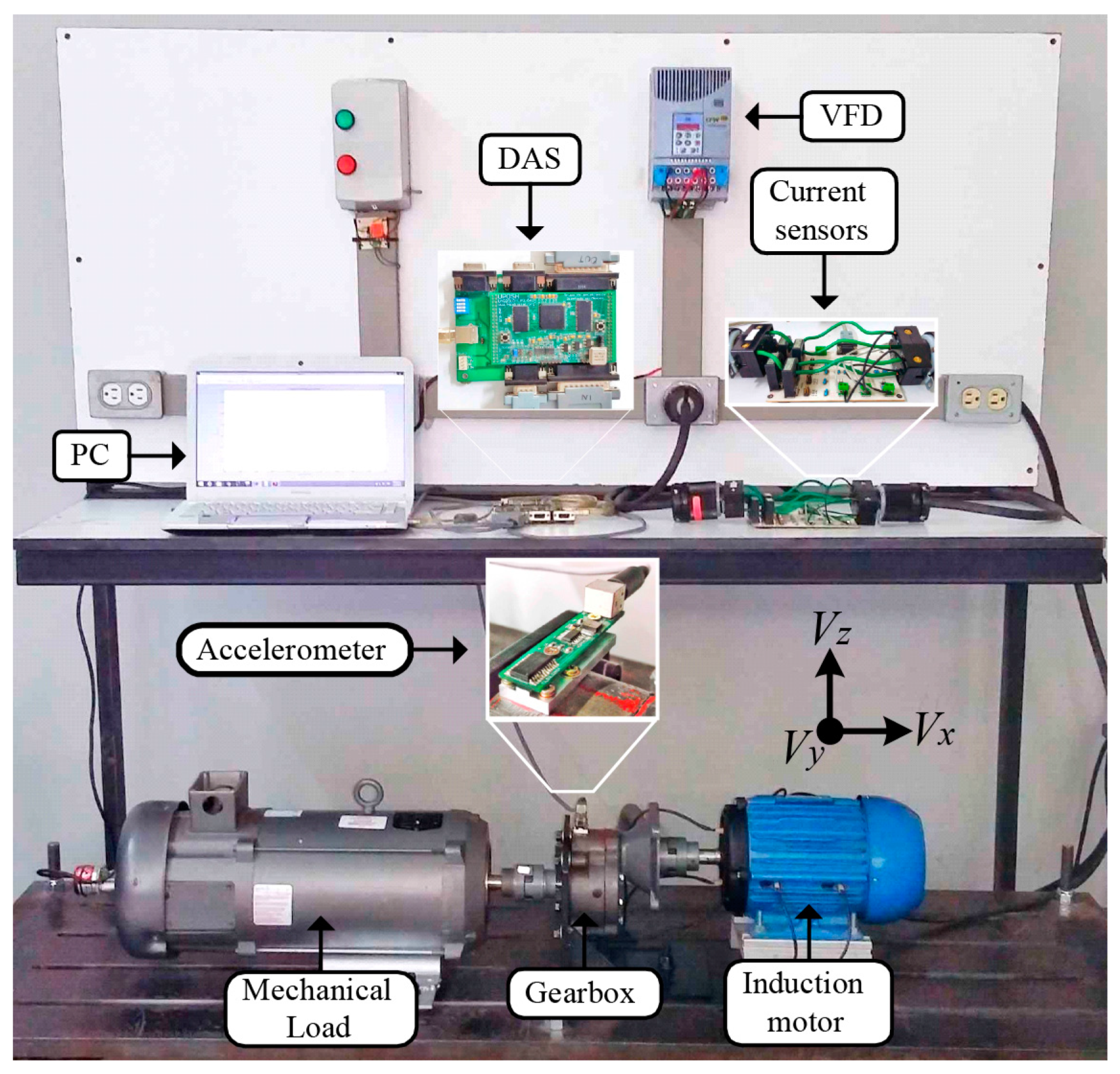
4. Experimental Setup

The analysis of signal entropy performed in this work is applied to a real dataset that is acquired from an experimental laboratory test bench, which is composed of three main elements: an IM, a GB, and a ML. The test bench is shown in Figure 2, the IM is a 2.49 kW, 220 V-three-phase motor with one pair of poles (model WEG 00236ET3E145T-W22), and it is mechanically linked to a 4:1 ratio GB (BALDOR GCF4X01AA) through a rigid coupling; the GB is, in turn, coupled to a DC generator (BALDOR CDP3604), which is used as the ML. Also, a VFD (model WEG-CFW08) is used to feed and control the rotating speed of the IM output shaft.
The dataset comprised vibration signals and stator current signatures; in this regard, the vibrations of the whole kinematic chain are acquired using a triaxial accelerometer LIS3L02AS4 that is located on the top of the GB; meanwhile, the stator currents are measured through a set of three Hall-effect sensors from Tamura Corporation (model L08P050D15) that are placed in the power supply lines between the VDF and the IM. All signals are acquired by a self-designed Data Acquisition System (DAS), which is based on Field Programmable Gate Array (FPGA) technology, the proprietary DAS has a 12-bit analog-to-digital serial-output converter (model ADS 7841) to read the available measurements. Thus, the vibration signals and stator currents are acquired with sampling frequencies equal to 3 k samples/s and 4 k samples/s, respectively.
Regarding the evaluated conditions, four conditions are tested in the GB; meanwhile, five conditions are tested in the IM. Table 1 summarizes the details of each studied condition. Each one of the conditions under study is iteratively tested in the GB and the IM by replacing the healthy elements with the damaged ones; additionally, different supply electrical frequencies of operation are used in the VFD to analyze the behavior of the whole kinematic chain at different rotating speeds, and the supply frequencies are 5 Hz, 15 Hz, 50 Hz, and 60 Hz. The acquisition of vibrations and stator currents is carried out during the 100 s in the steady-state regime of the IM; thus, a total of 300 k and 400 k samples are acquired and stored in a personal computer for further processing, respectively.

5. Results and Discussions

The goal of this work is to perform an analysis of signal entropy to identify changes and trends in entropy-related features produced by the occurrence of faults; in this sense, the proposed analysis is implemented under GNU Octave. Hence, the different faulty conditions, according to Table 1, are tested in a kinematic chain. Despite both elements, with GBs and IMs installed in the same kinematic chain, each one of the studied conditions is experimentally tested individually under the four different supply electrical frequencies of operation managed through the VFD.

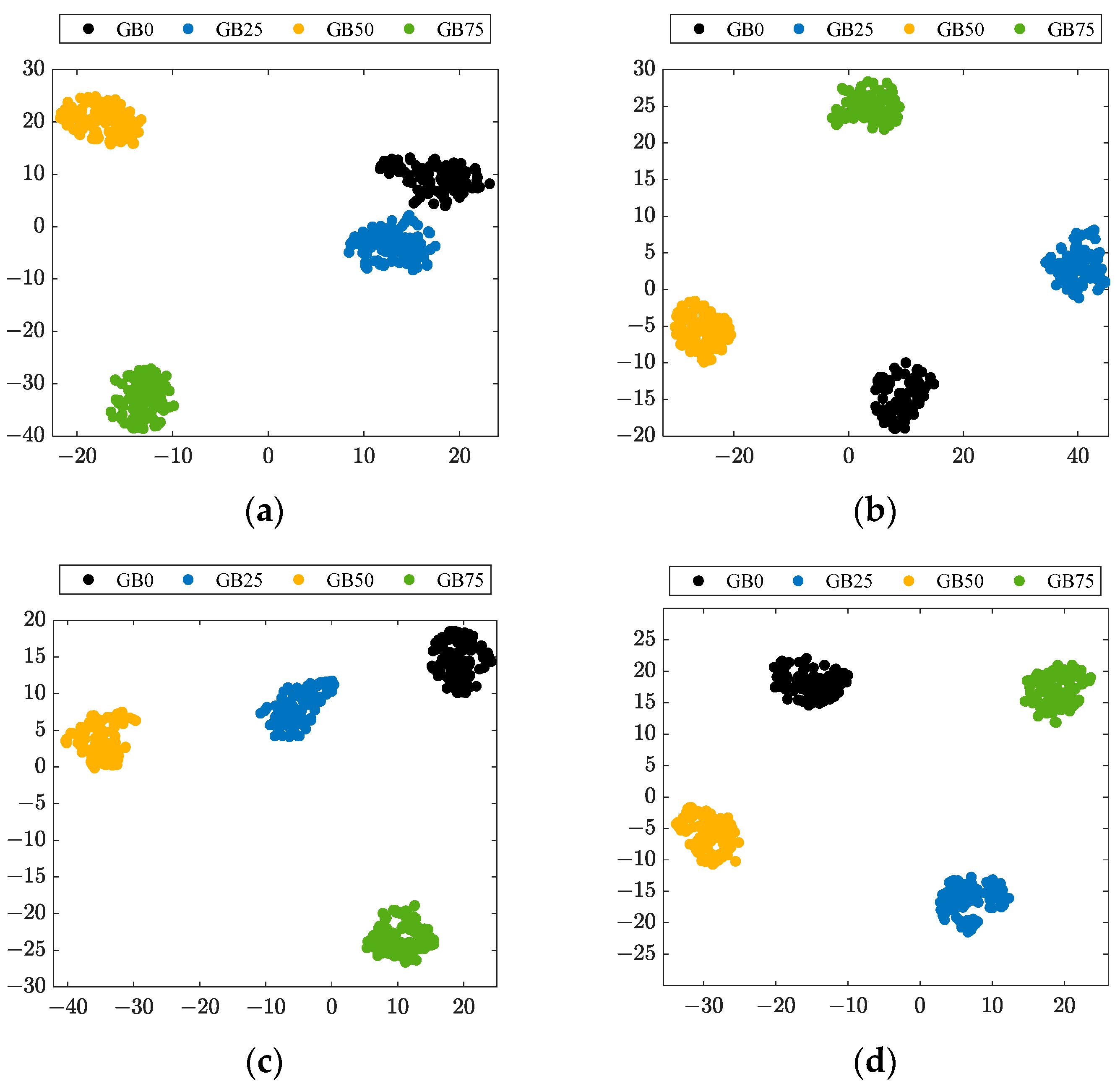
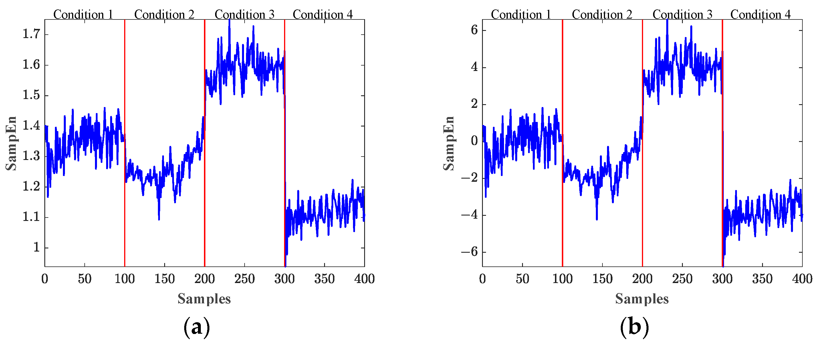
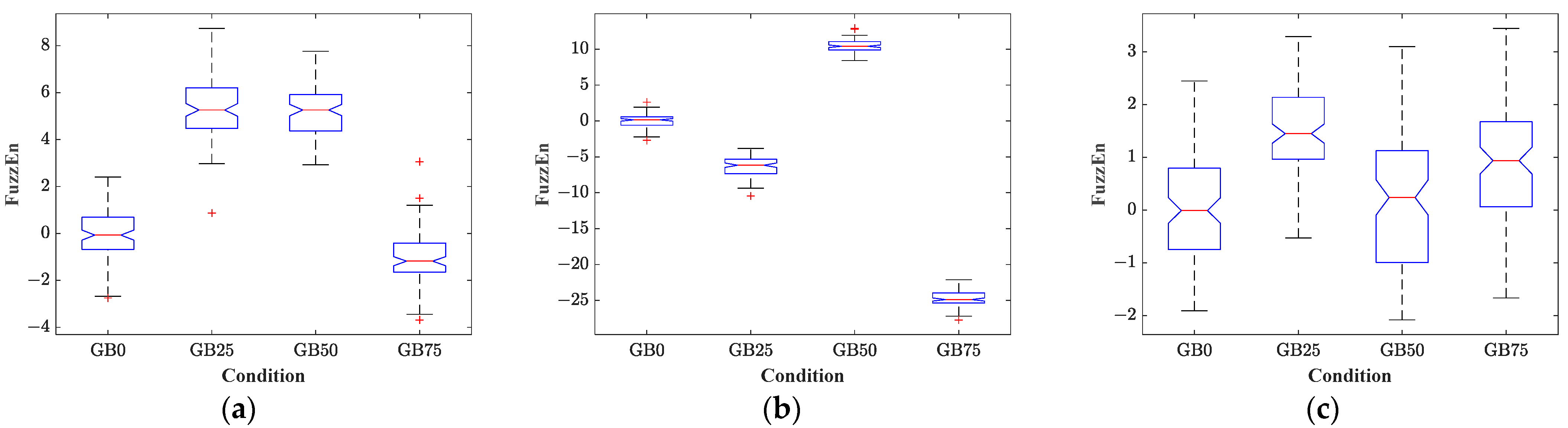
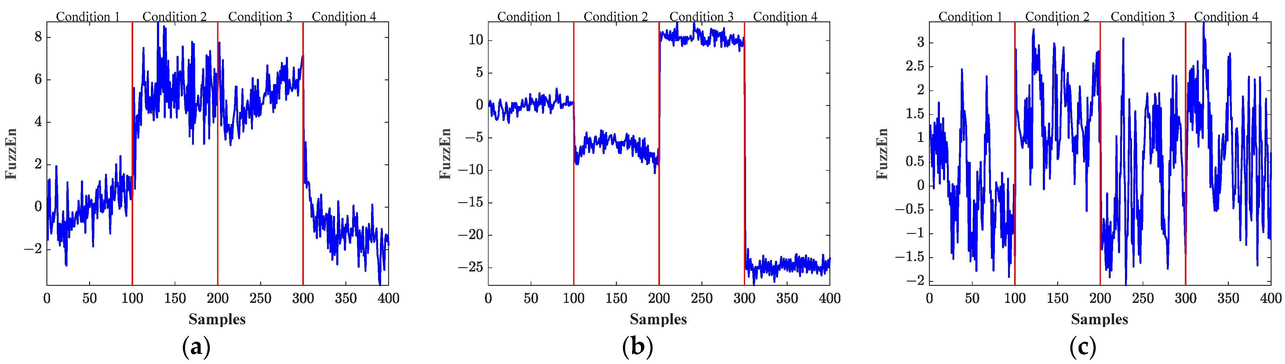
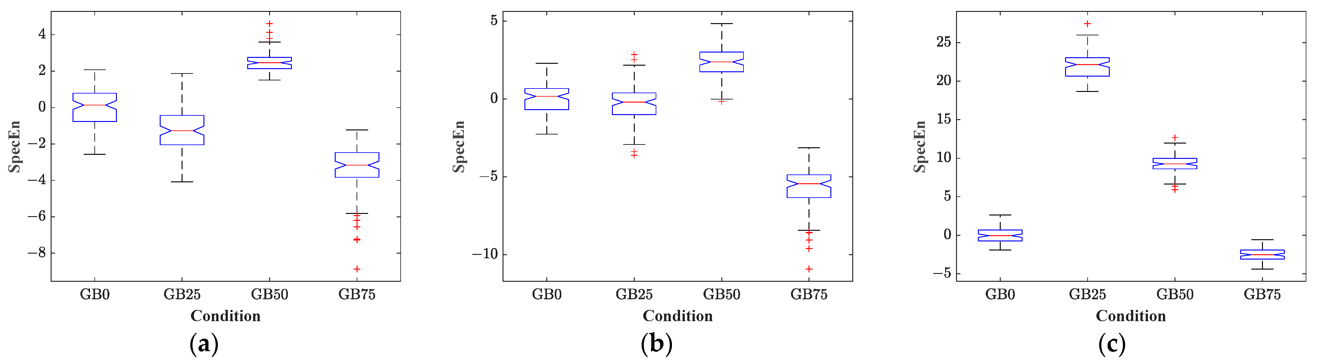
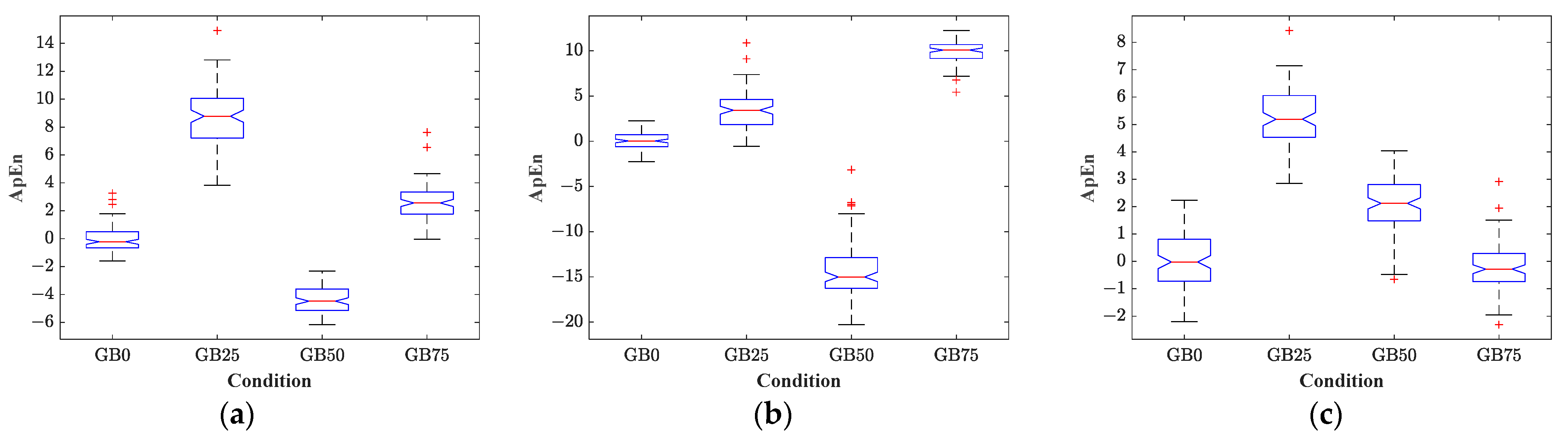
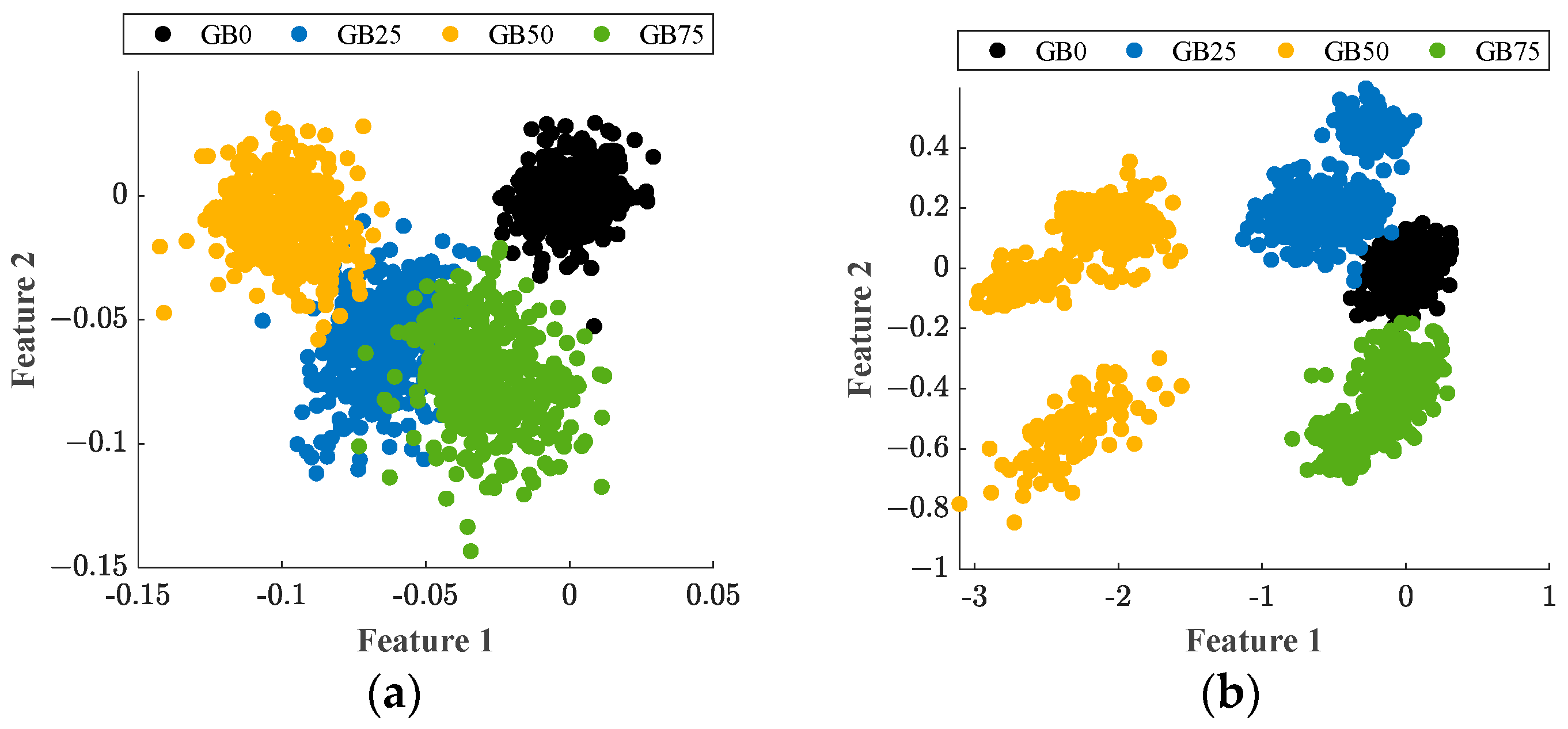
5.1. Entropy Analysis for Detecting Faults in the GB

According to the explanation of the second stage of the methodology and the diagram observed in Figure 2, the two vibration signals subject to further processing are the V y and the V z , and the stator’s current signature is C 1 . Thus, the six entropy features previously mentioned are computed from each one of these signals according to the explanation of the third stage of the proposed methodology. Hence, as a result, three characteristic feature matrices are obtained, which are V y , V z , and C 1 ; each feature matrix has a dimension of 6 × 100 where the columns represent the six entropy features and the rows belong to each one of the segmented parts of V y ,   V z , and C 1 , respectively. In addition, the characteristic features matrices are obtained to generate a consecutive set of samples (100 samples) for each one of the entropy features; accordingly, due to the four different supply electrical frequencies of operation used to carry out the experimentation for each condition twelve characteristic feature matrices are computed; for example, for the gearbox in healthy condition (GB0), the matrices obtained are V y G B 0 @ 5 H z , V z G B 0 @ 5 H z , C 1 G B 0 @ 5 H z , V y G B 0 @ 15 H z , V z G B 0 @ 15 H z , C 1 G B 0 @ 15 H z , V y G B 0 @ 50 H z , V z G B 0 @ 50 H z , C 1 G B 0 @ 50 H z , V y G B 0 @ 60 H z , V z G B 0 @ 60 H z , and C 1 G B 0 @ 60 H z . Once all the feature matrices are computed for all the considered conditions, the feature normalization is carried out by normalizing each entropy feature to zero mean and unit variance; this procedure plays a key role in condition monitoring strategies since it leads to improving the model performance and allows to ensure convergence. Figure 3a shows the qualitative visual representation of the SampEn feature without normalization that is estimated directly from the V z signal for all conditions of uniform wear (GB0, GB25, GB50, and GB75). On the other hand, Figure 3b also shows the SampEn feature after applying the normalization procedure. As observed, the amplitude scale of the vertical axis in Figure 3b is significantly higher than the amplitude scale of the vertical axis in Figure 3a. This particular difference between amplitude scales in vertical axes may produce a significant increase in terms of accuracy and performance when normalized features are used to produce the fault assessment. The normalization procedure is applied to all feature matrices for all studied conditions and normalized feature matrices are then obtained ( N V y , N V z , and N C 1 ); for example, for the GB0 condition, the normalized matrices obtained are N V y G B 0 @ 5 H z , N V z G B 0 @ 5 H z , and N C 1 G B 0 @ 5 H z , when the kinematic chain operates at 5 Hz for the signals V y , V z , and C 1 , respectively.
Afterward, the normalized entropy features are then analyzed using two different approaches with the aim of determining their capabilities for being included in diagnosis strategies applied to the detection and identification of faults in kinematic chains. Thus, the KW test and the FDS are applied over the previously normalized features; hence, the KW test is first applied to each entropy feature for all studied conditions in the GB. Thereby, Equation (12) is used to carry out the KW test, for the conditions tested in the GB the number of classes is defined as C = 4 , with a total number of samples N = 400 for all classes with n i = 100 samples per class.
Specifically, for each available signal and each operating condition, the KW test is individually applied to each entropy feature of the normalized feature matrices N V y , N V z , and N C 1 , i.e., the KW test leads to achieving twelve numerical p-values for only one entropy feature for the signals V y , V z , and C 1 for all GB conditions. This test is carried out to determine whether a group of data points (samples) comes from the same population. In this regard, the quantitative metric known as p-value may depict the level of distinction between the assessed conditions (classes); in particular, p-values smaller than 0.05 mean that there exist statistically significant differences between analyzed classes. Consequently, Table 2 summarizes the p-values achieved during the KW test applied to the corresponding normalized entropy features estimated from signals V y , V z , and C 1 for the conditions GB0, GB25, GB50, and GB75 that are tested in the GB for all the supply electrical frequencies of operation 5 Hz, 15 Hz, 50 Hz, and 60 Hz. As appreciated in Table 2, most of the entropy features for the signals V y , V z , and C 1 produce p-values smaller than 0.05 demonstrating that these features have significant information to differentiate between the analyzed conditions. Specifically, most of the p-values obtained during the test are represented on a scale that varies from 1 × 10 13 to 1 × 10 81 , which theoretically can be taken into account as zero.
The KW test also allows to obtain boxplots with the aim of comparing the data distribution of the classes under analysis; Figure 4a–c show the boxplots for the FuzzEn feature computed from the signals V y , V z , and C 1 for all conditions tested in the GB when the kinematic chain operates at 60 Hz, respectively. The corresponding p-values computed for these boxplots are 7.10 × 10 67 , 9.17 × 10 81 , and 1.92 × 10 22 , respectively, and the labels in the horizontal axes directly indicate the conditions tested in the GB. On the other side, the horizontal red line inside the boxes represents the median of the tested conditions, whereas the red symbols ‘+’ are samples detected as outliers. Accordingly, based on the KW test, it can be assumed that the FuzzEn feature provides statistically significant information to discriminate between assessed conditions in the GB, and this assertion is supported by the achieved p-values, which are smaller than 0.05. In fact, the FuzzEn estimated from the signal V z is the most representative because the medians of all classes (horizontal red lines inside the boxes) are vertically separated from each other, avoiding the overlapping between the considered conditions. In its counterpart, the FuzzEn estimated from signals V y and C 1 also produce p-values smaller than 0.05, but their corresponding boxplots show a slight overlapping; that is, in Figure 4a, medians of conditions GB25 and GB50 appear horizontally aligned and in Figure 4c there is not a considerable separation between the medians of all conditions. Finally, the quantitative representation of the FuzzEn feature estimated from signals V y , V z , and C 1 when the kinematic chain operates at 60 Hz is shown in Figure 5a–c, respectively. These quantitative values belong to the normalized FuzzEn for the four conditions (100 samples per condition). As appreciated, there exists a clear difference between the values of FuzzEn in Figure 5b for each assessed condition, whereas the values of FuzzEn in Figure 5a only present different amplitudes for the GB0, GB25, and GB50 conditions, and the values of FuzzEn in Figure 5c do not show considerable changes between all conditions.
Following the proposed method, the entropy features are also analyzed through the FDS approach to determine their discriminant properties for distinguishing between classes. Hence, for each one of the three signals and each supply electrical frequency of operation in the VFD, the analysis based on FDS is individually carried out over each entropy feature as follows:
(i)
An entropy feature from the normalized feature matrices N V y , N V z , and N C 1 is selected, such as, for example, the FuzzEn.
(ii)
When analyzing the studied conditions in the GB, firstly, the samples of the FuzzEn feature from the GB0 condition are compared to the samples of the FuzzEn feature from the GB25 condition by using (13)–(15). As a result, a discriminant ratio ( F S r ) is computed, which measures the linear separation between the GB0 and GB25 conditions.
(iii)
The previous step is repeated for the same entropy feature (i.e., FuzzEn) until all faulty conditions (GB25, GB50, and GB75) are iteratively faced with the healthy condition (GB0).
(iv)
Another entropy feature is selected and steps (II) and (III) are performed; over the new entropy feature, the procedure is applied to all available entropy features.
Thereby, Table 3 summarizes the F S r scores achieved by applying the FDS analysis to each normalized entropy feature estimated from the signals V y , V z and C 1 for the operating supply frequencies 5 Hz and 15 Hz, whereas Table 4 summarizes the F S r scores for the operating supply frequencies 50 Hz and 60 Hz. Theoretically, values of F S r higher than 1 are associated with features that provide significant discriminant information to separate the classes under analysis; that is, entropy features that produce F S r > 1 ensures the separability of classes. Thus, for the normalized values of FuzzEn features presented in Figure 5a, the F S r scores are 26.65, 41.89, and 0.06 when facing GB0 vs. GB25, GB0 vs. GB50, and GB0 vs. GB75, respectively; these F S r scores mean that the FuzzEn estimated from V y signal has the capability to distinguish the GB0 condition from GB25 and GB50 conditions, but not from the GB75 condition. On the other hand, for the normalized FuzzEn feature of Figure 5b, the computed F S r scores are 46.41, 971.21, and 23,643.02; these values describe a high capability of the FuzzEn feature estimated from the V z signal for separating any of the faulty conditions (GB25, GB50, and GB75) from the healthy one (GB0). Likewise, the F S r scores for the normalized FuzzEn feature, estimated from the C 1 signal, and shown in Figure 5c are 0.52, 0.00, and 0.03, respectively. Hence, these values depict a lack of meaningful information to separate the healthy condition from the faulty ones.
In addition, to complement the proposed signal entropy analysis for the assessment of uniform wear in the GB, Figure 6a–c present the boxplots for the normalized SpecEn feature estimated from the signals V y , V z , and C 1 . The KW test applied to these normalized values leads to obtaining p-values equal to 4.64 × 10 71 , 2.52 × 10 69 , and 5.01 × 10 80 for each corresponding signal when the kinematic chain operates at 60 Hz. Likewise, the most relevant F S r scores are computed for the C 1 signal with values about 3460.57, 246.86, and 3.67 when facing GB0 vs. GB25, GB0 vs. GB50, and GB0 vs. GB75, correspondingly. Also, another important F S r score is calculated for the V z   signal when comparing GB0 vs. GB75 conditions, and such an F S r score is equal to 30.72. Therefore, it should be highlighted that there exists a relationship between higher values in the F S r score and the vertical separation of medians in the boxplots. On the other side, it is also probable that a specific feature computed from a particular signal does not provide sufficient information for distinguishing between different conditions, but another feature may provide enough information to carry out the class separation. In this regard, Figure 7a–c present the boxplots obtained for the normalized ApEn feature estimated from the signals V y , V z , and C 1 when the kinematic chain operates at 60 Hz, separately; their associated p-values are 6.74 × 10 79 , 1.74 × 10 78 , and 3.10 × 10 66 . As well, the computed F S r scores for the V y signal are 30.91, 1.17, and 43.97, and, for the V z signal they are 29.19, 116.48, and 1.05. In the case of the C 1 signal, the corresponding scores are 1.87, 384.40, and 0.00 when the healthy condition is faced with each faulty condition. It is worth mentioning that the ApEn feature provides meaningful information for assessing different severities of uniform wear in the GB.
Additionally, during the entropy signal analysis for detecting uniform wear in a GB, it can be noticed that the consideration of a single feature may not contain enough discriminant information to separate all the assessed conditions; in this regard, the combination of different entropy features may increase the capabilities of condition monitoring strategies to perform the fault assessment. Hence, to validate this assertion, the combination of three entropy features is tested and evaluated under the FDS analysis; that is, due to each tested condition characterized by 18 entropy features (6 entropy features per signal, V y , V z , and C 1 as summarized in the Table 5), there are C 3 18 = 816 possible combinations to be analyzed using Equations (13)–(15). Also, during this analysis, the GB0 condition is individually faced against the GB25, GB50, and GB75 conditions for each operating condition of the kinematic chain (5 Hz, 15 Hz, 50 Hz, and 60 Hz), the resulting F S r scores are ranked in descending order and the first three ranked F S r values are considered the most relevant. Table 6 summarizes the first three ranked F S r values: as observed, any of the resulting combinations produce F S r > 11 , which ensures the separability of classes; the smallest F S r scores are computed when GB0 is faced with GB25 when the kinematic chain operates at 5 Hz. Meanwhile, the highest F S r scores are computed also when GB0 is faced with GB25 when the kinematic chain operates at 50 Hz.
In order to validate that the combination of entropy features may improve the capability of condition monitoring strategies to perform the fault assessment, the t-distributed stochastic neighbor embedding (t-SNE) is used to obtain the visual representation of the best-ranked features (last row in Table 6) into a two-dimensional (2D) space. As a result, Figure 8a, Figure 8b, Figure 8c, and Figure 8d show the 2D visual representation of the data distribution for the best-ranked features resulting from evaluating all possible combinations ( C 3 18 = 816 ) by the FDS when the kinematic chain operates at 5 Hz, 15 Hz, 50 Hz, and 60 Hz, respectively. It should be highlighted that all conditions of uniform wear (GB0, GB25, GB50, and GB75) tested in the GB appear separated from each other for any of the supply electrical frequencies of operation; thus, the use of entropy features estimated from vibration signals and stator current signatures can lead to the accurate assessment of faults in rotating machines like GBs.

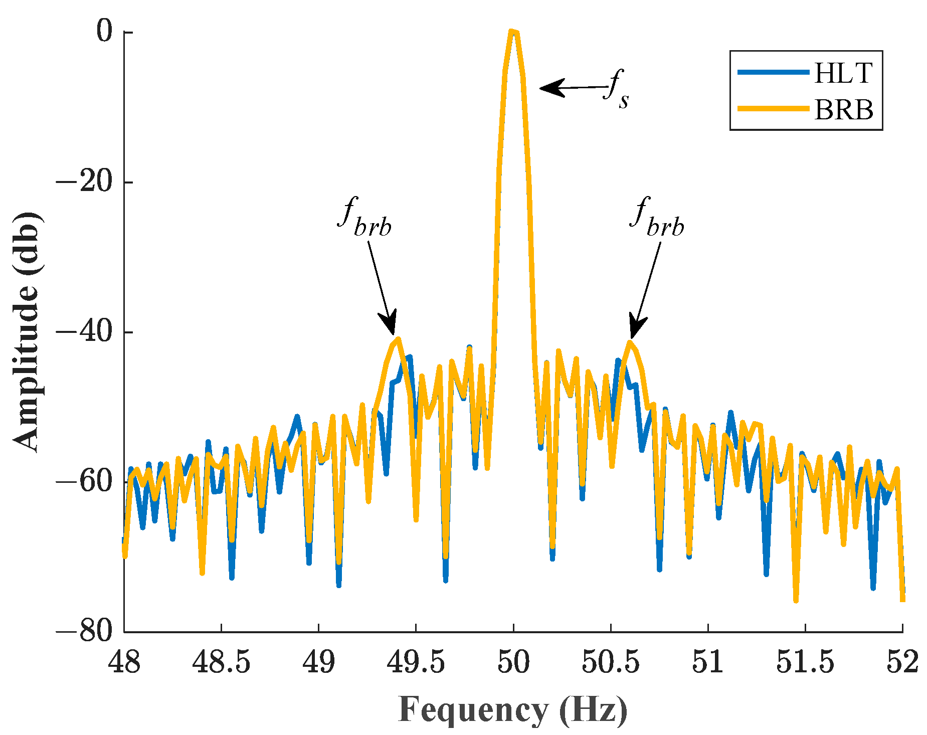
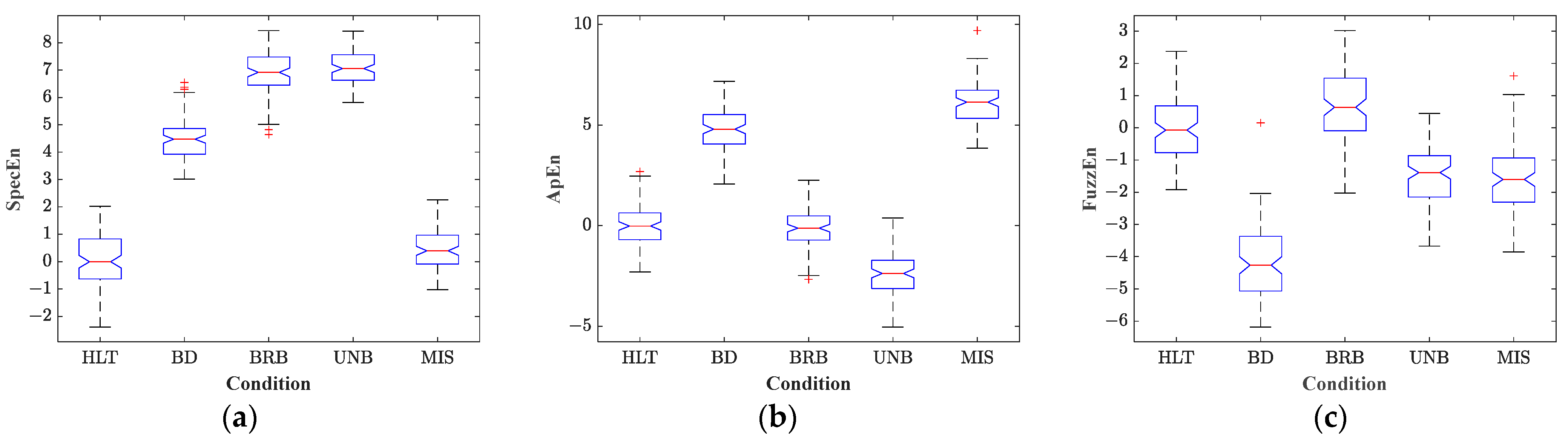
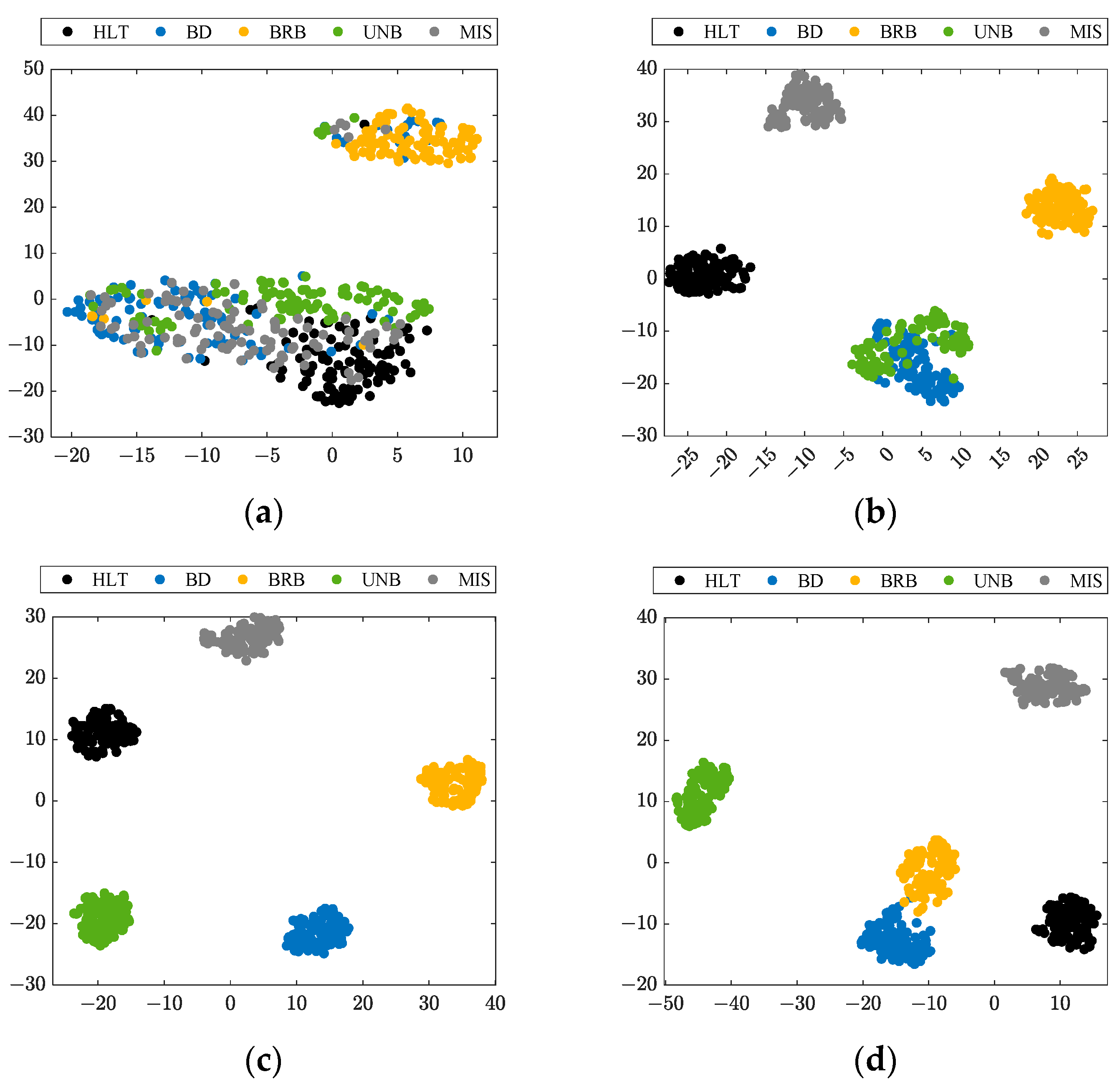
5.2. Entropy Analysis for Detecting Faults in the IM

Successively, as mentioned in the Section 3, the proposed entropy signal analysis is also applied to another dataset, which is also composed of vibration signals and stator current signatures, but, acquired during the evaluation of different faulty conditions such as HLT, BD, BRB, UNB, and MIS in an IM linked to a kinematic chain that operates at four different supply electrical frequencies of operation such as 5 Hz, 15 Hz, 50 Hz, and 60 Hz. The entropy analysis is applied to the same three signals V y , V z , and C 1 ; thus, these signals are equally segmented, and then the proposed set of entropy features from each segmented part is estimated. As a result, similarly to the analysis in the GB, three characteristic feature matrices are obtained, V y , V z , and C 1 , with a dimension of 6 × 100 . Now, in this case, for the IM under the BRB condition, the following twelve matrices— V y B R B @ 5 H z , V z B R B @ 5 H z , C 1 B R B @ 5 H z , V y B R B @ 15 H z , V z B R B @ 15 H z , C 1 B R B @ 15 H z , V y B R B @ 50 H z , V z B R B @ 50 H z , C 1 B R B @ 50 H z , V y B R B @ 60 H z , V z B R B @ 60 H z , and C 1 B R B @ 60 H z —are obtained for all frequencies. Afterward, the normalization procedure is carried out and the normalized feature matrices are generated, N V y , N V z and N C 1 , where entropy features have zero mean and unit variance, i.e., for the BRB condition, the matrices N V y B R B @ 5 H z , N V z B R B @ 5 H z , and N C 1 B R B @ 5 H z are obtained when the kinematic chain operates at 5 Hz.
Once the normalization of all the feature matrices is performed, the KW test is carried out using Equation (12); thereby, for the conditions tested in the IM, the number of classes is defined as C = 5 , with a total number of samples N = 500 , for all classes with n i = 100 samples per class. Table 7 summarizes the resulting p-values; as observed, most of the p-values are smaller than 0.05, which describes statistically significant differences between the analyzed classes. In fact, most of the achieved p-values are represented on a scale that varies from 1 × 10 9 to 1 × 10 97 ; ideally, these values can be understood as zero. On the other hand, Figure 9a–c show the resulting boxplots achieved for the SpecEn feature estimated from V y , the ApEn feature estimated from V z , and the FuzzEn feature estimated from C 1 , respectively, when the kinematic chain operates at 50 Hz. As appreciated, each one of the entropy features provides statistically significant information to separate specific conditions; that is, SpecEn can separate the HLT condition from BD, BRB, and UNB, but produce a slight overlapping with the MIS condition. Meanwhile, the ApEn has the capability of separating the HLT condition from BD, UNB, and MIS but not from the BRB condition. At last, the FuzzEn also separates the HLT condition from BD, UNB, and MIS; meanwhile, a slight overlapping is produced with the BRB condition.
Successively, the FDS analysis is performed by using Equations (13)–(15), with the aim of evaluating the discriminant properties of each normalized entropy feature and distinguishing between the conditions tested in the IM. Hence, Table 8 summarizes the F S r scores achieved when the HLT condition is faced with each faulty condition and the supply electrical frequencies of operation used in the kinematic chain are 5 Hz and 15 Hz. Meanwhile, Table 9 summarizes the F S r scores obtained when the kinematic chain operates at 50 Hz and 60 Hz. As appreciated in Table 8, only a few entropy features for some specific signals lead to the production of F S r scores higher than 1 for the operating frequency of 5 Hz, whereas for 15 Hz, most of the F S r scores are higher than 1; thereby, it could be possible to obtain misclassifications when F S r scores smaller than 1 are produced. On the other hand, as depicted in Table 9, the values of F S r scores are higher than 1 for almost all the entropy features for the three signals, and F S r > 1 may ensure the separability of assessed conditions. As previously stated, a specific entropy feature may not provide sufficient information to separate the healthy condition from the faulty ones. In this sense, C 3 18 = 816 possible combinations of three entropy features are also evaluated using Equations (13)–(15), accordingly; during the analysis, the HLT condition is faced with the BD, BRB, UNB, and MIS conditions for each operating supplying frequency of the kinematic chain (5 Hz, 15 Hz, 50 Hz, and 60 Hz). Table 10 summarizes the first three ranked F S r values, as appreciated, and only the F S r scores achieved when the HLT condition is faced with the MIS condition (operating at 5 Hz) produce F S r < 1 , whereas the reaming F S r scores lead to F S r > 1 . Finally, the t-SNE is used to obtain the visual representation of the best-ranked features (last row in Table 10) in a 2D space; thus, Figure 10a–d show the data distributions for the best-ranked features when the kinematic chain operates at 5 Hz, 15 Hz, 50 Hz, and 60 Hz, respectively. It must be emphasized that all tested conditions in the IM (HLT, BD, BRB, UNB, and MIS) appear separated from each other for the operating frequencies of 50 Hz and 60 Hz (Figure 10c,d). Meanwhile, in Figure 10b, all the faulty conditions are separated from the HLT one when the kinematic chain operates at 15 Hz; nevertheless, an unexpected overlapping is produced between BD and UNB conditions. Unfortunately, in Figure 10a, the HLT, BD, UNB, and MIS conditions appear to overlap between them when the kinematic chain operates at 5 Hz, and only the BRB condition tries to be separated from the other conditions. Therefore, it is worth mentioning that the use of entropy features estimated from vibration signals and stator current signatures can lead to the accurate diagnosis of faults like BD, BRB, UNB, and MIS in IMs; however, the assessment of faults in IMs through entropy features can be sensitive to the rotating speed, specifically, at high operating frequencies (50 Hz and 60 Hz), an accurate assessment of faults is performed, but some limitations are presented during the fault diagnosis at an extremely low operating frequency (5 Hz).

5.3. Comparison versus Classical Approaches

Finally, a comparison with classical approaches is performed to highlight that entropy features provide meaningful information to carry out the detection of faults in GBs and IMs; in this regard, the estimation of frequency spectra through the FFT has represented a suitable diagnosis tool for detecting the occurrence of faults in rotating machinery. For example, the detection of problems associated with rotor bars in IMs is commonly addressed due to the unbalance of the air-gap magnetic flux leading to the generation of a fault-related frequency component around the supply frequency ( f s ) in the frequency spectrum at f b r b = 1 ± 2 k s f s ,   k + 1,2 , 3 , . Nevertheless, the detection of faults based on the analysis of frequency spectra requires prior knowledge and expertise since the calculation of fault-related frequency components depends on additional variables such as the per-unit slip ( s = n s n r / n s ), which, in turn, is in terms of the synchronous ( n s ) and rotating rotor speed ( n r ). Figure 11 shows the obtained frequency spectra by applying the FFT technique to the stator current signatures acquired when the IM is tested under the HLT and BRB conditions at 50 Hz as the supply electrical frequency of operation, as observed, the spectrum associated with the BRB condition produces the f b r b components appearing at 49.4 Hz and 50.59 Hz for a slip of around 1.5%. Although faults like BRBs introduce modifications in specific fault-related frequency components, the accuracy of the diagnosis depends on the technician’s knowledge. Hence, the analysis of changes and trends through the estimation of entropy features represents a suitable option to achieve the occurrence of any fault in rotating machinery like IMs or GBs.
On the other hand, DDA can be successfully applied for detecting and identifying faults in rotating machines; however, the performance achieved by these approaches depends on two main stages where a set of fault-related features is estimated and then subjected to a reduction procedure. That is, the statistical features such as RMS value, Standard Deviation, Kurtosis, Skewness, Shape Factor, and Latitude factor are commonly computed from raw signals aiming to model trends and changes; meanwhile, dimensionality reduction techniques such as PCA and/or LDA are used to compress and transform an original dataset into a 2D feature space. Consequently, to validate that the entropy features studied in this work provide significant information for fault diagnosis methodologies, the aforementioned statistical features have been computed from the raw signals V y , V z and C 1 for all tested conditions (GB0, GB25, GB50, and GB75) in the GB under all operating frequencies (5 Hz, 15 Hz, 50 Hz, and 60 Hz), and then are subjected to a reduction procedure using the LDA technique. Figure 12a shows the resulting 2D projection where it is possible to observe four main clusters representing the assessed conditions in the GB; unfortunately, the statistical features lead to overlapping between all faulty conditions. Additionally, to compare the performance between statistical features and entropy features, the entropy features studied in this work are also subjected to the reduction procedure by means of the LDA technique. Figure 12b presents the resulting 2D projection where an improvement between the separability of all considered conditions is obtained. It should be mentioned that for both sets of features (statistical and entropy), the reduction procedure has been applied to all samples of all studied conditions under all tested frequencies. Thereby, the obtained results support the use of entropy features as a part of condition monitoring methodologies for the detection and identification of faults that can occur in rotating elements like GBs and IMs.
Finally, Table 11 presents the most important highlights obtained during the comparison between the classical frequency analysis (performed by the FFT) and by comparing DDA in front of the entropy analysis performed in this work. In fact, it can be emphasized that the most critical issue is associated with prior knowledge and expertise for detecting those fault-related frequency components in a frequency spectrum; meanwhile, the use of entropy features and dimensionality reduction techniques, such as LDA, leads to improve the diagnosis outcome. On the other hand, Table 12 summarizes the highlights of the comparison between the entropy features analysis versus classical statistical features, both used in a DDA using the LDA technique, and the estimation of statistical time domain features is a suitable option to characterize trends and changes in time domain signals with an appropriate trade-off between simplicity and quickly responses; however, the obtained results demonstrate that entropy features significantly improve the assessment of faults regardless of the operating condition.

6. Conclusions

In this work, an analysis of entropy-based features was performed with the objective of identifying changes and trends produced by the unexpected occurrence of faults in a kinematic chain. Certainly, the proposed analysis is applied to vibration signals and stator current signatures acquired from real laboratory experiments, where different severities of uniform wear are tested in a GB and five different faulty conditions are tested in an IM. There are some important aspects that must be highlighted: the first one is that the calculation of the six proposed entropy features from available vibrations and stator currents leads to a high-performance characterization to assess the occurrence of faults in both GB and IM linked in a kinematic chain that operates at different supply electrical frequencies of operation. Indeed, each different condition under study produces different amplitude values during the calculation of entropy features; thus, any variation obtained in regard to the healthy condition is produced due to the occurrence of an undesirable faulty condition. The second aspect to be highlighted is that, in the analysis of entropy features using the KW test and the FDS technique, both approaches allow us to determine whether the proposed entropy features have statistically significant information for distinguishing between different conditions (classes). Certainly, through boxplots resulting from the KW test, it can be inferred when data points of the analyzed conditions can be separated from each other where the separation between classes is related to the vertical separation that appears between medians in the boxplots. On the other hand, it is demonstrated that overlapping problems are avoided when the values of F S r scores are higher than 1; additionally, it has been proved that the combination of entropy features contributes to a better separation between assessed conditions. The final aspect is that the use of entropy features provides significant information to perform the fault assessment for the detection of different severities of uniform wear in a GB regardless of the rotating frequency; on the contrary, when entropy features are applied to the diagnosis of faults in IMs, it may be possible to produce accurate detection of faults whether the IM operates at high supply frequencies but a lack of discriminant capabilities is present at extremely low operating frequencies. Thus, from the experimental tests, it can be concluded that entropy features have the advantage of providing wide energy behavior into a measured signal and, therefore, most of the indicators analyzed provided useful discriminatory information of the conditions; thus, the feature values were robust and consistent. This way, a question appears: why and when should the entropy-based features be used? The answer is that they can be applied in systems under unfavorable conditions like low values of the load (where most of the proposed approaches present difficulties for the diagnosis), also with different types of faults, not necessarily related to the bearing defects, like unbalance, misalignment, broken rotor barks, and gear wear. Thereby, entropy features represent a suitable option to be implemented as a part of condition monitoring strategies for the detection and identification of faults in different elements involved in a kinematic chain such as GBs and IMs. Future work should consider the combination of techniques in which entropy-based features can be exploited for diagnosing faults in non-stationary signals for combined faults, or even under unfavorable noise conditions combined with variable operating conditions.

Author Contributions

Conceptualization, D.A.E.-O. and R.d.J.R.-T.; Data Curation, D.A.E.-O. and R.d.J.R.-T.; Formal Analysis, J.J.S.-D. and R.d.J.R.-T.; Funding Acquisition, A.Y.J.-C.; Investigation, A.Y.J.-C. and R.d.J.R.-T.; Methodology, A.Y.J.-C., J.J.S.-D. and D.A.E.-O.; Project Administration, A.Y.J.-C. and R.d.J.R.-T.; Resources, A.Y.J.-C.; Supervision, A.Y.J.-C., J.J.S.-D. and R.d.J.R.-T.; Validation, J.J.S.-D.; Visualization, D.A.E.-O. and R.d.J.R.-T.; Writing—Original Draft, J.J.S.-D. and D.A.E.-O.; Writing—Review and Editing, A.Y.J.-C. and J.J.S.-D. All authors have read and agreed to the published version of the manuscript.

Funding

This project has been partially supported by the Universidad Autonoma de Querétaro through “Fondo para el Desarrollo del Conocimiento” (FONDEC-UAQ-2022) under project number 20205007071601, and partially by the CONAHCyT 487599, 331141, 558497 and 120260 SNII grants.

Data Availability Statement

Publicly available datasets were analyzed in this study. These data can be found here: [https://grouper.ieee.org/groups/1159/3/docs.html, (accessed on 14 April 2024)].

Conflicts of Interest

The authors declare no conflicts of interest.

References

  1. Sardar, M.U.; Vaimann, T.; Kütt, L.; Kallaste, A.; Asad, B.; Akbar, S.; Kudelina, K. Inverter-Fed Motor Drive System: A Systematic Analysis of Condition Monitoring and Practical Diagnostic Techniques. Energies 2023, 16, 5628. [Google Scholar] [CrossRef]
  2. Drakaki, M.; Karnavas, Y.L.; Tzionas, P.; Chasiotis, I.D. Recent Developments Towards Industry 4.0 Oriented Predictive Maintenance in Induction Motors. Procedia Comput. Sci. 2021, 180, 943–949. [Google Scholar] [CrossRef]
  3. Torrent, M.; Blanqué, B.; Monjo, L. Replacing Induction Motors without Defined Efficiency Class by IE Class: Example of Energy, Economic, and Environmental Evaluation in 1.5 kW—IE3 Motors. Machines 2023, 11, 567. [Google Scholar] [CrossRef]
  4. Zhang, J.; Wang, P.; Gao, R.X.; Sun, C.; Yan, R. Induction Motor Condition Monitoring for Sustainable Manufacturing. Procedia Manuf. 2019, 33, 802–809. [Google Scholar] [CrossRef]
  5. Gangsar, P.; Tiwari, R. Signal Based Condition Monitoring Techniques for Fault Detection and Diagnosis of Induction Motors: A State-of-the-Art Review. Mech. Syst. Signal Process. 2020, 144, 106908. [Google Scholar] [CrossRef]
  6. Workineh, T.G.; Jember, Y.B.; Kassie, A.T. Evaluation of Intelligent PPI Controller for the Performance Enhancement of Speed Control of Induction Motor. Sci. Afr. 2023, 22, e01982. [Google Scholar] [CrossRef]
  7. Chen, C.; Yuan, Y.; Sun, W.; Zhao, F. Multivariate Multi-Step Time Series Prediction of Induction Motor Situation Based on Fused Temporal-Spatial Features. Int. J. Hydrog. Energy 2024, 50, 1386–1394. [Google Scholar] [CrossRef]
  8. Singh, G.; Anil Kumar, T.C.; Naikan, V.N.A. Efficiency Monitoring as a Strategy for Cost Effective Maintenance of Induction Motors for Minimizing Carbon Emission and Energy Consumption. Reliab. Eng. Syst. Saf. 2019, 184, 193–201. [Google Scholar] [CrossRef]
  9. Rangel-Magdaleno, J.; Peregrina-Barreto, H.; Ramirez-Cortes, J.; Cruz-Vega, I. Hilbert Spectrum Analysis of Induction Motors for the Detection of Incipient Broken Rotor Bars. Measurement 2017, 109, 247–255. [Google Scholar] [CrossRef]
  10. Kumar, S.; Mukherjee, D.; Guchhait, P.K.; Banerjee, R.; Srivastava, A.K.; Vishwakarma, D.N.; Saket, R.K. A Comprehensive Review of Condition Based Prognostic Maintenance (CBPM) for Induction Motor. IEEE Access 2019, 7, 90690–90704. [Google Scholar] [CrossRef]
  11. Mallik, S.; Mallik, K.; Barman, A.; Maiti, D.; Biswas, S.K.; Deb, N.K.; Basu, S. Efficiency and Cost Optimized Design of an Induction Motor Using Genetic Algorithm. IEEE Trans. Ind. Electron. 2017, 64, 9854–9863. [Google Scholar] [CrossRef]
  12. IEA. World Energy Outlook 2023—Analysis, International Energy Agency. Available online: https://www.iea.org/reports/world-energy-outlook-2023 (accessed on 28 February 2024).
  13. Bessous, N.; Sbaa, S.; Toumi, A. Experimental Investigation on Broken Rotor Bar Faults in Three Phase Induction Motors Using MVSA-FFT Method. In Proceedings of the 2018 6th International Conference on Control Engineering & Information Technology (CEIT), Istanbul, Turkey, 25–27 October 2018; pp. 1–7. [Google Scholar]
  14. Kompella, K.C.D.; Mannam, V.G.R.; Rayapudi, S.R. DWT Based Bearing Fault Detection in Induction Motor Using Noise Cancellation. J. Electr. Syst. Inf. Technol. 2016, 3, 411–427. [Google Scholar] [CrossRef]
  15. Jain, S.K.; Singh, S.N. Harmonics Estimation in Emerging Power System: Key Issues and Challenges. Electr. Power Syst. Res. 2011, 81, 1754–1766. [Google Scholar] [CrossRef]
  16. Chen, Z.; Liang, D.; Jia, S.; Yang, L.; Yang, S. Incipient Interturn Short-Circuit Fault Diagnosis of Permanent Magnet Synchronous Motors Based on the Data-Driven Digital Twin Model. IEEE J. Emerg. Sel. Top. Power Electron. 2023, 11, 3514–3524. [Google Scholar] [CrossRef]
  17. Bittencourt, A.C.; Saarinen, K.; Sander-Tavallaey, S.; Gunnarsson, S.; Norrlöf, M. A Data-Driven Approach to Diagnostics of Repetitive Processes in the Distribution Domain—Applications to Gearbox Diagnostics in Industrial Robots and Rotating Machines. Mechatronics 2014, 24, 1032–1041. [Google Scholar] [CrossRef]
  18. Rosa, T.E.; de Paula Carvalho, L.; Gleizer, G.A.; Jayawardhana, B. Fault Detection for LTI Systems Using Data-Driven Dissipativity Analysis. Mechatronics 2024, 97, 103111. [Google Scholar] [CrossRef]
  19. Jaen-Cuellar, A.Y.; Elvira-Ortiz, D.A.; Saucedo-Dorantes, J.J. Statistical Machine Learning Strategy and Data Fusion for Detecting Incipient ITSC Faults in IM. Machines 2023, 11, 720. [Google Scholar] [CrossRef]
  20. Wang, H.; Zheng, J.; Xiang, J. Online Bearing Fault Diagnosis Using Numerical Simulation Models and Machine Learning Classifications. Reliab. Eng. Syst. Saf. 2023, 234, 109142. [Google Scholar] [CrossRef]
  21. Das, O.; Bagci Das, D.; Birant, D. Machine Learning for Fault Analysis in Rotating Machinery: A Comprehensive Review. Heliyon 2023, 9, e17584. [Google Scholar] [CrossRef]
  22. Saucedo-Dorantes, J.J.; Jaen-Cuellar, A.Y.; Perez-Cruz, A.; Elvira-Ortiz, D.A. Detection of Inter-Turn Short Circuits in Induction Motors under the Start-Up Transient by Means of an Empirical Wavelet Transform and Self-Organizing Map. Machines 2023, 11, 958. [Google Scholar] [CrossRef]
  23. Arellano-Espitia, F.; Delgado-Prieto, M.; Martínez-Viol, V.; Saucedo-Dorantes, J.-J.; Osornio-Rios, R.A. Diagnosis Electromechanical System by Means CNN and SAE: An Interpretable-Learning Study. In Proceedings of the 2022 IEEE 5th International Conference on Industrial Cyber-Physical Systems (ICPS), Coventry, UK, 24–26 May 2022; pp. 1–6. [Google Scholar]
  24. Chen, M.; Shao, H.; Dou, H.; Li, W.; Liu, B. Data Augmentation and Intelligent Fault Diagnosis of Planetary Gearbox Using ILoFGAN Under Extremely Limited Samples. IEEE Trans. Reliab. 2023, 72, 1029–1037. [Google Scholar] [CrossRef]
  25. Ding, A.; Qin, Y.; Wang, B.; Cheng, X.; Jia, L. An Elastic Expandable Fault Diagnosis Method of Three-Phase Motors Using Continual Learning for Class-Added Sample Accumulations. IEEE Trans. Ind. Electron. 2023, 71, 7896–7905. [Google Scholar] [CrossRef]
  26. Choudhary, A.; Mian, T.; Fatima, S.; Panigrahi, B.K. Passive Thermography Based Bearing Fault Diagnosis Using Transfer Learning With Varying Working Conditions. IEEE Sens. J. 2023, 23, 4628–4637. [Google Scholar] [CrossRef]
  27. Akhtar, S.; Adeel, M.; Iqbal, M.; Namoun, A.; Tufail, A.; Kim, K.-H. Deep Learning Methods Utilization in Electric Power Systems. Energy Rep. 2023, 10, 2138–2151. [Google Scholar] [CrossRef]
  28. Liu, L.; Zhi, Z.; Zhang, H.; Guo, Q.; Peng, Y.; Liu, D. Related Entropy Theories Application in Condition Monitoring of Rotating Machineries. Entropy 2019, 21, 1061. [Google Scholar] [CrossRef]
  29. Li, Y.; Wang, X.; Liu, Z.; Liang, X.; Si, S. The Entropy Algorithm and Its Variants in the Fault Diagnosis of Rotating Machinery: A Review. IEEE Access 2018, 6, 66723–66741. [Google Scholar] [CrossRef]
  30. Li, Y.; Wang, X.; Si, S.; Huang, S. Entropy Based Fault Classification Using the Case Western Reserve University Data: A Benchmark Study. IEEE Trans. Reliab. 2020, 69, 754–767. [Google Scholar] [CrossRef]
  31. Huo, Z.; Martinez-Garcia, M.; Zhang, Y.; Yan, R.; Shu, L. Entropy Measures in Machine Fault Diagnosis: Insights and Applications. IEEE Trans. Instrum. Meas. 2020, 69, 2607–2620. [Google Scholar] [CrossRef]
  32. Leite, G.D.N.P.; Araújo, A.M.; Rosas, P.A.C.; Stosic, T.; Stosic, B. Entropy Measures for Early Detection of Bearing Faults. Phys. Stat. Mech. Its Appl. 2019, 514, 458–472. [Google Scholar] [CrossRef]
  33. Wan, S.; Zhang, X. Teager Energy Entropy Ratio of Wavelet Packet Transform and Its Application in Bearing Fault Diagnosis. Entropy 2018, 20, 388. [Google Scholar] [CrossRef]
  34. Fu, L.; Zhu, T.; Zhu, K.; Yang, Y. Condition Monitoring for the Roller Bearings of Wind Turbines under Variable Working Conditions Based on the Fisher Score and Permutation Entropy. Energies 2019, 12, 3085. [Google Scholar] [CrossRef]
  35. Ramteke, D.S.; Pachori, R.B.; Parey, A. Automated Gearbox Fault Diagnosis Using Entropy-Based Features in Flexible Analytic Wavelet Transform (FAWT) Domain. J. Vib. Eng. Technol. 2021, 9, 1703–1713. [Google Scholar] [CrossRef]
  36. Wang, X.; Si, S.; Li, Y. Hierarchical Diversity Entropy for the Early Fault Diagnosis of Rolling Bearing. Nonlinear Dyn. 2022, 108, 1447–1462. [Google Scholar] [CrossRef]
  37. Yuan, X.; Fan, Y.; Zhou, C.; Wang, X.; Zhang, G. Research on Twin Extreme Learning Fault Diagnosis Method Based on Multi-Scale Weighted Permutation Entropy. Entropy 2022, 24, 1181. [Google Scholar] [CrossRef] [PubMed]
  38. Cao, W.; Li, C.; Li, Z.; Wang, S.; Pang, H. Research on Low-Resistance Grounding Fault Line Selection Based on VMD with PE and K-Means Clustering Algorithm. Math. Probl. Eng. 2022, 2022, e5360302. [Google Scholar] [CrossRef]
  39. Kamiński, M.M. On Shannon Entropy Computations in Selected Plasticity Problems. Int. J. Numer. Methods Eng. 2021, 122, 5128–5143. [Google Scholar] [CrossRef]
  40. Altaf, S.; Soomro, M.W.; Mehmood, M.S. Fault Diagnosis and Detection in Industrial Motor Network Environment Using Knowledge-Level Modelling Technique. Model. Simul. Eng. 2017, 2017, e1292190. [Google Scholar] [CrossRef]
  41. Hassan, O.E.; Amer, M.; Abdelsalam, A.K.; Williams, B.W. Induction Motor Broken Rotor Bar Fault Detection Techniques Based on Fault Signature Analysis—A Review. IET Electr. Power Appl. 2018, 12, 895–907. [Google Scholar] [CrossRef]
  42. Feng, G.; Hu, N.; Mones, Z.; Gu, F.; Ball, A.D. An Investigation of the Orthogonal Outputs from an On-Rotor MEMS Accelerometer for Reciprocating Compressor Condition Monitoring. Mech. Syst. Signal Process. 2016, 76–77, 228–241. [Google Scholar] [CrossRef]
  43. Xu, Y.; Tang, X.; Feng, G.; Wang, D.; Ashworth, C.; Gu, F.; Ball, A. Orthogonal On-Rotor Sensing Vibrations for Condition Monitoring of Rotating Machines. J. Dyn. Monit. Diagn. 2021, 1, 29–36. [Google Scholar] [CrossRef]
  44. Ramteke, D.S.; Parey, A.; Pachori, R.B. A New Automated Classification Framework for Gear Fault Diagnosis Using Fourier–Bessel Domain-Based Empirical Wavelet Transform. Machines 2023, 11, 1055. [Google Scholar] [CrossRef]
  45. Jamil, M.A.; Khanam, S. Influence of One-Way ANOVA and Kruskal–Wallis Based Feature Ranking on the Performance of ML Classifiers for Bearing Fault Diagnosis. J. Vib. Eng. Technol. 2023. [Google Scholar] [CrossRef]
  46. Braga, J.A.P.; Andrade, A.R. Multivariate Statistical Aggregation and Dimensionality Reduction Techniques to Improve Monitoring and Maintenance in Railways: The Wheelset Component. Reliab. Eng. Syst. Saf. 2021, 216, 107932. [Google Scholar] [CrossRef]
  47. Hu, Q.; Si, X.-S.; Zhang, Q.-H.; Qin, A.-S. A Rotating Machinery Fault Diagnosis Method Based on Multi-Scale Dimensionless Indicators and Random Forests. Mech. Syst. Signal Process. 2020, 139, 106609. [Google Scholar] [CrossRef]
  48. Tripanpitak, K.; Viriyavit, W.; Huang, S.Y.; Yu, W. Classification of Pain Event Related Potential for Evaluation of Pain Perception Induced by Electrical Stimulation. Sensors 2020, 20, 1491. [Google Scholar] [CrossRef] [PubMed]
  49. Rostami, M.; Forouzandeh, S.; Berahmand, K.; Soltani, M. Integration of Multi-Objective PSO Based Feature Selection and Node Centrality for Medical Datasets. Genomics 2020, 112, 4370–4384. [Google Scholar] [CrossRef]
  50. Wan, H.; Wang, H.; Scotney, B.; Liu, J.; Ng, W.W.Y. Within-Class Multimodal Classification. Multimed. Tools Appl. 2020, 79, 29327–29352. [Google Scholar] [CrossRef]
Figure 1. General flow chart of the proposed methodology for analyzing the discriminant properties of six different entropy features extracted from raw signals of induction motors with fault conditions.
Electronics 13 01524 g001
Figure 2. Experimental test bench used for the evaluation of entropy signals as a fault-related feature.
Electronics 13 01524 g002
Figure 3. Qualitative representation of the SampEn feature estimated from the V z signal for all evaluated conditions in the gearbox (GB0, GB25, GB50, and GB75) when the kinematic chain operates at 60 Hz: (a) SampEn without normalization and (b) SamEn normalized to mean zero and unit variance.
Electronics 13 01524 g003
Figure 4. Boxplots achieved for the FuzzEn feature for the GB0, GB25, GB50, and GB75 conditions tested in the GB when the kinematic chain operates at 60 Hz; the boxplots for FuzzEn belong to the signals: (a) V y , (b) V z , and (c) C 1 .
Electronics 13 01524 g004
Figure 5. Quantitative representation of the estimated fuzzy entropy when evaluating the conditions of 0%, 25%, 50%, and 75% of uniform wear in the GB with an operating frequency of 60 Hz, the fuzzy entropy is estimated for (a) V y , (b) V z , and (c) C 1 .
Electronics 13 01524 g005
Figure 6. Boxplots of the estimated SpecEn feature when evaluating the GB0, GB25, GB50, and GB75 are tested in the GB with 60 Hz as operating frequency, the SpecEn is computed from signals: (a) V y , (b) V z , and (c) C 1 .
Electronics 13 01524 g006
Figure 7. Boxplots of the estimated ApEn feature when evaluating the GB0, GB25, GB50, and GB75 are tested in the GB and the kinematic chain operates at 60 Hz; the ApEn is computed from signals (a) V y , (b) V z , and (c) C 1 .
Electronics 13 01524 g007
Figure 8. Resulting projection achieved by applying the t-distributed stochastic neighbor embedding (t-SNE) to the ranked entropy features when the GB0 condition is faced with GB25, GB50 and GB75 for the kinematic chain operating at (a) 5 Hz, (b) 15 Hz, (c) 50 Hz and (d) 60 Hz.
Electronics 13 01524 g008
Figure 9. Boxplots obtained when evaluating the HLT, BD, BRB, UNB, and MIS conditions are evaluated in the IM and the kinematic chain operates at 50 Hz; the boxplots belong to (a) SpeEn feature estimated from V y , (b) ApEn feature estimated from V z , and (c) FuzzEn feature estimated from C 1 .
Electronics 13 01524 g009
Figure 10. Resulting projection achieved through the t-SNE during the evaluation of the best-ranked entropy features when the HLT condition in the IMs is faced with BD, BRB, UND, and MIS for the kinematic chain operating at (a) 5 Hz, (b) 15 Hz, (c) 50 Hz, and (d) 60 Hz.
Electronics 13 01524 g010
Figure 11. Frequency spectra obtained by applying the FFT technique over the acquired stator current signature when the conditions of HLT and BRB are tested in the IM and the supply frequency is fixed at 50 Hz.
Electronics 13 01524 g011
Figure 12. Resulting 2D projection obtained by applying the LDA technique to (a) statistical and (b) entropy features proposed in this work, both estimated from signals V y , V z , and C 1 . In the resulting projection, all evaluated frequencies have been considered (5 Hz, 15 Hz, 50 Hz, and 60 Hz).
Electronics 13 01524 g012
Table 1. Description of the different studied conditions tested in the GB and the IM.
Element under
Evaluation
Studied
Condition
Assigned
Label
DescriptionPicture
Gearbox
(GB)
GB with 0% of wearGB0The 4:1 GB is healthy, and the driven (72 teeth) and driver (18 teeth) gears are in perfect condition.
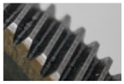
Electronics 13 01524 i001
GB with 25% of wearGB25Uniform wear is artificially induced to the driven gear until all teeth are worn within 25% of the original condition.
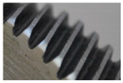
Electronics 13 01524 i002
GB with 50% of wearGB50Uniform wear is artificially induced to the driven gear until all teeth are worn within 50% of the original condition.
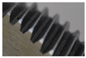
Electronics 13 01524 i003
GB with 75% of wearGB75Uniform wear is artificially induced to the driven gear until all teeth are worn within 75% of the original condition.Electronics 13 01524 i004
Induction motor (IM)Healthy IMHLTThe IM is healthy, and all the elements of the IM are in perfect condition.
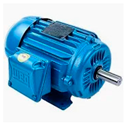
Electronics 13 01524 i005
Bearing defectBDThe outer bearing race in a 6205 bearing is artificially generated by drilling a through-hole with a 1.191 mm diameter.Electronics 13 01524 i006
Broken rotor barBRBA hole with 14 mm of depth is drilled in an IM rotor to completely break a rotor bar and to produce artificial damage.Electronics 13 01524 i007
UnbalanceUNBAn external mass (bolt) is attached to the rigid coupling that links the IM to the GB to produce an artificial unbalanced condition.
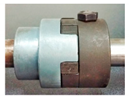
Electronics 13 01524 i008
MisalignmentMISThe free end of the IM is displaced to generate an angular misalignment of about 6 degrees.Electronics 13 01524 i009
Table 2. Quantitative p-value achieved during the KW test applied to the entropy features estimated from signals V y , V z , and C 1 for the conditions GB0, GB25, GB50, and GB75 tested in the GB.
Entropy FeaturesPhysical
Magnitude
Supply Electrical Frequencies of Operation
5 Hz15 Hz50 Hz60 Hz
SpecEn V y 0 0 0 0
V z 0 0 0 0
C 0 0 0 0
PermEn V y 0 0 0 0
V z 0 0 0 0
C 0 0 0 0
SampEn V y 0 0 0 0
V z 0 0 0 0
C 0 0 0 0
ApEn V y 0 0 0 0
V z 0 0 0 0
C 0 0 0 0
FuzzEn V y 0 0 0 0
V z 0 0 0 0
C 0 0 0 0
ReEn V y 0.00536 0.0716 0.0462 0.00522
V z 0.441 0.00230 0.0269 0.0218
C 0.318 0.448 0.217 0.664
Table 3. Quantitative Fisher score values achieved for the evaluation of the gearbox conditions (5 Hz and 15 Hz).
Supply Electrical Frequencies of Operation
5 Hz15 Hz
Entropy FeaturesPhysical
Magnitude
0% vs. 25%0% vs. 50%0% vs. 75%0% vs. 25%0% vs. 50%0% vs. 75%
SpecEn V y 0.13513.290.051.080.680.68
V z 0.0020.070.0013.05349.140.12
C 0.21213.38115.880.010.000.00
PermEn V y 0.000.000.180.030.380.02
V z 0.0013.670.330.04113.630.45
C 0.010.220.000.130.040.01
SampEn V y 0.000.101.202.410.002.26
V z 0.000.080.000.0388.190.31
C 0.020.010.040.000.000.24
ApEn V y 0.6113.710.230.010.2016.00
V z 0.016.800.140.03190.270.10
C 0.020.010.080.000.000.17
FuzzEn V y 21.051480.9731.141.5020,259.24381.99
V z 0.010.9110.34856.5312,493.923160.64
C 0.020.070.000.020.1012.86
ReEn V y 0.000.000.000.000.000.00
V z 0.000.000.000.000.000.00
C 0.000.000.000.000.000.00
Table 4. Quantitative Fisher score values achieved for the evaluation of the gearbox conditions (50 Hz and 60 Hz).
Supply Electrical Frequencies of Operation
50 Hz60 Hz
Entropy FeaturesPhysical
Magnitude
0% vs. 25%0% vs. 50%0% vs. 75%0% vs. 25%0% vs. 50%0% vs. 75%
SpecEn V y 113.0573.8512.610.075.824.66
V z 72.75187.760.790.002.0430.72
C 20,062.815.380.223460.57246.863.67
PermEn V y 173.486.91481.626.420.610.71
V z 11.0318.683.200.000.008.24
C 1096.291.730.04466.8063.290.29
SampEn V y 0.530.001.780.130.430.03
V z 7.2510.6144.390.4219.8321.16
C 42.420.000.0021.130.570.00
ApEn V y 22.302.444.8330.9129.191.87
V z 131.910.321844.601.17116.48384.40
C 46.030.000.0043.971.050.00
FuzzEn V y 0.631.681.0726.6541.890.06
V z 33,901.591138.9666,594.9846.41971.2123,643.02
C 0.023.07196.820.520.000.03
ReEn V y 0.000.000.000.000.000.00
V z 0.000.000.000.000.000.00
C 0.000.000.000.000.000.00
Table 5. Identifiers assigned to each considered entropy feature for each signal under analysis V y , V z , and C 1 .
Entropy FeatureSignals under Analysis
V y V z C 1
SpecEn1713
PermEn2814
SampEn3915
ApEn41016
FuzzEn51117
RenyiEn61218
Table 6. Quantitative Fisher score values obtained when combinations of three entropy features are considered during the evaluation of the gearbox conditions at all operating frequencies.
Supply Electrical Frequencies of Operation
5 Hz15 Hz50 Hz60 Hz
F S r Combined
Features
F S r Combined
Features
F S r Combined
Features
F S r Combined
Features
Faced conditionsGB0 vs. GB25135, 13, 173635, 7, 1139,59411, 13, 1431192, 13, 14
125, 13, 143417, 8, 1137,97211, 13, 16311512, 13, 14
115, 13, 163404, 7, 1137,17611, 13, 1530032, 12, 13
GB0 vs. GB5015091, 5, 1327,1665, 11, 1210371, 7, 1177711, 12, 13
13391, 5, 826,6915, 6, 118627, 11, 147711, 11, 13
13391, 5, 1726,6184, 5, 118621, 8, 117692, 11, 13
GB0 vs. GB751525, 11, 1329754, 5, 1122,2781, 10, 1111,6379, 11, 12
1425, 13, 1728915, 11, 1522,20710, 11, 1211,51411, 12, 13
1425, 13, 1628825, 11, 1620,7421, 11, 1210,91011, 12, 15
Best-ranked
features
4, 5, 6, 7, 8,
11, 12, 15, 16
1, 5, 8, 11, 13,
14, 16,17
1, 7, 8, 10, 11,
12, 13, 4, 15, 16
1, 2, 9, 11, 12,
13, 14, 15
Table 7. Quantitative p-value accomplished by applying the KW test to the entropy features estimated from signals V y , V z , and C 1 for the conditions BD, BRB, UNB, and MIS, evaluated in the IM for all operating frequencies.
Entropy FeaturesPhysical
Magnitude
Supply Electrical Frequencies of Operation
5 Hz15 Hz50 Hz60 Hz
SpecEn V y 0 0 0 0
V z 0 0 0 0
C 0 0 0 0
PermEn V y 0 0 0 0
V z 0 0 0 0
C 0 0 0 0
SampEn V y 0 0 0 0
V z 0 0 0 0
C 0 0 0 0
ApEn V y 0 0 0 0
V z 0 0 0 0
C 0 0 0 0
FuzzEn V y 0 0 0 0
V z 0 0 0 0
C 0 0 0 0
ReEn V y 0.762 0.452 0 0
V z 0.00588 0.0931 0.00877 0.0799
C 0.199 0.395 0.227 0.891
Table 8. Quantitative Fisher score values achieved for the experimentation of different faulty conditions in the IM when the kinematic chain operates at 5 Hz and 15 Hz.
Supply Electrical Frequencies of Operation
5 Hz15 Hz
Entropy FeaturesPhysical
Magnitude
HLT
vs.
BD
HLT
vs.
BRB
HLT
vs.
UNB
HLT
vs.
MIS
HLT
vs.
BD
HLT
vs.
BRB
HLT
vs.
UNB
HLT
vs.
MIS
SpecEn V y 0.040.030.000.000.0923.792.620.49
V z 0.070.020.000.000.031.530.0124.07
C 0.390.120.470.280.000.010.002.05
PermEn V y 0.010.000.010.000.001.320.000.30
V z 0.000.010.000.000.012.640.000.36
C 0.000.000.030.000.010.010.030.19
SampEn V y 0.040.020.000.020.000.000.010.00
V z 0.000.620.010.000.090.000.000.03
C 0.000.000.420.010.000.120.000.00
ApEn V y 0.030.130.000.020.000.240.010.01
V z 0.003.870.240.010.110.000.010.09
C 0.000.000.340.000.000.100.000.00
FuzzEn V y 0.814.300.080.100.17390.510.000.00
V z 0.8424.870.280.0923.30253.3073.9347.41
C 0.000.000.850.000.001.350.000.04
ReEn V y 0.000.000.000.000.000.000.000.00
V z 0.000.000.000.000.000.000.000.00
C 0.000.000.000.000.000.000.000.00
Table 9. Quantitative Fisher score values achieved for the experimentation of different faulty conditions in the IMs when the kinematic chain operates at 50 Hz and 60 Hz.
Supply Electrical Frequencies of Operation
50 Hz60 Hz
Entropy FeaturesPhysical
Magnitude
HLT
vs.
BD
HLT
vs.
BRB
HLT
vs.
UNB
HLT
vs.
MIS
HLT
vs.
BD
HLT
vs.
BRB
HLT
vs.
UNB
HLT
vs.
MIS
SpecEn V y 41.67214.54350.440.003.6815.010.9220.53
V z 0.00108.2375.4414.620.9827.191.982.48
C 0.000.000.00312.180.810.000.01366.36
PermEn V y 34.9756.6756.8253.030.490.020.000.00
V z 12.1629.877.8019.290.010.000.397.94
C 0.000.110.0049.791.320.070.0175.69
SampEn V y 2.291.491.341.131.190.550.000.03
V z 0.010.0013.470.742.5617.940.000.00
C 0.000.000.000.160.000.000.000.34
ApEn V y 0.010.410.891.8232.6815.080.100.00
V z 22.960.001.5178.882.5469.220.00102.33
C 15.920.010.330.350.002.100.000.28
FuzzEn V y 498.4480.17717.470.0017.410.25148.49342.87
V z 16.410.13719.7161,932.7821.6623.482.074.54
C 0.000.010.010.070.000.000.000.62
ReEn V y 0.000.000.000.000.000.000.000.00
V z 0.000.000.000.000.000.000.000.00
C 0.000.000.000.000.000.000.000.00
Table 10. Quantitative Fisher score values achieved when combinations of three entropy features are considered during the evaluation of different faulty conditions in the IMs for all operating frequencies.
Supply Electrical Frequencies of Operation
5 Hz15 Hz50 Hz60 Hz
F S r Combined
Features
F S r Combined
Features
F S r Combined
Features
F S r Combined
Features
Faced conditionsHLT vs. BD2.035, 11, 131511, 12, 152832, 5, 10464, 5, 11
1.395, 11, 17159, 11, 122802, 5, 17451, 4, 5
1.385, 7, 11158, 11, 122782, 5, 12444, 5, 9
HLT vs. BRB20.265, 11, 134965, 8, 112211, 5, 71104, 5, 11
20.195, 10, 114585, 11, 152132, 5, 71081, 4, 5
19.055, 11, 174465, 11, 162081, 2, 71054, 5, 9
HLT vs. UNB1.2311, 13, 17324, 8, 1113921, 5, 111101, 5, 12
1.1213, 15, 17313, 8, 1111862, 5, 111081, 5, 7
1.0513, 16, 17302, 8, 1110865, 9, 111055, 7, 12
HLT vs. MIS0.405, 11, 13525, 7, 1118,88211, 12, 147135, 13, 14
0.303, 5, 13517, 11, 1318,67711, 12, 166985, 10, 13
0.295, 13, 17514, 7, 1118,64211, 12, 156731, 5, 13
Best-ranked
features
2, 3, 4, 5, 7, 8, 9,
11, 12, 13, 15, 16
3, 5, 7, 10, 11,
13, 15, 16, 17
1, 2, 5, 7, 9, 10, 11,
12, 14, 15, 16, 17
1, 4, 5, 7, 9, 10,
11, 12, 13, 14
Table 11. Summary of the highlights found of the analyzed entropy features versus classical frequency analysis through the FFT.
ApproachFault Detection in IMs
Two Conditions:
HLT and BRB
AdvantagesDisadvantages
Classical approach
FFT analysis
  • Low computational burden.
  • Simple formulation.
  • Prior knowledge is required.
  • High dependency of spectral frequency content.
  • Fauts with similar frequency behavior yield misleading fault detection.
  • Resolution restriction in the sampling frequency.
Data-driven approach
Entropy features and LDA
  • Entropy features provide wide energy behavior of the signal.
  • Most of the indicators provide useful information.
  • Could be helpful for signals with non-linearities and non-stationary behavior.
  • The general results have clear cluster separation.
  • Complex computation and medium computational burden.
Table 12. Summary of the highlights found of the analyzed entropy features versus statistical features, both used in the same data-driven approach with LDA.
ApproachFault Detection in GBs
Four Conditions:
GB0, GB25, GB50, and GB75
AdvantagesDisadvantages
Data-driven approach
Statistical features and LDA
  • Statistical features are ease of computing work and require a low computational burden.
  • Statistical features provide wide behavior in geometry, asymmetry, shape, central tendencies, trends, and dispersion.
  • Most of the indicators provide redundant information.
  • Sensible to non-linearities and non-stationary behavior.
  • The general results have clusters overlapping.
Data-driven approach
Entropy features and LDA
  • Entropy features provide wide energy behavior of the signal.
  • Most of the indicators provide useful information.
  • Could be helpful for signals with non-linearities and non-stationary behavior.
  • The general results have clear cluster separation.
  • Complex computation and medium computational burden.
Disclaimer/Publisher’s Note: The statements, opinions and data contained in all publications are solely those of the individual author(s) and contributor(s) and not of MDPI and/or the editor(s). MDPI and/or the editor(s) disclaim responsibility for any injury to people or property resulting from any ideas, methods, instructions or products referred to in the content.

