1. Introduction
The objective of novel view synthesis is to produce images from a different perspective using a collection of captured scene images. To achieve precise synthesis outcomes, it is essential to take into account the fundamental 3D geometry of the scene. Several scene representations have been suggested to tackle this problem. Creating accurate photo-quality composite images and reconstructing realistic 3D scenes have been major challenges, especially for complex real-world scenes. While numerous studies have focused on simulating uncomplicated single-object scenes, achieving a satisfactory outcome with these methods is challenging for genuine scenes with a multitude of obstructed objects, intricate light and shadow variations, realistic light reflections, and rich texture details.
Neural Radiation Field (NeRF) [
1] has become a popular approach in the field of novel view synthesis. However, existing NeRF methods have some issues, such as flawed rendering models that can result in excessive blurring and aliasing. Meanwhile, NeRF only focuses on colour attributes and does not fully consider how to use depth information to enhance scene reconstruction quality and composite image quality. This limitation restricts its ability to restore real scene details and complex lighting effects.
Combining depth information to enhance the quality of novel view synthesis is an extremely effective method. With the advancement of technology, collecting depth data has become easier, and even mobile phones can be used to collect depth information, making the acquisition of depth data more convenient and less costly. Meanwhile, in the case of image-only, methods such as Colmap [
2] provide ways to reconstruct dense point clouds. Therefore, it is also possible to generate the corresponding depth map of the image based on the dense point cloud reconstructed by these methods and the estimated camera pose.
Depth information is a crucial cue for accurately reconstructing spatial geometry, unlike colour information. Some novel view synthesis methods attempt to use depth information, but they often have limitations in expressing and optimising depth knowledge. For instance, it is challenging to use depth maps directly for end-to-end learning, and depth alone is difficult to link closely with colour information. Furthermore, if the depth maps are of low quality or there are few input viewpoints, it can be challenging to generate detailed images using these methods.
Therefore, this paper proposes the Dip-NeRF framework to address the tasks of novel view synthesis and 3D scene reconstruction in complex real-world scenes. The main contributions of this study are as follows:
We improve the Zip-NeRF method by adding depth information to the loss function and sampling strategy. We measure the confidence of the depth information based on the texture richness of different scenes by weighting the depth loss using image features, which effectively reduces the appearance of artifacts and enhances the definition of object edges.
We propose a parameter named depth scale to solve the scale inconsistency problem of Zip-NeRF in unbounded scenes and achieve the unification of its standardised coordinate system with the real scene coordinate system.
We evaluate our method on a simulation dataset and real dataset, respectively, and compare it with the advanced method, and the results show that our method has improved PSNR, SSIM, and other metrics. Meanwhile, we generate smooth free-view roaming videos and high-density point clouds from the scene representations obtained by learning, which can be used in subsequent research work.
Our model provides a new approach to 3D reconstruction. It is capable of generating new views from any perspective and is therefore suitable for virtual tours with free viewpoint roaming. Our further work involves experimenting with VR technology for highly realistic live tours, allowing users to explore different locations from the comfort of their homes. Meanwhile, the scenes generated by our approach can be applied to a variety of fields such as autonomous driving, game production, architectural design, and cultural heritage preservation.
2. Related Work
2.1. NeRF with Few Views
The Neural Radiance Field (NeRF) model is a view synthesis method that used a multilayer perceptron (MLP) to parametrise the mapping from spatial coordinates to colours and densities. It was first introduced in ECCV 2020 by Mildenhall et al. [
1]. Compared to other methods for image synthesis and scene representation, the NeRF model appears more realistic.
However, the use of NeRF typically requires a large number of images and may result in artefacts caused by defective density distributions when there are too few images. Recent studies have attempted to reduce the number of datasets required for NeRF from several perspectives. Recent research aims to reduce the number of datasets required for NeRF from different perspectives. One approach is to use geometric information, such as texture meshes [
3,
4,
5,
6], voxels [
7,
8], or point clouds [
9,
10,
11,
12], to represent the scene. Another approach is image-based rendering [
13,
14,
15,
16], which typically employs a mesh model of the scene reconstructed using offline Structure of Motion (SfM) and Multi-View Stereo Surveying (MVS) methods [
17,
18,
19,
20,
21,
22,
23].
Chen et al. [
24] proposed a generalised deep neural network that reconstructs the radiation field by learning a generic network that combines planar scanning costly volume and physically-based volume rendering to achieve efficient reconstruction of the radiation field from a small number of input views. Wang et al. [
25] achieved high-resolution image synthesis of complex scenes by interpolating sparse nearby viewpoint images and extracting appearance information from multiple source views at rendering time using the network architecture. Some researchers [
26,
27,
28] completed missing information using data, a priori recovered from training scene fields. These methods are effective when there are enough training scenes and the training and test views are not far apart. However, they have limitations and cannot be applied well to all scenarios.
Our approach performs well even when the scene is large and the distance between views is also large. Other methods may struggle to render good results due to the small overlapping area of the line of sight. However, the method accurately determines the positions and distances of objects in the scene using depth information. This results in high-fidelity new view images and high-quality dense point clouds. The experiments demonstrate the outstanding performance of the method under sparse view conditions.
In contrast, our method can be applied effectively to most scenarios and requires only a small number of images for high-quality rendering, making it less demanding than other methods. It also performs well in extremely complex real-world scenarios, comparable to current advanced methods.
2.2. 3D Scene Reconstruction
In recent years, various 3D scene reconstruction techniques have been developed, such as multi-view scene reconstruction [
29,
30,
31,
32,
33] and LiDAR-based methods [
34,
35,
36]. The former estimates depth using parallax and then uses implicit computation methods to obtain fine object surfaces before completing explicit dense reconstruction. However, the depth estimated by this method may not be exactly the same as the real value, resulting in some errors. The second method utilises LiDAR to acquire precise point cloud and depth information, which is then processed using surface reconstruction algorithms to generate a mesh model. However, the point cloud data collected by LiDAR may contain voids and noise due to object occlusion, specular reflection, and moving objects, resulting in voids and distortions in the reconstructed scene.
With NeRF proposed, neural radiation-based scene reconstruction methods provide new ideas for 3D scene reconstruction techniques, which have rapidly attracted widespread attention. Traditional scene reconstruction methods can result in the presence of holes in the reconstructed model, texture overlap, and the loss of many details due to voxel resolution limitations. But, NeRF can synthesise photo-level novel view images, so the reconstructed model is richer in detail, and it achieves excellent 3D reconstruction results by optimising the underlying continuous volumetric scene function using the input view set.
Some methods [
37,
38] split large-scale scenes during training and combine them to reconstruct them together during prediction. Zhang et al. [
39] improved the original NeRF by splitting the scene into different positional encodings at near and far distances, thus enabling distance-independent reconstruction. However, these methods are still computationally demanding and are not flexible for use in practical situations.
Barron et al. [
40] proposed a multiscale representation for improving the anti-aliasing ability of the NeRF, which resulted in an improved representation of scene details and reduced jagged artefacts. They [
41] then overcame the challenges encountered by NeRF models when dealing with unbounded scenes, improving rendering quality and producing realistic synthetic views. The recent approach achieves excellent results in unbounded scenes by combining antialiasing methods with mesh representation.
Kerbl et al. [
42] proposed a method called 3D Gaussian Splatting for point cloud data reconstruction and volume rendering. This method represents each point in the point cloud as a Gaussian function and projects it onto a 3D voxel grid. The advantages of this method include a shorter training time, high-quality reconstruction results, flexible adaptation to the density distribution of the point cloud, and the ability to generate photorealistic images. However, it may not perform well with reflective materials and complex geometries, and it struggles with the boundary and surface details of the point cloud, and has high computational complexity.
Instead, our approach involves projecting the point cloud into a depth map to avoid excessive resource consumption, which also allows for a more direct connection to the image. Our approach avoids the significant blurring and obnoxious spikiness that can be associated with 3D Gaussian Splatting when viewed from a side perspective.
Our method is based on the improved Zip-NeRF method, which combines the advantages of various methods and introduces depth priors, and the reconstructed scene is rich in texture and detail with very high quality. And a highly accurate 3D point cloud can be generated, which can be conveniently used for subsequent research work.
2.3. NeRF with Depth
Previous research has shown that depth information is crucial for novel view synthesis. In recent years, several approaches have used depth to supervise NeRF. Supervising depth using point clouds obtained from LiDAR or SfM accelerates the convergence of the model and generates a more accurate view. This approach achieves the same results as the baseline NeRF model using fewer training views.
Deng et al. [
27] utilised SfM to estimate a sparse 3D point cloud with depth supervision. This enabled the model to obtain more accurate ray depth estimates with the help of point cloud depth information. Roessle et al.’s work [
28] also employed SfM-extracted point clouds. However, they used a depth completion network to generate depth maps. Lee et al. [
43] followed a similar approach. These methods can utilise depth information to enhance model convergence, but they may generate numerous invalid sampling points in the air. To optimise sampling, NeFF et al. [
44] proposed the DoNeRF method, which guides sampling through a deep neural network. This significantly reduces computational costs while improving the efficiency of model training and prediction. However, the practical application of this method is limited by the accuracy of the depth prior. To address this issue, Wei et al. [
45] introduced additional conditions on the confidence of depth information to limit the sampling range, reducing the impact of erroneous depth information. Wang et al. [
46] propose a simple yet effective constraint, a local depth ranking method, on NeRFs such that the expected depth ranking of the NeRF is consistent with that of the coarse depth maps in local patches. And they further propose a spatial continuity constraint to encourage the consistency of the expected depth continuity of NeRF with coarse depth maps. However, all these methods also have some limitations.
Li et al. [
47] utilise depth information to regularise the 3D Gaussian radiation field, compensating for errors in geometric information caused by insufficient input views. This approach enables the learning of subtle local depth variations by normalising the depth map on a local scale, thereby enhancing detail representation. However it can lead to voids and cracks, and it performs poorly when dealing with specular regions and relies on monocular depth estimation, so inaccurate depth information may affect the results. In contrast, our method avoids creating voids and performs well even in specular regions. Additionally, our method allows for trade-offs in confidence in depth information without being limited by inaccurate depth information.
Our method uses a depth completion network that has been enhanced to generate a depth map. The depth map is then used in dynamic sampling and depth loss. Unlike directly using depth loss, our approach also extracts image features and determines depth loss weights based on texture richness. This results in significantly improved processing outcomes.
3. Method
We add depth information to the Zip-NeRF method to reduce the blurring and aliasing, which is present in many NeRF methods, allowing our method to render better novel views with few images in less time, reducing the amount of time and resources required for data acquisition and training.
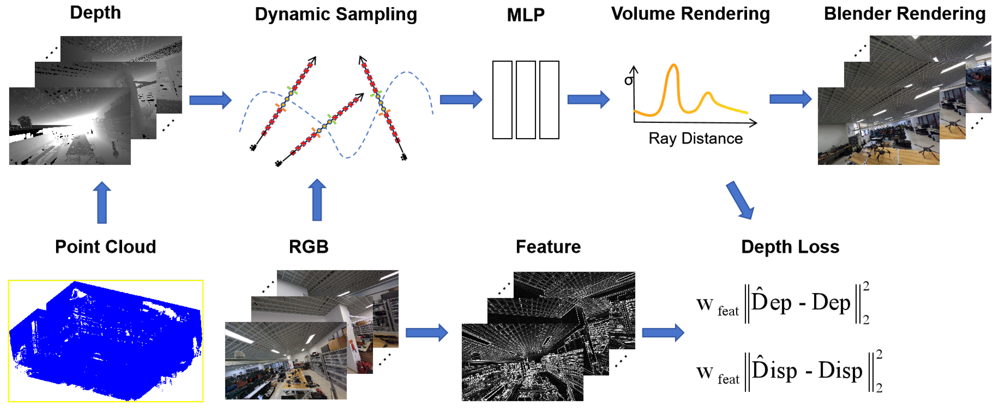
Figure 1 shows the general framework of our method. First, we input the point cloud and process it by projecting the point cloud to generate a depth map (
Section 3.1). Then, we input the image and use the depth information for dynamic sampling (
Section 3.3), which is then fed to the MLP for training. At the same time, we extract the corresponding feature maps from the image and weight the feature information with the depth loss (
Section 3.4). Finally, the image from the novel view is rendered. Our output image and depth map can be used to generate a high-quality point cloud (
Section 3.5).
3.1. Data Preprocessing
Considering the usability of the method in real life and the accuracy of the depth data, our method uses LiDAR data collected from a real scene. However, processing the collected point cloud into a depth map presents several challenges.
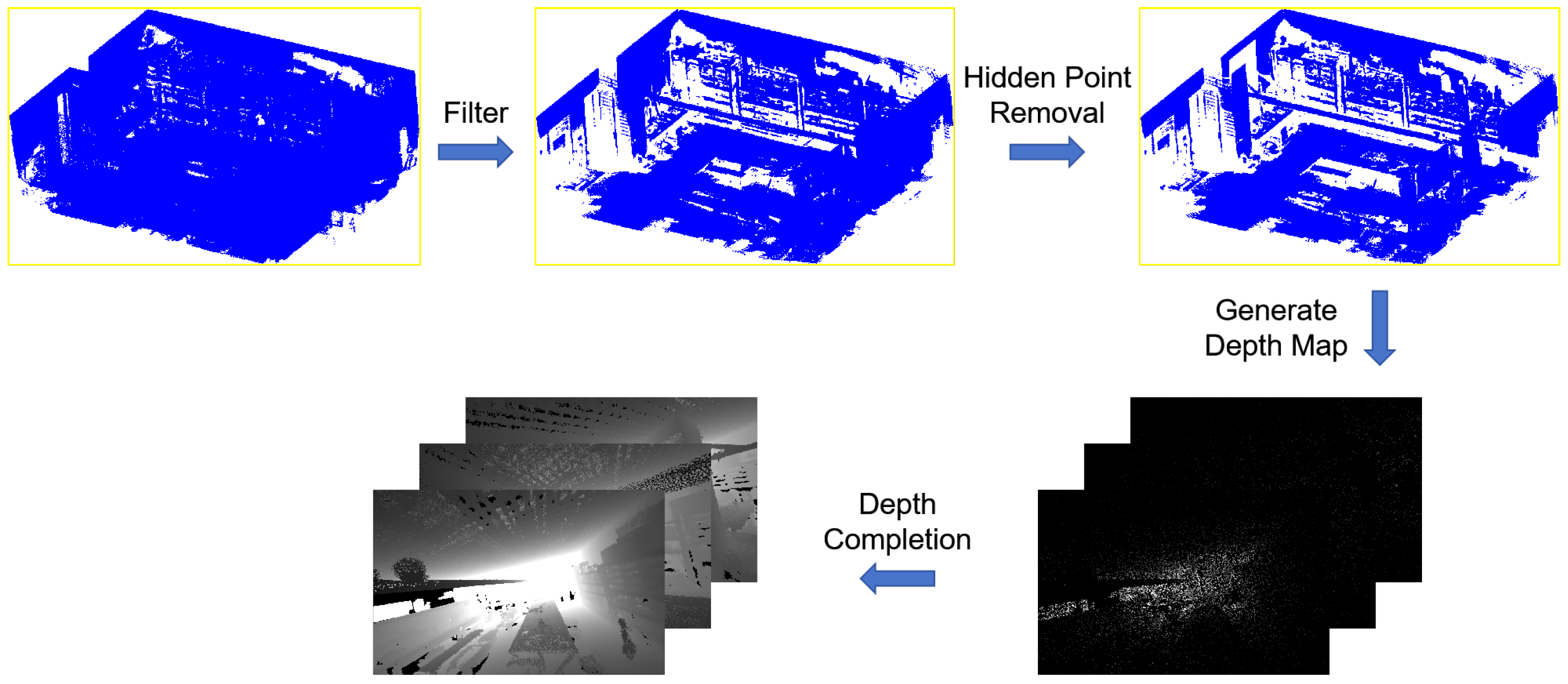
Figure 2 shows the complete data preprocessing flow.
Firstly, the acquired LiDAR point cloud often contains noise and voids. To address this issue, we apply a statistical outlier removal filter and low-pass filtering to eliminate floaters and sparse outliers. This processing effectively reduces error values in the generated depth map.
Secondly, generating depth maps by projecting point clouds directly from the camera position requires high accuracy of the camera position, but since the initial information obtained by the device during acquisition and processing may not always reflect the completely correct position, we refer to SfM’s method for adjusting the camera position to be more accurate, which effectively improves the quality of the depth maps as well as the results of our method.
However, when the point cloud is directly projected into a depth map, the resulting map exhibits perspective distortion, and it displays content from occluded areas that should not be visible. This is because, although the point cloud has a high point density, the points in the front cannot completely cover the points in the back when projected onto the image. Therefore, we remove the hidden points from the point cloud based on the corresponding camera position before projecting it into the depth map.
Finally, as the depth maps after the above processing are sparse and there are many places where the true depth values cannot be displayed, we have enhanced the depth completion method [
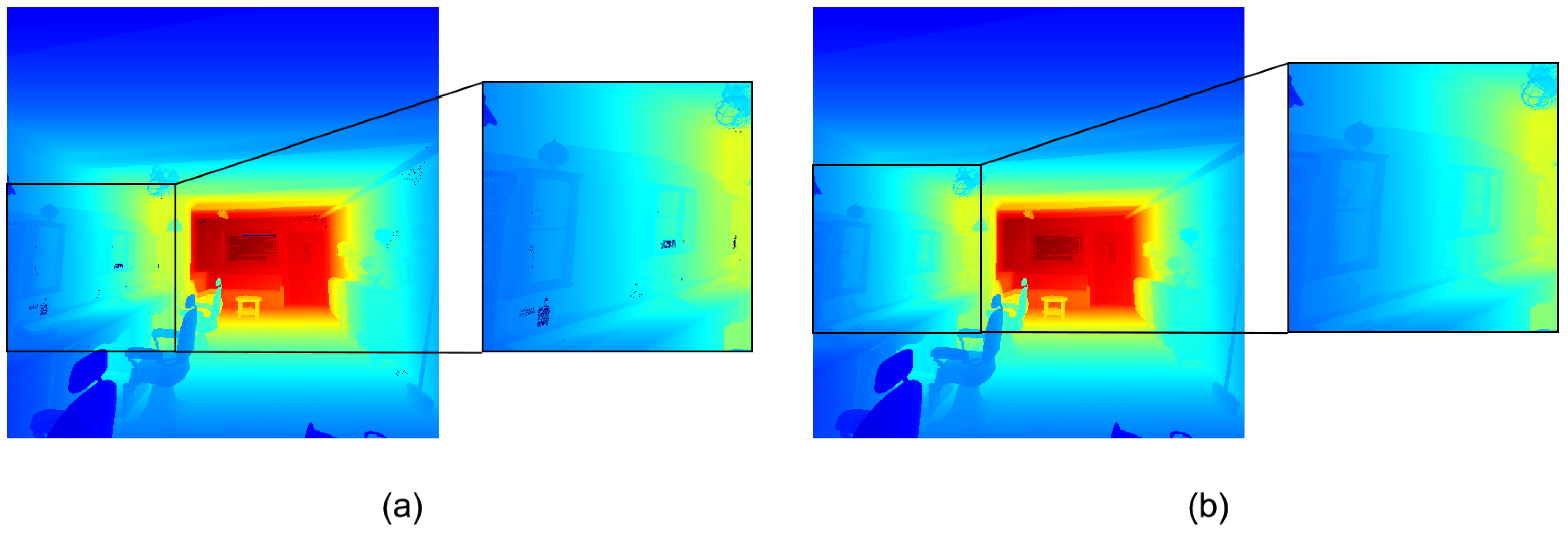
48] to fill in the missing values in the generated depth maps. It is worth noting that such processing can cause the depth map to become blurred at the edges, making it difficult to retain detail. Therefore, we made a small but critical change to the depth completion method so that it only changes the empty areas in the depth map that originally had a depth value of 0. This processing significantly improved the quality of our depth maps. A comparison of the visualisation before and after depth completion is shown in
Figure 3.
3.2. Depth Scale
Zip-NeRF proposes a new scale characterisation method to solve the spatial and depth jaggedness problems in the NeRF model so as to improve the quality of the rendered images. However, numerous experiments have shown that the predicted scales in unbounded scenes are inconsistent with the scales of real scenes. This inconsistency prevents the final generated depth maps from accurately representing the true depth values. As a result, the predicted depth map cannot be used to generate a point cloud with a uniform scale, nor can the input depth values be used to improve the method.
Therefore, we propose the concept of a depth scale. A separate optimiser is designed for the depth scale and its initial value is set to 1. During the training process, the depth scale multiplies the predicted depth values. The input depth map has uniform true-scale depth values, so with the depth loss proposed in
Section 3.4, the predicted depth values after multiplying the depth scale can converge to the depth values of the input depth map. Meanwhile, the depth scale can be fixed to a specific value to ensure a consistent scale between the depth values of the input depth map and the predicted depth values after multiplying the depth scale. The optimisation of the depth scale is then halted and used in the dynamic sampling presented in
Section 3.3. This is a simple yet effective process that guarantees that the depth values generated by the final prediction are consistent with the depth values of the real scene.
3.3. Dynamic Sampling
The original NeRF was sampled coarsely between fixed near and far planes to maximise the coverage of sampling points on each ray. However, the majority of the scene space does not correspond to any object surface, and the sampling points in these regions have volume density values predicted by the network that are close to zero, resulting in no contribution to the final results. Furthermore, a significant proportion of the scene is occupied by invalid sampling points, which hinders efficient resource utilisation.
Additionally, there is a sample imbalance between the limited number of valid sampling points located near the object’s surface and the numerous invalid sampling points that are not in the vicinity of the object’s surface. This imbalance may impede the network model’s quick convergence.
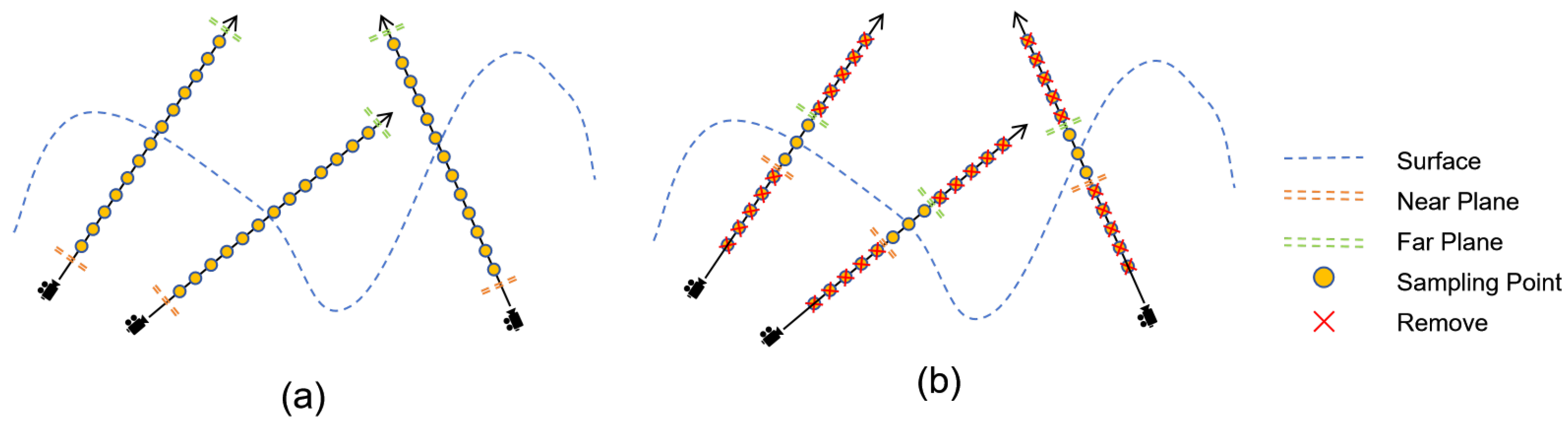
The dynamic sampling method enables effective use of the depth prior in order to limit the sampling range to near the depth value. This allows for the concentration of sampling points near the most likely surface of the object, ensuring rendering quality while reducing the number of invalid sampling points. Consequently, the convergence of the network model is sped up, and the airborne floaters problem in the rendered scene is alleviated. It also improves the quality of the predicted image and depth maps.
Figure 4 illustrates how the method adjusts the near and far planes of each ray based on the depth prior. This ensures that each ray is sampled only in the vicinity of the corresponding depth prior. The equations for the near and far planes are
where
ep is the depth value of the input depth image and
is a settable sampling range constraint, which was set to 1 in all experiments.
We use the spatial anti-aliasing proposed by the Zip-NeRF method; cones are used for sampling instead of rays. The addition of the dynamic sampling method significantly reduces the probability of invalid sampling and speeds up the convergence of the network model. This is a key factor in our method, achieving excellent results in a short time.
Figure 5 shows that the dynamic sampling method is very effective.
However, based on extensive experiments, it has been shown that using input depth information to constrain the sampling interval from the beginning can lead to errors in finding the correct depth within the interval. This is due to the difference in scale between the Zip-NeRF method and the real scene. Thus, we adopted the strategy of harmonising the two scales by using the parameter depth scale proposed in
Section 3.2 before implementing dynamic sampling. We stopped its change after a certain number of steps, and the depth information was then introduced to restrict the sampling interval, which is a straightforward and effective approach.
3.4. Loss Function
In recent years, many NeRF methods have included depth loss in their loss function. However, it is important to note that regions with significant variations in the image often have corresponding depth values in the real scene that are difficult to measure. Thus, prior to computing the depth loss, we extracted the feature map from the image and weighted the depth loss based on the feature values. We relied more on the colour information of the image in strong texture regions and more on the depth information in weak texture regions.
We use
as the feature weight, which is calculated by extracting feature values from the image:
where
, which is obtained by taking the cube root of the extracted feature values from the image. This adjustment amplifies the impact of the features on the depth loss.
Additionally, we observed that using only pure depth loss may be too simplistic, and therefore we introduced parallax loss. This is because depth loss is more likely to represent global depth and focuses on overall representation ability, while parallax directly reflects the distance between pixels, helping the network to better learn the details and structure of local regions. As our dynamic sampling method already effectively guides the network for depth prediction, we have designed the depth loss as a simple mean-squared loss:
The parameter balanced our depth loss with parallax loss, and in all experiments we set . is the depth value of the input depth image, is the parallax value obtained from , where . and represent calculated depth and parallax values.
With the above treatment, our total loss function is
where
denotes other losses in the Zip-NeRF method,
denotes the depth loss, and
is the hyperparameter used to balance the supervision of depth and colour.
It is important to note that depth information may not always be completely reliable due to limitations and issues in the acquisition and processing processes. Therefore, we limit the use of depth information to regions with depth values greater than 0.
3.5. Point Cloud Generation
Most novel view synthesis algorithms are limited to synthesising new perspective images and rendering videos of the scenes. The method presented in this study generates a dense and precise point cloud using a rendered high-quality image of a new viewpoint and a depth map. While other methods, such as Colmap, also generate point clouds, our method produces a denser point cloud with better precision and accuracy after filtering. This is demonstrated in
Figure 6.
The proposed depth scale in
Section 3.2 ensures consistency between the depth value in the rendered depth map and the scale of the real scene. This allows the point cloud generated by our method to be unified with the scale and position of the real scene’s point cloud, enabling it to be directly used for further work such as sparse point cloud complementation and model generation.
4. Results
4.1. Experimental Setup
The model used in this study is based on the Zip-NeRF method, with the addition of a proposed depth loss to the loss function. The overall model architecture is essentially identical to the Zip-NeRF method, with some additional modifications that we describe in
Section 3 and here.
In the experiments, two rounds of proposal sampling with 64 samples in each round are used, followed by 32 samples in the final NeRF sampling round. We have experimentally demonstrated that using such a number of samples can improve the speed of sampling while ensuring the quality of rendering. By using depth information to constrain the sampling interval, we can appropriately reduce the number of samples to improve the efficiency of our method. MipNeRF360 and ZipNeRF also employ this type of sampling. It is worth noting that a smaller number of samples is acceptable if the depth information used is reliable. Our proposal sampling rounds were both subject to our anti-aliased interlaminar loss. The first round had a rectangular pulse width of r = 0.03, while the second round had a pulse width of r = 0.003. Additionally, we used a loss multiplier of 0.01 in both rounds. In the comparison experiments, we uniformly used 32 samples for both coarse and fine sampling.
We add the weight of the depth scale when predicting the depth, which solves the problem that the obtained depth value is not consistent with the scale of the real scene in a simple way, and we induce the depth prediction with the input trustworthy depth information by dynamic sampling and by adding the depth loss in the loss function.
Considering the uniqueness of the depth scale and the special requirements for the variation in its values, we do not use the same learning rate that decays with the step size as for the other parameters but use a separate optimiser for the iterations. Its learning rate is set to 0.01 for the first 5000 training sessions; we set its learning rate to 0.001 when the step size is between 5000 and 10,000, and we stop its optimisation when it exceeds 10,000 sessions.
All experiments were conducted on a single NVIDIA GeForce RTX 2080 Ti GPU.
4.2. Dataset
Since our method needs to include depth data, we verified the validity of our method using a dataset collected by DoNeRF, which has very good quality, extremely fine textures, high frequency detail, and a large depth range for our experiments. The dataset was rendered using Blender, with bit poses randomly sampled in the view cell. Each scene in the original dataset consists of 300 high-quality images and depth maps.
To validate the effectiveness of our method under sparse viewpoint inputs, we purposely used only 11 images selected from the original training set as the new training set and 20 images as the new test set. For our comparison experiments, we primarily utilised two scenarios: a classroom and a hairdresser’s shop.
However, to ensure the validity of our results, we also collected data from real-life environments using LIDAR and cameras. This dataset is of exceptional quality, with a rich texture and a variety of challenging conditions, including occlusion, light and shadow changes, and specular reflections. It provides an accurate representation of the complex scenes found in real-world environments.
Our real scene is large and contains a large number of objects. Therefore, 96 high-quality images are used for our real dataset, of which 86 are used as the training set and 10 as the test set. Depth maps are generated by data preprocessing as described in
Section 3.1.
4.3. Evaluation Metrics
Peak Signal-to-Noise Ratio (PSNR) is a widely used metric for the objective assessment of images, based on a calculation of the error between corresponding pixels.
Structural Similarity (SSIM) [
49] is an evaluation metric used to measure the similarity of two images, which models distortion as a combination of brightness, contrast, and structure.
Learning Perceptual Image Block Similarity (LPIPS) [
50] is a metric for assessing image similarity based on deep learning. It compares deep features extracted by a neural network.
The time required to train each method is described in hours.
4.4. Comparison
Table 1 compares the prediction results of our method and other advanced methods. Our method was compared with NeRF, DoNeRF, and Zip-NeRF in the experiments, and our method had a clear advantage in all metrics. To show the advantage of our method in terms of the training time required, in addition to the 200,000 training epochs used by each method, we also compared our method with only 10,000 and 50,000 training epochs, and the experimental results proved that by using only forty minutes of time, our method can produce a very excellent result that can be compared with other advanced methods, which effectively mitigates the problem of the long training time required for NeRF.
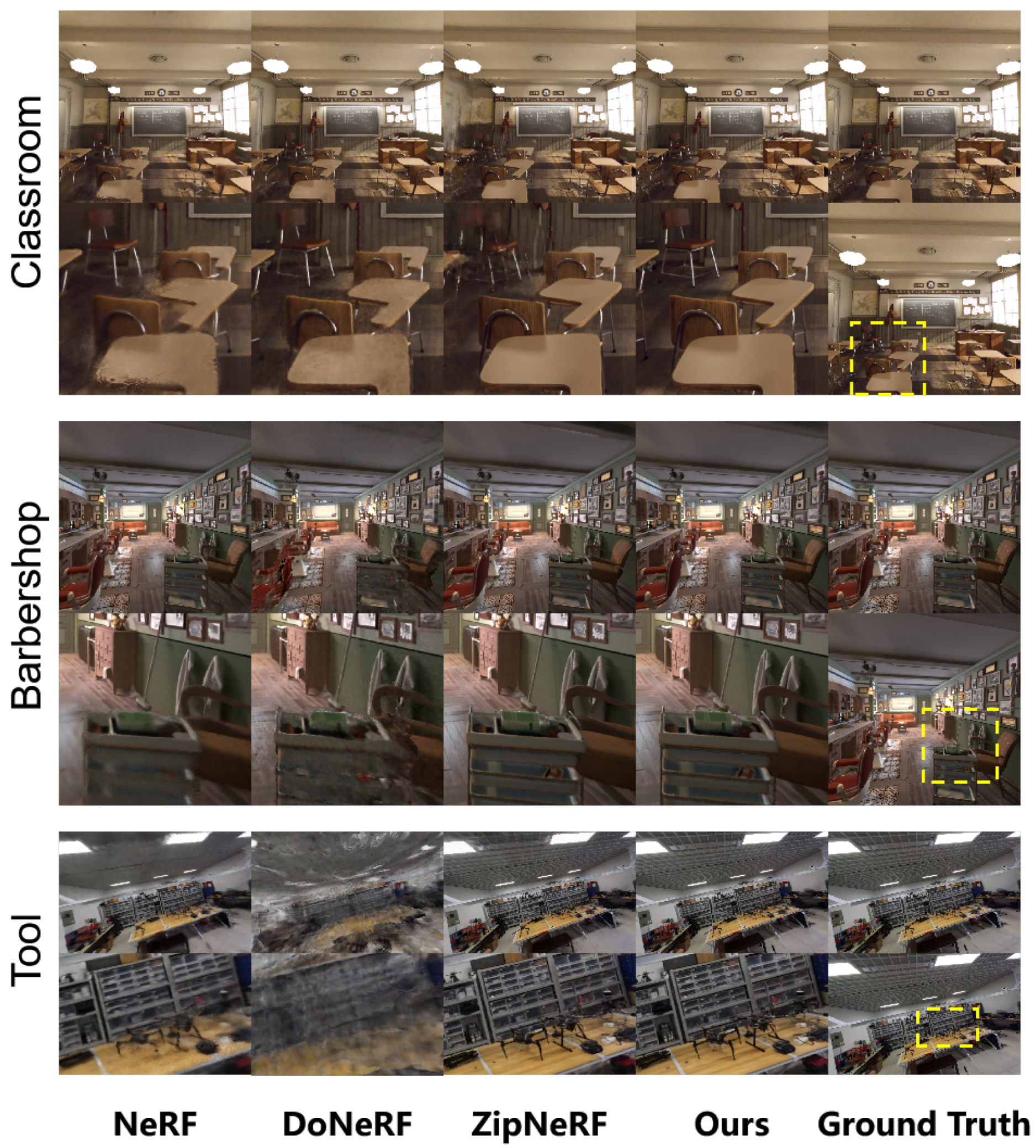
Figure 7 shows the rendering results of our method compared to other advanced methods. Each scene comprises a panorama and a local view for comparison purposes. Our method demonstrates excellent results for both panoramic and local views. The original NeRF does not incorporate an additional prior to guide model training or prediction, resulting in the significant blurring of newly rendered views using sparse sample points. DoNeRF uses depth information to train the sampling Oracle network, which assists the model in identifying optimal sampling locations. However, when the number of input images decreases, the prediction accuracy of the sampling Oracle network also decreases, resulting in a blurred new view. Although Zip-NeRF shows good results, it lacks depth information constraints, leading to missing and blurred details. Our method introduces a depth prior in the sampling method and the loss function to effectively guide the model to render high-quality images despite the reduced input images. It should be noted that DoNeRF exhibits poor performance on real scene datasets due to its heavy reliance on accurate depth information, whereas our approach can produce good results without requiring high-quality depth information.
4.5. Ablation Study
Experiments were conducted on relevant datasets to verify the effectiveness of dynamic sampling, depth loss, and feature weighting.
Table 2 shows that while the method using only some of these techniques does work, the hybrid approach is the most effective in all metrics, including SSIM, PSNR, and LPIPS.
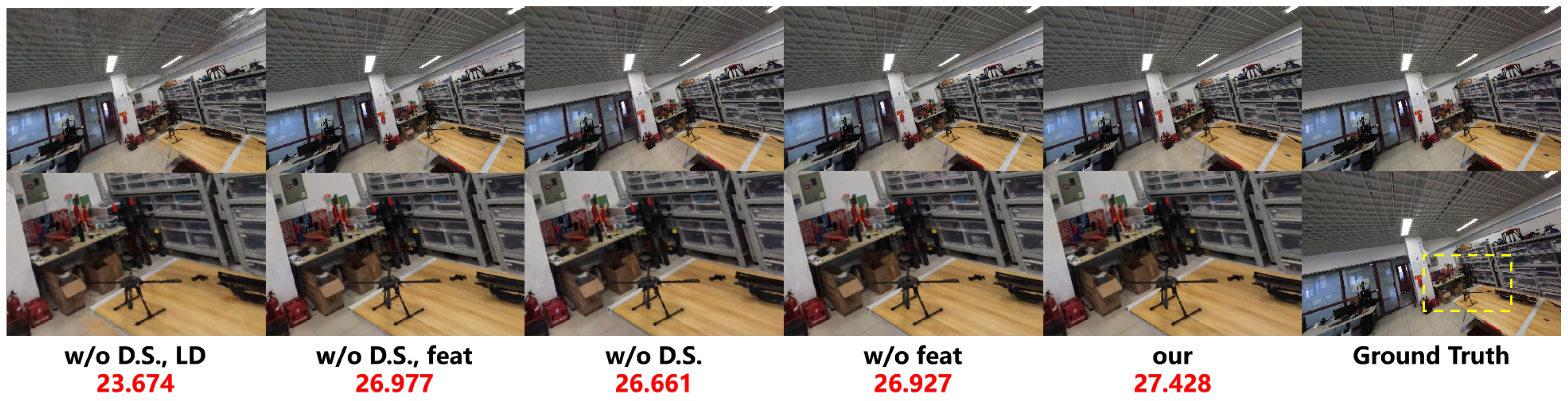
The ablation study clearly shows that the omission of dynamic sampling and depth loss leads to significant blurring and ghosting. Additionally, the lack of dynamic sampling methods results in a large number of invalid samples, which significantly impacts convergence speed and hinders the generation of high-quality rendered images within a short period. And, the absence of depth loss causes a focus solely on image information, disregarding depth information that could serve as a constraint. Furthermore, utilising a simple depth loss function without incorporating feature weights can result in indistinct occlusions near occluded objects and loss of detail due to the overbearing influence of depth information. As a result, it is imperative to differentiate the reliability of depth information in various regions by incorporating feature weights. Additionally, neglecting dynamic sampling methods increases the distance between sampling points and affects the convergence of the model. This can also make it difficult to accurately estimate the surface location of objects, resulting in blurred rendered images and the appearance of airborne floaters in the scene. If feature weights weighted according to depth loss are not used, some details may become blurred due to a possible lack of accurate depth information. Additionally, smoothed regions that should be more dependent on depth information may have uneven colours due to the excessive influence of the image.
Figure 8 shows the experimental results of the ablation study on a real scene dataset. The results demonstrate the effectiveness of dynamic sampling, depth loss, and feature weights in both the overall and detail parts. Notably, the use of dynamic sampling prevents significant blurring in the details.
5. Discussion
Our method outperforms the baselines in both qualitative and quantitative comparisons. In the sparse view condition, our method shows significant advantages on several public datasets, as well as the real datasets we created. The evaluation metrics demonstrate a significant improvement in the time it takes to compare the results of a 40-min training session to the results of a several-hour training session with baselines.
The NeRF method does not incorporate any additional a priori information to guide model training or prediction. This lack of guidance leads to inefficiency and poor results, particularly in sparse perspectives. In contrast, DoNeRF utilises depth information to train the sampling Oracle network. This approach helps the model to determine the optimal sampling location. However, the depth prediction network utilises only a single depth value as a training target, which may cause issues with transparent objects and specular surfaces. Additionally, it heavily relies on depth information, resulting in poor outcomes if the depth information is inaccurate. Although ZipNeRF shows better results, it lacks the constraints of depth information. This makes it unable to fully fit the surface and more susceptible to changes in illumination. Additionally, it uses a sampling method that increases the computational cost, making it difficult to train in a short period of time to achieve good results. In contrast, our method utilises depth-informed constrained sampling, which greatly improves efficiency while addressing the interference of transparent objects and specular surfaces, producing excellent results quickly and enabling the generation of high-quality dense point clouds.
Although our method is more efficient and produces higher-quality images than baselines, it still heavily relies on accurate depth information. Low-quality depth information may lead to incorrect sampling and failure to achieve the desired results, although we reduce the trustworthiness of the error depth by feature weights.
Additionally, our method is currently limited to static scenes, but we plan to extend its application to dynamic scenes in the future. To accomplish this objective, it is essential to consider dynamic NeRF techniques that integrate depth and spatio-temporal information for the reconstruction of lifelike 3D environments.
6. Conclusions
We present Dip-NeRF, which incorporates previous advances in three areas: scale-aware anti-aliasing NeRF, fast grid-based NeRF training, and NeRF incorporating depth. The method utilises fast dynamic sampling with depth information and constraints to achieve lower error rates than previous techniques, allowing for less time to be spent on training. The experimental results demonstrate that the method is effective in reducing training time and generating high-quality new-view images and dense point clouds using a small number of images, even in complex scenes with a large number of occlusions. Although our method enables the rapid synthesis of high-quality new perspective images and point cloud models using a small number of input images, it relies on depth a priori information. Therefore, the quality of the synthesised images may degrade if the depth maps are of poor quality or if the depth a priori information is incorrect. Depth inaccuracies can arise due to transparent objects, occlusions, and light reflections in real scenes, which can affect the quality of the input depth map. Our method is robust to such inaccuracies, but they can still lead to a decrease in prediction accuracy. Future work should evaluate the credibility of the depth information before using it. Additionally, a larger sampling range and smaller depth loss weights should be applied to the depth-unreliable regions to further improve the model’s robustness in cases of unreliable depth a priori information. Additionally, our method demonstrates outstanding performance in static scenes, even in real-world scenarios with numerous occlusions and intricate lighting conditions. However, it may not perform as well in dynamic scenes with significant variations. Acquiring data in real-world settings is challenging due to the need to ensure scene stability and account for changes in lighting, moving objects, and other factors. Based on our current method, we can combine spatio-temporal information to reconstruct dynamic 3D scenes and point cloud models more accurately. This will provide better technical support for future work.
Author Contributions
Conceptualisation, S.Q. and J.X.; methodology, S.Q. and J.X.; software, S.Q.; validation, S.Q.; formal analysis, J.G. and S.Q.; investigation, J.X. and J.G.; resources, S.Q., J.X. and J.G.; data curation, S.Q.; writing—original draft preparation, S.Q.; writing—review and editing, J.G., S.Q. and J.X.; visualisation, S.Q.; supervision, J.X. and J.G.; project administration, J.X. and J.G.; funding acquisition, J.X. and J.G. All authors have read and agreed to the published version of the manuscript.
Funding
This work was supported in part by the Ningbo Science and Technology Innovation 2025 Major Project (grant: 2021Z037).
Data Availability Statement
The data that support the findings of this study are available from the author S.Q. upon reasonable request.
Acknowledgments
We would like to thank the editors and the anonymous reviewers for their insightful comments and constructive suggestions.
Conflicts of Interest
The authors declare no conflicts of interest.
References
- Mildenhall, B.; Srinivasan, P.P.; Tancik, M.; Barron, J.T.; Ramamoorthi, R.; Ng, R. Nerf: Representing scenes as neural radiance fields for view synthesis. Commun. ACM 2021, 65, 99–106. [Google Scholar] [CrossRef]
- Schonberger, J.L.; Frahm, J.M. Structure-from-motion revisited. In Proceedings of the IEEE Conference on Computer Vision and Pattern Recognition, Las Vegas, NV, USA, 27–30 June 2016; pp. 4104–4113. [Google Scholar]
- Thies, J.; Zollhöfer, M.; Nießner, M. Deferred neural rendering: Image synthesis using neural textures. ACM Trans. Graph. (TOG) 2019, 38, 1–12. [Google Scholar] [CrossRef]
- Liu, L.; Xu, W.; Zollhoefer, M.; Kim, H.; Bernard, F.; Habermann, M.; Wang, W.; Theobalt, C. Neural rendering and reenactment of human actor videos. ACM Trans. Graph. (TOG) 2019, 38, 1–14. [Google Scholar] [CrossRef]
- Liu, L.; Xu, W.; Habermann, M.; Zollhöfer, M.; Bernard, F.; Kim, H.; Wang, W.; Theobalt, C. Neural human video rendering by learning dynamic textures and rendering-to-video translation. arXiv 2020, arXiv:2001.04947. [Google Scholar]
- Habermann, M.; Liu, L.; Xu, W.; Zollhoefer, M.; Pons-Moll, G.; Theobalt, C. Real-time deep dynamic characters. ACM Trans. Graph. (ToG) 2021, 40, 1–16. [Google Scholar] [CrossRef]
- Lombardi, S.; Simon, T.; Saragih, J.; Schwartz, G.; Lehrmann, A.; Sheikh, Y. Neural volumes: Learning dynamic renderable volumes from images. arXiv 2019, arXiv:1906.07751. [Google Scholar] [CrossRef]
- Sitzmann, V.; Thies, J.; Heide, F.; Nießner, M.; Wetzstein, G.; Zollhofer, M. Deepvoxels: Learning persistent 3D feature embeddings. In Proceedings of the IEEE/CVF Conference on Computer Vision and Pattern Recognition, Long Beach, CA, USA, 15–20 June 2019; pp. 2437–2446. [Google Scholar]
- Aliev, K.A.; Sevastopolsky, A.; Kolos, M.; Ulyanov, D.; Lempitsky, V. Neural point-based graphics. In Computer Vision—ECCV 2020: 16th European Conference, Glasgow, UK, 23–28 August 2020, Proceedings, Part XXII; Springer: Cham, Switzerland, 2020; pp. 696–712. [Google Scholar]
- Wu, M.; Wang, Y.; Hu, Q.; Yu, J. Multi-view neural human rendering. In Proceedings of the IEEE/CVF Conference on Computer Vision and Pattern Recognition, Seattle, WA, USA, 14–19 June 2020; pp. 1682–1691. [Google Scholar]
- Kopanas, G.; Philip, J.; Leimkühler, T.; Drettakis, G. Point-Based Neural Rendering with Per-View Optimization. In Computer Graphics Forum; Wiley Online Library: Hoboken, NJ, USA, 2021; Volume 40, pp. 29–43. [Google Scholar]
- Rückert, D.; Franke, L.; Stamminger, M. Adop: Approximate differentiable one-pixel point rendering. ACM Trans. Graph. (ToG) 2022, 41, 1–14. [Google Scholar] [CrossRef]
- Debevec, P.; Taylor, C.J.; Malik, J. Modeling and Rendering Architecture from Photographs: A Hybrid Geometry-and Image-Based Approach. In Proceedings of the 23rd International Conference on Computer Graphics and Interactive Techniques, New Orleans, LA, USA, 4–9 August 1996; pp. 11–20. [Google Scholar]
- Sinha, S.; Steedly, D.; Szeliski, R. Piecewise planar stereo for image-based rendering. In Proceedings of the 2009 International Conference on Computer Vision, Kyoto, Japan, 29 September–2 October 2009; pp. 1881–1888. [Google Scholar]
- Chaurasia, G.; Sorkine, O.; Drettakis, G. Silhouette-Aware Warping for Image-Based Rendering. In Computer Graphics Forum; Wiley Online Library: Hoboken, NJ, USA, 2011; Volume 30, pp. 1223–1232. [Google Scholar]
- Chaurasia, G.; Duchene, S.; Sorkine-Hornung, O.; Drettakis, G. Depth synthesis and local warps for plausible image-based navigation. ACM Trans. Graph. (TOG) 2013, 32, 1–12. [Google Scholar] [CrossRef]
- De Bonet, J.S.; Viola, P. Poxels: Probabilistic voxelized volume reconstruction. In Proceedings of the International Conference on Computer Vision (ICCV), Corfu, Greece, 20–25 September 1999; Volume 2, p. 2. [Google Scholar]
- Kutulakos, K.N.; Seitz, S.M. A theory of shape by space carving. Int. J. Comput. Vis. 2000, 38, 199–218. [Google Scholar] [CrossRef]
- Kolmogorov, V.; Zabih, R. Multi-camera scene reconstruction via graph cuts. In Computer Vision—ECCV 2002: 7th European Conference on Computer Vision, Copenhagen, Denmark, 28–31 May 2002, Proceedings, Part III; Springer: Berlin/Heidelberg, Germany, 2002; pp. 82–96. [Google Scholar]
- Esteban, C.H.; Schmitt, F. Silhouette and stereo fusion for 3D object modeling. Comput. Vis. Image Underst. 2004, 96, 367–392. [Google Scholar] [CrossRef]
- Seitz, S.M.; Curless, B.; Diebel, J.; Scharstein, D.; Szeliski, R. A comparison and evaluation of multi-view stereo reconstruction algorithms. In Proceedings of the 2006 IEEE Computer Society Conference on Computer Vision and Pattern Recognition (CVPR’06), New York, NY, USA, 17–22 June 2006; Volume 1, pp. 519–528. [Google Scholar]
- Furukawa, Y.; Ponce, J. Accurate, dense, and robust multiview stereopsis. IEEE Trans. Pattern Anal. Mach. Intell. 2009, 32, 1362–1376. [Google Scholar] [CrossRef] [PubMed]
- Schönberger, J.L.; Zheng, E.; Frahm, J.M.; Pollefeys, M. Pixelwise view selection for unstructured multi-view stereo. In Computer Vision—ECCV 2016: 14th European Conference, Amsterdam, The Netherlands, 11–14 October 2016, Proceedings, Part III; Springer: Cham, Switzerland, 2016; pp. 501–518. [Google Scholar]
- Chen, A.; Xu, Z.; Zhao, F.; Zhang, X.; Xiang, F.; Yu, J.; Su, H. Mvsnerf: Fast generalizable radiance field reconstruction from multi-view stereo. In Proceedings of the IEEE/CVF International Conference on Computer Vision, Virtual, 11–17 October 2021; pp. 14124–14133. [Google Scholar]
- Wang, Q.; Wang, Z.; Genova, K.; Srinivasan, P.P.; Zhou, H.; Barron, J.T.; Martin-Brualla, R.; Snavely, N.; Funkhouser, T. Ibrnet: Learning multi-view image-based rendering. In Proceedings of the IEEE/CVF Conference on Computer Vision and Pattern Recognition, Virtual, 19–25 June 2021; pp. 4690–4699. [Google Scholar]
- Yu, A.; Ye, V.; Tancik, M.; Kanazawa, A. pixelnerf: Neural radiance fields from one or few images. In Proceedings of the IEEE/CVF Conference on Computer Vision and Pattern Recognition, Virtual, 19–25 June 2021; pp. 4578–4587. [Google Scholar]
- Deng, K.; Liu, A.; Zhu, J.Y.; Ramanan, D. Depth-supervised nerf: Fewer views and faster training for free. In Proceedings of the IEEE/CVF Conference on Computer Vision and Pattern Recognition, New Orleans, LA, USA, 18–24 June 2022; pp. 12882–12891. [Google Scholar]
- Roessle, B.; Barron, J.T.; Mildenhall, B.; Srinivasan, P.P.; Nießner, M. Dense depth priors for neural radiance fields from sparse input views. In Proceedings of the IEEE/CVF Conference on Computer Vision and Pattern Recognition, New Orleans, LA, USA, 18–24 June 2022; pp. 12892–12901. [Google Scholar]
- Curless, B.; Levoy, M. A volumetric method for building complex models from range images. In Proceedings of the 23rd Annual Conference on Computer Graphics and Interactive Techniques, New Orleans, LA, USA, 4–9 August 1996; pp. 303–312. [Google Scholar]
- Izadi, S.; Kim, D.; Hilliges, O.; Molyneaux, D.; Newcombe, R.; Kohli, P.; Shotton, J.; Hodges, S.; Freeman, D.; Davison, A.; et al. Kinectfusion: Real-time 3D reconstruction and interaction using a moving depth camera. In Proceedings of the 24th Annual ACM Symposium on User Interface Software and Technology, Santa Barbara, CA, USA, 16–19 October 2011; pp. 559–568. [Google Scholar]
- Nießner, M.; Zollhöfer, M.; Izadi, S.; Stamminger, M. Real-time 3D reconstruction at scale using voxel hashing. ACM Trans. Graph. (ToG) 2013, 32, 1–11. [Google Scholar] [CrossRef]
- Dai, A.; Nießner, M.; Zollhöfer, M.; Izadi, S.; Theobalt, C. Bundlefusion: Real-time globally consistent 3D reconstruction using on-the-fly surface reintegration. ACM Trans. Graph. (ToG) 2017, 36, 1. [Google Scholar] [CrossRef]
- Murez, Z.; Van As, T.; Bartolozzi, J.; Sinha, A.; Badrinarayanan, V.; Rabinovich, A. Atlas: End-to-end 3D scene reconstruction from posed images. In Computer Vision—ECCV 2020: 16th European Conference, Glasgow, UK, 23–28 August 2020, Proceedings, Part VII; Springer: Cham, Switzerland, 2020; pp. 414–431. [Google Scholar]
- Pfister, H.; Zwicker, M.; Van Baar, J.; Gross, M. Surfels: Surface elements as rendering primitives. In Proceedings of the 27th Annual Conference on Computer Graphics and Interactive Techniques, New Orleans, LA, USA, 23–28 July 2000; pp. 335–342. [Google Scholar]
- Kazhdan, M.; Bolitho, M.; Hoppe, H. Poisson surface reconstruction. In Proceedings of the Fourth Eurographics Symposium on Geometry Processing, Cagliari, Sardinia, Italy, 26–28 June 2006; Volume 7, pp. 61–70. [Google Scholar]
- Marton, Z.C.; Rusu, R.B.; Beetz, M. On fast surface reconstruction methods for large and noisy point clouds. In Proceedings of the 2009 IEEE International Conference on Robotics and Automation, Kobe, Japan, 12–17 May 2009; pp. 3218–3223. [Google Scholar]
- Turki, H.; Ramanan, D.; Satyanarayanan, M. Mega-nerf: Scalable construction of large-scale nerfs for virtual fly-throughs. In Proceedings of the IEEE/CVF Conference on Computer Vision and Pattern Recognition, New Orleans, LA, USA, 18–24 June 2022; pp. 12922–12931. [Google Scholar]
- Tancik, M.; Casser, V.; Yan, X.; Pradhan, S.; Mildenhall, B.; Srinivasan, P.P.; Barron, J.T.; Kretzschmar, H. Block-nerf: Scalable large scene neural view synthesis. In Proceedings of the IEEE/CVF Conference on Computer Vision and Pattern Recognition, New Orleans, LA, USA, 18–24 June 2022; pp. 8248–8258. [Google Scholar]
- Zhang, K.; Riegler, G.; Snavely, N.; Koltun, V. Nerf++: Analyzing and improving neural radiance fields. arXiv 2020, arXiv:2010.07492. [Google Scholar]
- Barron, J.T.; Mildenhall, B.; Tancik, M.; Hedman, P.; Martin-Brualla, R.; Srinivasan, P.P. Mip-nerf: A multiscale representation for anti-aliasing neural radiance fields. In Proceedings of the IEEE/CVF International Conference on Computer Vision, Virtual, 11–17 October 2021; pp. 5855–5864. [Google Scholar]
- Barron, J.T.; Mildenhall, B.; Verbin, D.; Srinivasan, P.P.; Hedman, P. Mip-nerf 360: Unbounded anti-aliased neural radiance fields. In Proceedings of the IEEE/CVF Conference on Computer Vision and Pattern Recognition, New Orleans, LA, USA, 18–24 June 2022; pp. 5470–5479. [Google Scholar]
- Kerbl, B.; Kopanas, G.; Leimkuehler, T.; Drettakis, G. 3D Gaussian Splatting for Real-Time Radiance Field Rendering. ACM Trans. Graph. (TOG) 2023, 42, 1–14. [Google Scholar] [CrossRef]
- Lee, D.; Lee, K.M. Dense Depth-Guided Generalizable NeRF. IEEE Signal Process. Lett. 2023, 30, 75–79. [Google Scholar] [CrossRef]
- Neff, T.; Stadlbauer, P.; Parger, M.; Kurz, A.; Mueller, J.H.; Chaitanya, C.R.A.; Kaplanyan, A.; Steinberger, M. DONeRF: Towards Real-Time Rendering of Compact Neural Radiance Fields using Depth Oracle Networks. In Computer Graphics Forum; Wiley Online Library: Hoboken, NJ, USA, 2021; Volume 40, pp. 45–59. [Google Scholar]
- Wei, Y.; Liu, S.; Rao, Y.; Zhao, W.; Lu, J.; Zhou, J. Nerfingmvs: Guided optimization of neural radiance fields for indoor multi-view stereo. In Proceedings of the IEEE/CVF International Conference on Computer Vision, Virtual, 11–17 October 2021; pp. 5610–5619. [Google Scholar]
- Wang, G.; Chen, Z.; Loy, C.C.; Liu, Z. Sparsenerf: Distilling depth ranking for few-shot novel view synthesis. arXiv 2023, arXiv:2303.16196. [Google Scholar]
- Li, J.; Zhang, J.; Bai, X.; Zheng, J.; Ning, X.; Zhou, J.; Gu, L. DNGaussian: Optimizing Sparse-View 3D Gaussian Radiance Fields with Global-Local Depth Normalization. arXiv 2024, arXiv:2403.06912. [Google Scholar]
- Ku, J.; Harakeh, A.; Waslander, S.L. In defense of classical image processing: Fast depth completion on the cpu. In Proceedings of the 2018 15th Conference on Computer and Robot Vision (CRV), Toronto, ON, Canada, 9–11 May 2018; pp. 16–22. [Google Scholar]
- Wang, Z.; Bovik, A.C.; Sheikh, H.R.; Simoncelli, E.P. Image quality assessment: From error visibility to structural similarity. IEEE Trans. Image Process. 2004, 13, 600–612. [Google Scholar] [CrossRef]
- Zhang, R.; Isola, P.; Efros, A.A.; Shechtman, E.; Wang, O. The unreasonable effectiveness of deep features as a perceptual metric. In Proceedings of the IEEE Conference on Computer Vision and Pattern Recognition, Salt Lake City, UT, USA, 18–22 June 2018; pp. 586–595. [Google Scholar]
Figure 1.
This is the general framework of our method. The input data are images, corresponding camera poses, and a point cloud. First, we obtain the corresponding depth images by projecting the point cloud based on the camera poses, and then we use the depth information to constrain the sampling interval. We then use the images to generate feature maps, and use the features to weight the depth loss in order to render high-quality images of the new perspective. Note that our input point cloud is colourless and is therefore represented in blue for ease of display.
Figure 2.
The data preprocessing process consists of several steps. Firstly, the collected dense point cloud is filtered to remove any noise and moving objects. Next, we filter out any regions of the point cloud that are not visible due to occlusion in the current viewpoint using the hidden point removal method based on the camera position. Then, we project the point cloud to obtain the corresponding depth image. Finally, we improve the depth completion method and use it to obtain the final depth map. Note that our input point cloud is colourless and is therefore represented in blue for ease of display.
Figure 3.
To demonstrate the effectiveness of our improved depth completion method, we present a comparison of the visualisation of a depth map before (a) and after (b) the application of the method. The figure clearly illustrates that the method is highly effective in filling the gaps in the depth map, resulting in a significant improvement in its quality.
Figure 4.
(a) The original NeRF sampling method is used for wide range sampling without depth priors. (b) A dynamic sampling approach is employed, which removes several sampling points away from the object’s surface and only acquires sampling points near it.
Figure 4.
(a) The original NeRF sampling method is used for wide range sampling without depth priors. (b) A dynamic sampling approach is employed, which removes several sampling points away from the object’s surface and only acquires sampling points near it.
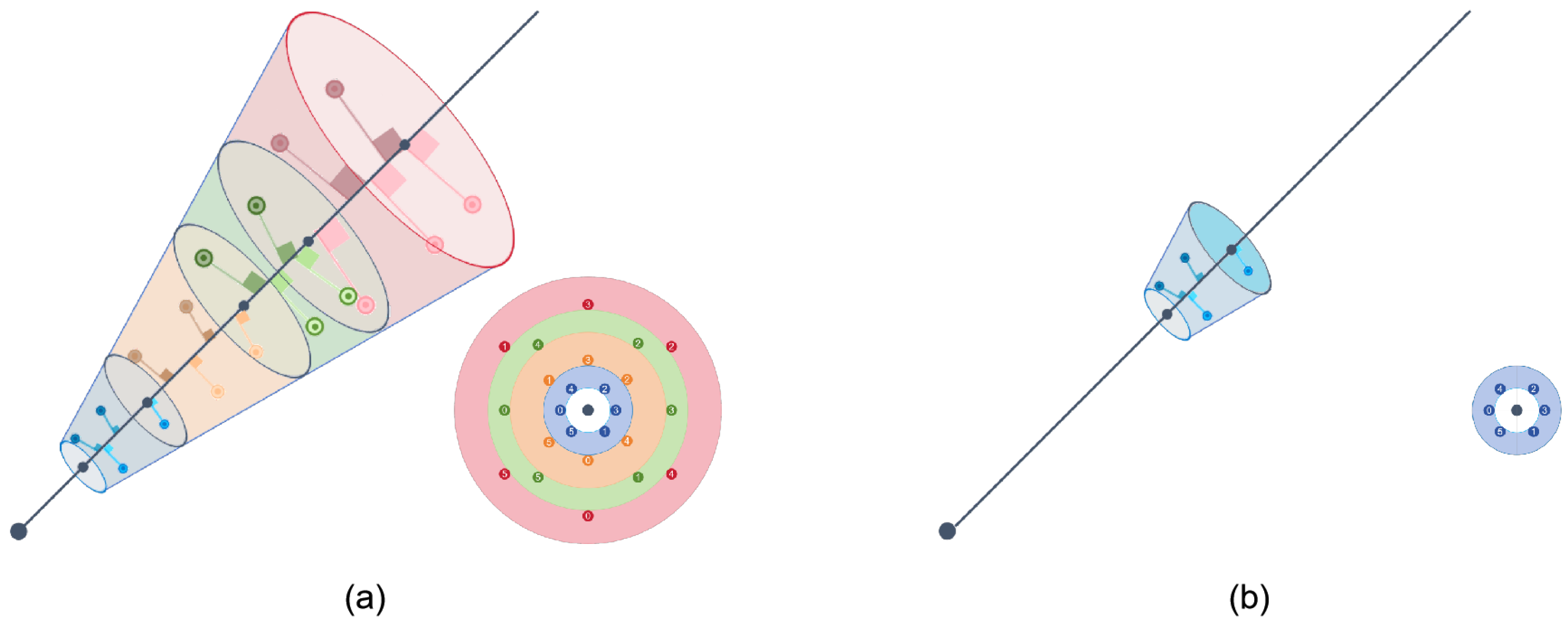
Figure 5.
Here we show a toy 3D ray with an exaggerated pixel width (viewed along the ray as an inset). (a) It is divided into 4 frustums denoted by colour. We multisample each frustum with a hexagonal pattern. (b) It is intercepted by the depth information and only a shorter part of it remains. We multisample this part with a hexagonal pattern.
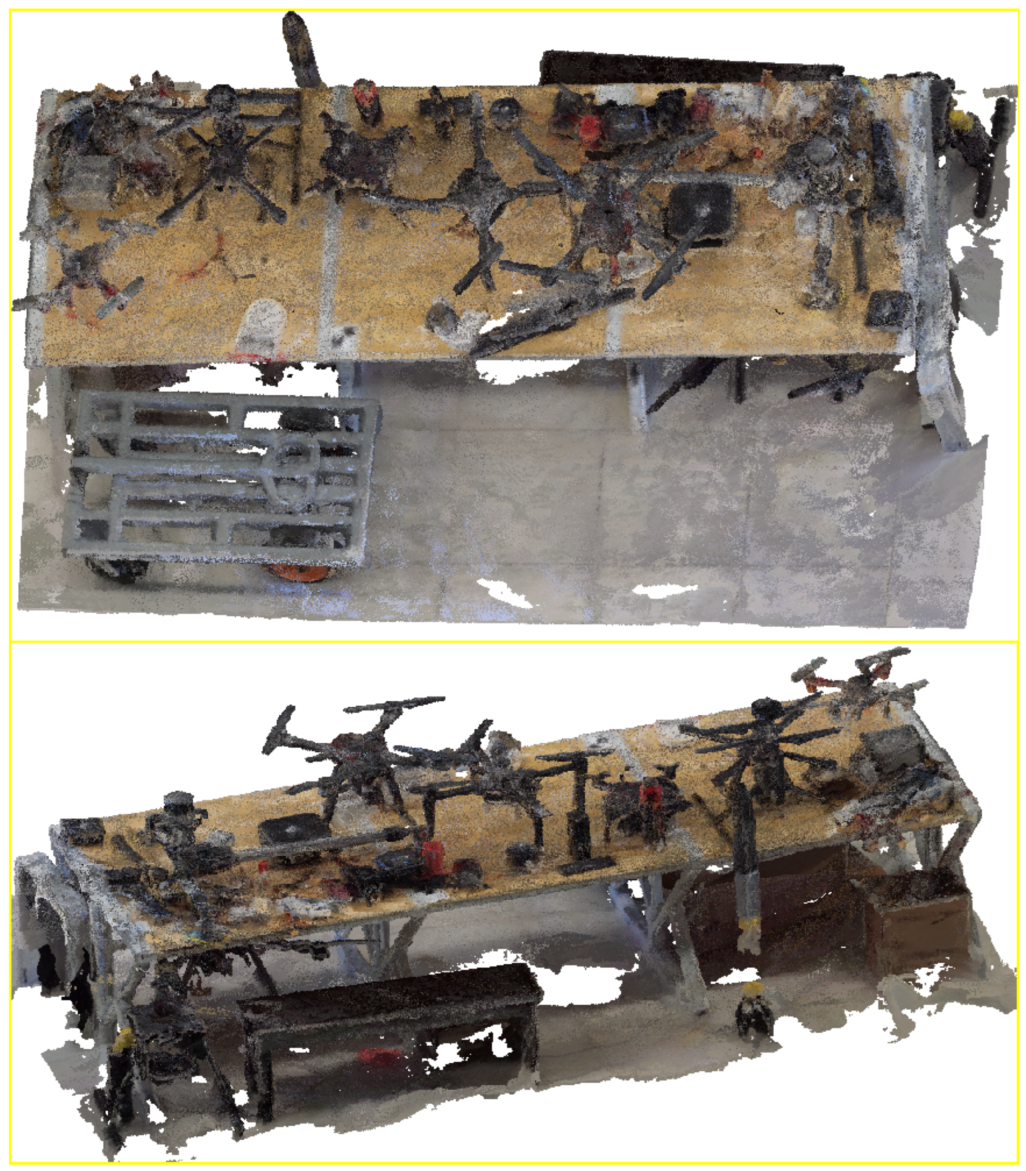
Figure 6.
High-quality point cloud generated using our methodology.
Figure 6.
High-quality point cloud generated using our methodology.
Figure 7.
Comparison of results between our method and other advanced methods. Each scene has a panorama and a partial view for comparison. Additionally, our method shows the best results for both panoramas and partial views.
Figure 7.
Comparison of results between our method and other advanced methods. Each scene has a panorama and a partial view for comparison. Additionally, our method shows the best results for both panoramas and partial views.
Figure 8.
Experimental results of the ablation study on the Tool real scenarios dataset. The results include a panoramic and a local view for comparison, with the PSNR values for each result highlighted in bold red.
Figure 8.
Experimental results of the ablation study on the Tool real scenarios dataset. The results include a panoramic and a local view for comparison, with the PSNR values for each result highlighted in bold red.
Table 1.
Quantitative comparison results for the three datasets, where the bold values are the best. The test results of different methods show that our method trained with only 40 min of time gives better results than the other methods. This shows that our method is more efficient. Additionally, when trained for the same number of epochs as the other methods, our method produces significantly better results than the baseline methods.
| | Classroom | Barbershop | Tool | Average |
|---|
|
Method
|
SSIM↑
|
PSNR↑
|
LPIPS↓
|
Time (h)↓
|
SSIM↑
|
PSNR↑
|
LPIPS↓
|
Time (h)↓
|
SSIM↑
|
PSNR↑
|
LPIPS↓
|
Time (h)↓
|
SSIM↑
|
PSNR↑
|
LPIPS↓
|
Time (h)↓
|
|---|
| NeRF | 0.945 | 28.135 | 0.159 | 5.73 | 0.894 | 25.768 | 0.186 | 5.68 | 0.698 | 22.059 | 0.425 | 5.07 | 0.846 | 25.321 | 0.257 | 5.49 |
| DoNeRF | 0.950 | 28.218 | 0.127 | 5.00 | 0.888 | 25.639 | 0.183 | 4.88 | 0.543 | 16.064 | 0.565 | 4.76 | 0.794 | 23.307 | 0.292 | 4.88 |
| Zip-NeRF | 0.960 | 28.121 | 0.084 | 13.36 | 0.940 | 28.536 | 0.085 | 13.58 | 0.817 | 24.731 | 0.160 | 13.25 | 0.906 | 27.129 | 0.110 | 13.40 |
| Ours (1w epochs) | 0.982 | 33.008 | 0.040 | 0.67 | 0.938 | 29.422 | 0.106 | 0.68 | 0.836 | 25.175 | 0.139 | 0.71 | 0.919 | 29.202 | 0.095 | 0.69 |
| Ours (5w epochs) | 0.984 | 33.540 | 0.032 | 3.33 | 0.946 | 29.978 | 0.084 | 3.42 | 0.863 | 26.290 | 0.097 | 3.40 | 0.931 | 29.936 | 0.071 | 3.38 |
| Ours | 0.985 | 34.125 | 0.031 | 13.33 | 0.949 | 30.169 | 0.073 | 13.67 | 0.881 | 27.574 | 0.068 | 13.20 | 0.938 | 30.623 | 0.057 | 13.40 |
Table 2.
Ablation studies performed on our model, where the bold values are the best. The table shows a quantitativite comparison of Dip-NeRF without dynamic sampling and depth loss (w/o D.S., ), without dynamic sampling and feature weighting (w/o D.S., feat), without dynamic sampling (w/o D.S.), and without feature weights (w/o feat).
| Method | SSIM↑ | PSNR↑ | LPIPS↓ |
|---|
| Ours (w/o D.S., ) | 0.817 | 24.731 | 0.160 |
| Ours (w/o D.S., feat) | 0.876 | 27.118 | 0.078 |
| Ours (w/o D.S.) | 0.868 | 26.795 | 0.084 |
| Ours (w/o feat) | 0.877 | 27.179 | 0.074 |
| Ours | 0.881 | 27.574 | 0.068 |
| Disclaimer/Publisher’s Note: The statements, opinions and data contained in all publications are solely those of the individual author(s) and contributor(s) and not of MDPI and/or the editor(s). MDPI and/or the editor(s) disclaim responsibility for any injury to people or property resulting from any ideas, methods, instructions or products referred to in the content. |
© 2024 by the authors. Licensee MDPI, Basel, Switzerland. This article is an open access article distributed under the terms and conditions of the Creative Commons Attribution (CC BY) license (https://creativecommons.org/licenses/by/4.0/).


