In this work, an automotive-grade INS is used. Therefore, the loosely-coupled filter with feedback is utilized. Loose GPS/INS integration occurs at the PVT (position, velocity and time) level. This means that the PVT measurements from the GPS are blended with the PVA (position, velocity and attitude) estimates of the INS. In the closed loop configuration, the inertial sensor errors estimated by the filter are fed back to the INS equations to compensate for the accelerometer and gyro errors. The most common fusing filter used for loosely-coupled GPS/INS is the extended Kalman filter (EKF) [
14] and is the filter of choice for this work. Refer to [
16,
17] for further specific details on the Kalman filter.
3.6.1. Navigation Error State EKF with Closed Loop Feedback
The system model for navigation states consists of the mechanization equations,
Equations (10)–
(12), which are nonlinear, and the models for the IMU biases. The linearized error state formulation of the mechanization equations was discussed as an item of interest of the standalone inertial navigation algorithm and formed
Equations (28)–
(30). While the INS states are error states, the remaining states are the full bias states of the accelerometer and gyro from the IMU. Accordingly for the cascaded navigation EKF, the error state vector is defined as:
Remember that the position vector
p is a vector of latitude, longitude and altitude,
vn is a velocity vector of north, east and down velocities and
ψnb is an attitude vector of roll, pitch and yaw. Note that the position states are not necessarily required to estimate the attitude, but are included in the formulation, because the typical user is also interested in the position information. The two bias vectors are included to account for the biases present in the IMU, where
is comprised of the three bias states corresponding to the accelerometer biases, and similarly,
is comprised of the gyro biases.
The IMU model consists of random noise and a bias added to the accelerations and angular velocities. The biases are modeled as a random walk. Specifically, the bias models for a low-cost inertial IMU are:
Note that the biases are a function of time, with some components that are modeled as stochastic processes. Both the accelerometer biases and the gyro biases are the sum of three random processes. The terms
and
represent the constant null shifts of the accelerometer and gyro. They are essentially static biases that are modeled as random constants. The terms
and
are the dynamic “in-run” biases. These two time-varying components are modeled as an exponentially correlated random process,
i.e., a first order Gauss–Markov process specifically with a standard deviation
σad for the accelerometer and
σgd for the gyro. The Gauss–Markov processes for the accelerometer and gyro bias models are:
The linearized system matrix
F is the Jacobian of the system model equations, which are
Equations (28)–
(30) and
(40)–
(41). The Jacobian of the system model equations yields the system model matrix
F:
where 0
3 is a three by three null matrix,
I3 is a three by three identity matrix and:
For small propagation times, the
F matrix can be simplified to:
The corresponding process noise,
ws, of the system is:
The process noise is used to define the process covariance matrix,
Q. Taking the expectation of the process noise defines the diagonal terms of
Q as power spectral densities. The expectations,
and
, are the accelerometer and gyro noise power spectral densities or standard deviations. According to [
15], the process noise of the bias states,
µa and
µg are
and
, respectively. The terms
τa and
τg are the time constants for the Markov process error model for acceleration and gyro errors, respectively. The discrete process noise matrix,
Qk, is calculated from the continuous process noise matrix,
Q, using the time interval
τs =
tk+1 − tk.
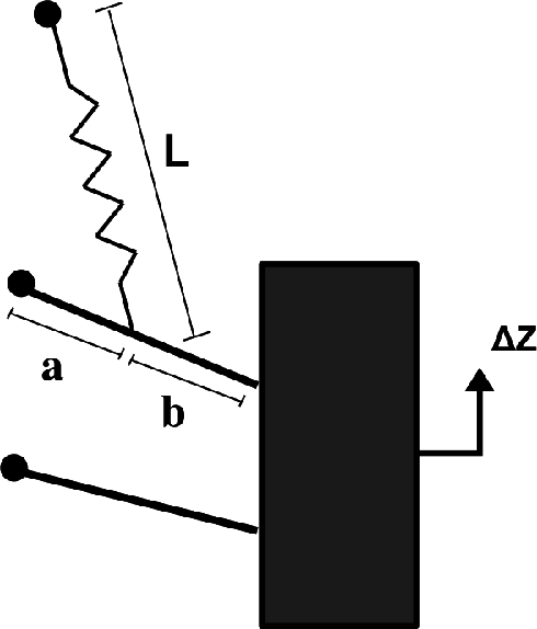
Neglecting any lever arm effects (
i.e., the kinematic displacement between the center of gravity and the sensor location), the measurement matrix
H is:
For the closed-loop error state navigation EKF, all of the states, except the attitude states of the state vector,
x, need to be fed back following the measurement update prior to the mechanization phase. For example, the update to the position state is given in
Equation (48):
where the superscripts + and
− represent before and after the error state corrections are applied and
represents the position error state estimate from the measurement update. The attitude errors,
, are corrections to the rotation matrix,
, and therefore cannot simply be added to the previous Euler angle estimates. The attitude states are updated by executing the following equations:
The Euler angles are then extracted from
by:
where
cij represents the element in the
i-th row and
j-th column of the rotation matrix
. Once the update is complete, the Kalman filter state vector,
, is reset to zero and
is used to initiate another time update cycle [
14].


