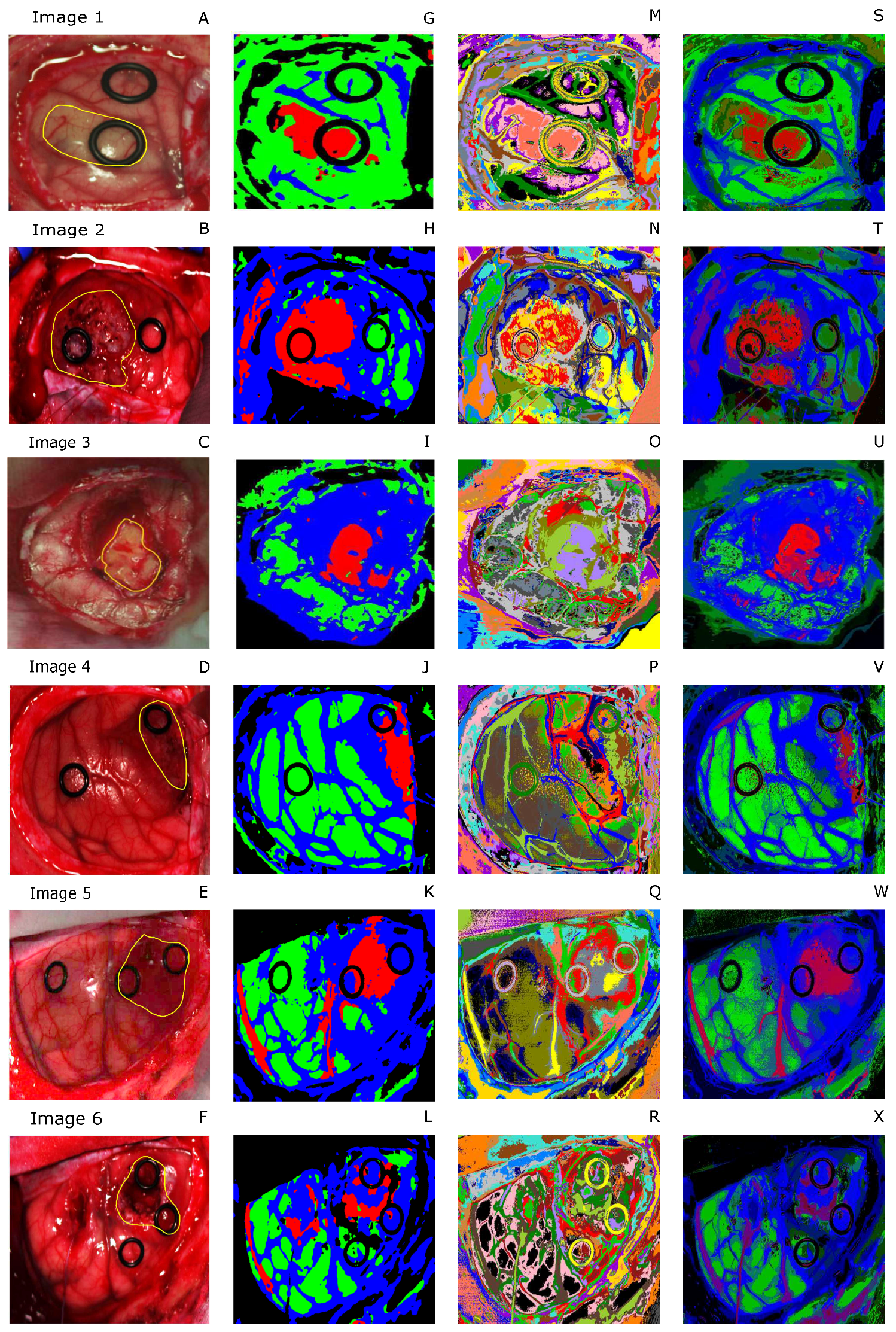
To graphically analyze the classification results,
Figure 5A–F shows the RGB images where the tumor is highlighted. Moreover,
Figure 5G–L depicts the supervised classification maps where the tumor is indicated with the red color, the healthy tissue in green, the hypervascularized in blue and the background in black. Images in
Figure 5M–R are the segmentation maps produced by the K-means algorithm. As can be seen from the images, this algorithm is capable of distinguishing blood vessels, different tissue regions and the ring markers (used by neurosurgeons to label the image for the supervised classification). As said before, the algorithm defines with high accuracy the boundaries of each area, but the clusters do not correspond to specific classes. Moreover, colors are randomly assigned to each cluster. For this reason, it is crucial to combine this segmentation map with the supervised classification result in obtain the final output, shown in
Figure 5S–X.
4.1. OpenMP Performance Evaluation
First, for each OpenMP implementation, several tests have been conducted in order to establish the optimal number of threads to be generated, using the biggest image (Image 6). These tests have been performed on an Intel i7 6700 processor working at 3.40 GHz equipped with 32 GB of RAM. The codes have been compiled with the
vc140 compiler, using compilation options to indicate the target architecture (i.e., x64 processor) and to maximize the processing speed. The processing times have been measured through the
omp_get_wtime routine. The obtained results are shown in
Figure 6.
It is important to highlight that the experiments have been conducted with the same initialization, and they provide the same number of iterations and the same classification results. For the first OpenMP implementation, we measured the processing time from 4 to 28 threads. We did not test the application with more threads since the processing time begins to significantly grow after 28 threads. By analyzing
Figure 6a, it is possible to see that the optimal number of threads for the first OpenMP version is 16. These measures have also been performed for the second OpenMP version, but in this case the maximum number of threads tested was 12 since the processing times begins to grow. In this case, as highlighted by
Figure 6b, the optimal number of threads is 8.
After establishing the optimal number of threads, we tested the two OpenMP versions on the entire dataset presented in
Table 1. In order to allow a direct comparison between the serial and the parallel versions, we initialized the algorithm with the same values for a given image. The obtained results, together with the speed-up values, are reported in
Table 2, where OpenMPv1 indicates the first version (the parallelization of the distance metric computation), while OpenMPv2 indicates the second one (the whole main loop parallelized). Those results, together with the others obtained by the CUDA and OpenCL versions, will be discussed in
Section 4.4.
4.2. CUDA Performance Evaluation
The three CUDA versions have been compiled using the NVIDIA
nvcc compiler, which is part of the CUDA 9.0 environment. Compilation options have been chosen in order to maximize the execution speed. The tests have been conducted using two different GPUs. The first one is a NVIDIA Tesla K40 GPU equipped with 2880 CUDA cores working at 750 MHz and with 12 GB of DDR5 RAM. It is based on the Kepler architecture that does not have a graphical output port since it is optimized for scientific computations. The second GPU is a NVIDIA GTX 1060 equipped with 1152 CUDA cores working at 1.75 GHz and with 3 GB of DDR5 RAM. This GPU is more recent than the first one and it is based on the Pascal architecture, having a graphical output port. In order to take full advantage of the specific architecture of each GPU, we indicate to the compiler which is the target micro-architecture. Specifically, we used the options
sm_35 and
compute_35 for the Tesla K40 GPU and the options
sm_60 and
compute_60 for the GTX 1060, where the values 35 and 60 represent the Kepler and the Pascal architecture, respectively. The results obtained using the Tesla K40 GPU are reported in
Table 3, while the results obtained by the GTX 1060 GPU are reported in
Table 4.
In both tables, CUDAv1 indicates the version where only the distance computation is computed on the GPU, CUDAv2 indicates the version where all the operations are performed in parallel and, finally, CUDAv3 indicates the version exploiting dynamic parallelism.
Concerning the GPU implementation, we also conducted a profiling using the NVIDIA Visual Profiler. This tool allows to profile the code execution on GPU together with memory transfers, in order to evaluate the efficiency of the implementation.
Figure 7 shows the results obtained by profiling the Image 1 (the most demanding one) processing on the GTX 1060 with the CUDAv1 (a) and CUDAv2 (b) codes. Concerning the CUDAv2, in
Figure 7b the different kernels executions percentage on the GPU are detailed. Profiling of CUDAv3 is not shown since it is very similar to CUDAv2 as well as the code profiling on the NVIDIA Tesla K40 GPU.
4.4. Comparisons and Discussion
The OpenMP version that offers the better results is the one where only the distance evaluations are processed in parallel. In this version, a parallel region is created and then destroyed at every iteration of the main loop, while in the second version the parallel region is created only once before the beginning of the main loop and is destroyed after the end of the main loop. However, the second version requires synchronization barriers between the threads, since there are operations that should be performed sequentially to obtain correct results. As an example, the increment of the number of iterations and the check of the conditions for repeating or not the main loop should be performed by a single thread. This is a critical issue since the advantage of creating and destroying the parallel region only once is thwarted by the synchronization bottleneck. The result analysis shows that the processing times are very similar, but the processor manages better the first version (OpenMPv1). Moreover, the speed-up values of the two versions are similar. Finally, it is important to highlight that the considered processor is equipped with 4 physical cores and the obtained speed-up is always greater than . This means that the parallelization efficiency is close to the theoretical value.
Concerning the CUDA versions, by analyzing
Table 3 and
Table 4, it is possible to observe that, for both GPU boards, the first CUDA version (CUDAv1) performs worse than the OpenMP ones. The reason is highlighted in
Figure 7a, where the profiling results show that the memory transfers take about 42% of the time and only the remaining 58% is used for the computation. This is the typical bottleneck of GPU computing since the memory transfers are performed by the PCI-express external bus. The second CUDA version (CUDAv2) is not affected by this issue since the amount of data transferred at each main iteration is significantly lower than in the previous case. It is possible to parameterize the amount of transferred data at each iteration for these two versions. In the first case (CUDAv1), the data transferred is the
matrix, which is made up of
elements represented in single precision floating-point arithmetic, while in the second case (CUDAv2) only one single precision floating-point value is copied back to the host. In the third case (CUDAv3), when dynamic parallelism is used, there are no data transfers inside the main loop. Therefore the third CUDA version is the one which transfers the minimum possible amount of data, but it does not perform better than the second version. This is because the dynamic parallelism produces an overhead due to the GPU switch between the main kernel and the subroutine kernel. This overhead affects every sub-kernel activation. In this specific case, four different sub-kernels are activated at every iteration. This overhead is not negligible and, as it can be seen form the results of
Table 3 and
Table 4, it takes longer than the copy of a single float value from device to host. In other words, the time needed by the GPU to manage the generation of four sub-kernels (CUDAv3) is comparable with the time taken by a single value copy from the host to the device memory (CUDAv2). Finally, for all the CUDA versions, the GTX 1060 board performs better than the Tesla K40, even if the last board is optimized for scientific computations. This is because the first board is equipped with a more recent architecture which has better CUDA cores working at a higher frequency than the Tesla GPU.
The analysis of the OpenCL versions highlight that, considering the Intel i7, the processing times are close to the OpenMP ones. For what concerns the Intel HD 530 integrated GPU, the performance is very poor, and the speed-ups are negligible. This is probably due to the low-end integrated GPU with a working frequency of 350 MHz and only 16 parallel processing elements. Therefore, it is not possible to obtain a significant speed-up compared to the serial version. Comparing the OpenCL version and the CUDA versions running on the GTX 1060 GPU, it is possible to notice that the OpenCL version performs better than the CUDAv1, but is significantly slower than the other two CUDA versions. These CUDA versions (CUDAv2 and CUDAv3) employ highly optimized routines, which exploits all the hardware features of a GPU. Moreover, the CUDA versions have been compiled using compilation options in order to produce an executable code which fully exploits the specific target architecture. This is not possible in OpenCL since it targets portability between different devices as main feature.
We also performed a comparative study between the three best performing versions of the three considered technologies in order to characterize how the speed-up varies with respect to the number of clusters. In particular, we performed experiments using Image 6 and
K values varying from 2 to 50. The speed-ups of the OpenMP, CUDA and OpenCL best versions with respect to the serial implementation are shown in
Figure 8 using a semi-logarithmic scale. It is possible to see that the CUDA version has a speed-up that ranges from
to ~
and from 12 clusters on it becomes nearly constant. On the other hand, the solutions based on a multi-core processor have speed-ups that are close to
.
In the literature, there are different works about parallel K-means.
Baramkar et al. [
18] performed a review of different parallel GPU-based K-means, but the considered works where focused only on general classification, without considering high data dimensionality, which is the case explored in our work. Therefore it is hard to perform direct comparisons with these works, which achieve very different speed-ups ranging from
to
.
Zechner et al. [
19] proposed a parallel implementation of this algorithm using both CPU and GPU. In particular, the GPU was only employed for distance computation, while centroids update was left to the CPU. They classified an artificial dataset with two-dimensional elements ranging from 500 to
. The maximum speed-up achieved was
, lower than the one obtained in our work. This is because the optimization proposed in [
19] is only valid for low-dimensional data and cannot be employed for classifying high-dimensional data such as hyperspectral images.
A similar approach is shown in [
20,
21], with the difference that also the clusters update has been performed on the GPU. However, between the distance computation and centroids update they performed host computation for updating each pixel label. This choice leads to a maximum speed-up of 60 in both works, lower than our one, since we moved all the computation on the device side.
In [
22], a GPU-based K-means algorithm is proposed, with a distance computation that is evaluated through a simple Cartesian distance. Under this assumption, they classify 1,000,000 pixels with 32 features in
s. In our case, the bigger image has 264,408 pixels, the features (i.e., the bands) are 128 and it is processed in ~
s. Moreover, the distance metric that we adopt (the spectral angle) is more complex than the one proposed in [
22].
Baydoun et al. [
23] developed a parallel K-means for RGB images classification. They adopted as metric a simple Cartesian distance and they parallelize only this computation, achieving a maximum speed-up of ~
. In this case, the metric and the data dimensionality are very different compared to this work.
In [
24], the K-means algorithm was modified to further reduce the distance computation. The speed-up varies from
to
, but also, in this case, it is not possible to perform a direct comparison since there are not enough details about the dataset composition. Finally, in [
25], the K-means algorithm was developed on GPU with the Cartesian distance. They adopt a modern GPU with 1536 CUDA cores obtaining a maximum speed-up of 88×, which is very similar to our results.
Lutz et al. [
26] proposed a parallel K-means implementation using an NVIDIA GTX 1080 GPU. They perfomed only experiments producing four groups and no further details are given in the paper about the dataset. They achieved a maximum speed-up of
which is nearly an order of magnitude smaller than one of our implementations.
A comparative analysis similar to the one we conducted is reported in [
27]. Authors exploited GPUs, OpenMP, Message Passing Interface (MPI) and FPGAs. However, also in this case, they considered only a dataset made up of 10-dimensional points, therefore the computational complexity of the distance computation is lower than our one. On the other hand, the results were not as good as our ones, since the maximum GPU speed-up achieved is ~
. They also demonstrated that the speed-up could reach a value up to
if the number of clusters to produce was significantly increased (i.e., more than 2000 clusters), but a study of how this speed-up varied also with respect to the data dimensionality were not carried out. Concerning OpenMP, the classification of 20,000 10-dimensionality points took ~3 s. Our smallest image is 6 times bigger than this one and with a dimensionality 18 times greater than the one considered. Keeping this in mind, the performance of our best OpenMP version is quite similar to this one. Finally, concerning the FPGA implementation, experiments were reported only with a
9-dimensionality dataset. Classification time is ~100 ms, but, as stated in [
27], the FPGA resources, especially memory banks, were not enough to process bigger datasets. The authors of this work do not use external DDR memory, therefore, the FPGA performance is limited due to this design choice.
The comparison between our work and the literature is summarized in
Table 6.

 ,
, 


