Hardware Resource Analysis in Distributed Training with Edge Devices

Abstract

When training a deep learning model with distributed training, the hardware resource utilization of each device depends on the model structure and the number of devices used for training. Distributed training has recently been applied to edge computing. Since edge devices have hardware resource limitations such as memory, there is a need for training methods that use hardware resources efficiently. Previous research focused on reducing training time by optimizing the synchronization process between edge devices or by compressing the models. In this paper, we monitored hardware resource usage based on the number of layers and the batch size of the model during distributed training with edge devices. We analyzed memory usage and training time variability as the batch size and number of layers increased. Experimental results demonstrated that, the larger the batch size, the fewer synchronizations between devices, resulting in less accurate training. In the shallow model, training time increased as the number of devices used for training increased because the synchronization between devices took more time than the computation time of training. This paper finds that efficient use of hardware resources for distributed training requires selecting devices in the context of model complexity and that fewer layers and smaller batches are required for efficient hardware use.

1. Introduction

The number of Internet of Things (IoT) devices connected to cloud servers is growing, which increases the amount of data that needs to be processed by those servers [1]. Consequently, network response latency between cloud servers and IoT devices is increasing. To reduce latency, edge computing [2] can be applied for real-time calculation on a device that generates and collects data.

Recently, intelligent environments such as smart homes and smart factories that combine deep learning (DL) with edge devices are more common [3,4,5,6]. Offloading the calculation of the edge device to the server reduces the execution time of the DL application. However, edge devices with high-performance chipsets, such as quad-cores, enable DL applications to be handled locally. However, only the inference phase is executed locally, while the training phase is executed on the server [7]. The training phase requires significant hardware resources and time.

Training a DL model requires sending collected data from the edge device to the server. As security threats to edge computing systems increase, server dependence needs to be reduced [8,9]. This problem can be solved by applying distributed training to the edge devices [10,11]; this enables training with multiple devices without a server to update the weight values of the DL model.

Existing research proposes a method to reduce the model size to minimize the computation time and hardware resources used [12]. One study proposes to improve the synchronization time between devices in the training phase in a mobile environment [13]. These studies focus on improving model-training time or reducing communication latency. Edge devices have limited hardware resources; thus, excessive hardware resources can be a bottleneck when training a model. Also, the hardware resource usage characteristics of each device depend on the number of devices and model configuration for distributed training. Existing studies do not consider the efficiency of hardware resource usage of edge devices. Based on the model and device configurations, we monitored the hardware usage required for training and demonstrated how to use the hardware efficiently.

We trained LeNet [14] and ResNet [15] with distributed training on ten Raspberry Pi 3 Model B boards. We demonstrated that to make efficient use of the hardware resources of the edge device, it was necessary to construct a small batch with fewer model layers. This configuration reduced training time by more than 300% and increased training accuracy by approximately 2%. We monitored central processing unit (CPU) utilization, memory usage, and network packets transmitted by each device during training and confirmed our efficient model configuration for training.

Furthermore, we monitored hardware resource usage while varying the number of layers, batch size, and the number of devices used for training. The batch size did not affect the training time. As the number of layers increased, the training time increased by approximately 350%. As the number of devices increased for training LeNet, the training time increased rather than the calculation of the training phase due to the increase in synchronization overhead between devices. Consequently, when training LeNet, the CPU utilization decreased by approximately 10% as the number of devices for distributed training increased. In ResNet’s training, the computation time was approximately 1000% faster as the number of devices increased, but the training accuracy decreased by approximately 15%. ResNet’s training demonstrated a CPU utilization difference of less than 3% depending on the number of devices.

The contributions of this paper are as follows:

• We trained the DL model using distributed training on edge devices. We demonstrate that DL models can be trained locally on edge devices without offloading to the server.
• We demonstrated a hardware resource-efficient distributed training model configuration for resource-constrained edge devices. We monitored the hardware resources used during the training phase. Results find that distributed training with smaller batch sizes and fewer layer sizes reduces training time and increases accuracy.

The remaining parts of this paper are organized as follows. Section 2 explains distributed training. In Section 3, we describe our distributed training environment. Section 4 presents the experimental environment and analysis results for distributed training. Section 5 discusses related works and the paper concludes in Section 6.

2. Backgrounds

Figure 1 shows the DL model as presented in several devices. The parallelization method is divided into two types, namely data parallelization and model parallelization. Data parallelization separates the input data and sends it to each device for training the model, as shown in Figure 1a. Each device uses the same DL network to train the data, the accuracy of which is based on the splitting of the input data.

Model parallelization divides the network of the model into different parts and assigns them to each device, as shown in Figure 1b. Each device learns using the same input data, although the model code must be modified and assigned to each device. Hence, the accuracy of the training is based on the division of the model.

In distributed training, both synchronous and asynchronous methods are used to synchronize the training data between devices [10]. The synchronization method synchronizes the training data of each device at the end of the epoch. Thus, the accuracy of the model is enhanced with the repetition of the epoch, and the training accuracy of each device depends on the data distribution. In the synchronization method, waiting time is generated owing to a variation in the epoch completion time between devices. By contrast, the asynchronous method synchronizes each device at the end of the entire training phase. The training time is shorter than that of the synchronous method because synchronization does not occur at each epoch, which reduces the accuracy of the final model.

In this paper, data parallelization is used for the experiment as shown in Figure 1a. We aim to use the existing model without any modification and apply the synchronization method to improve the accuracy of the trained model.

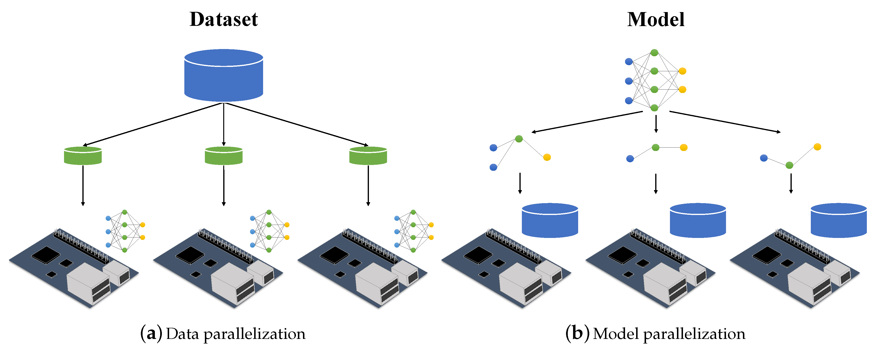
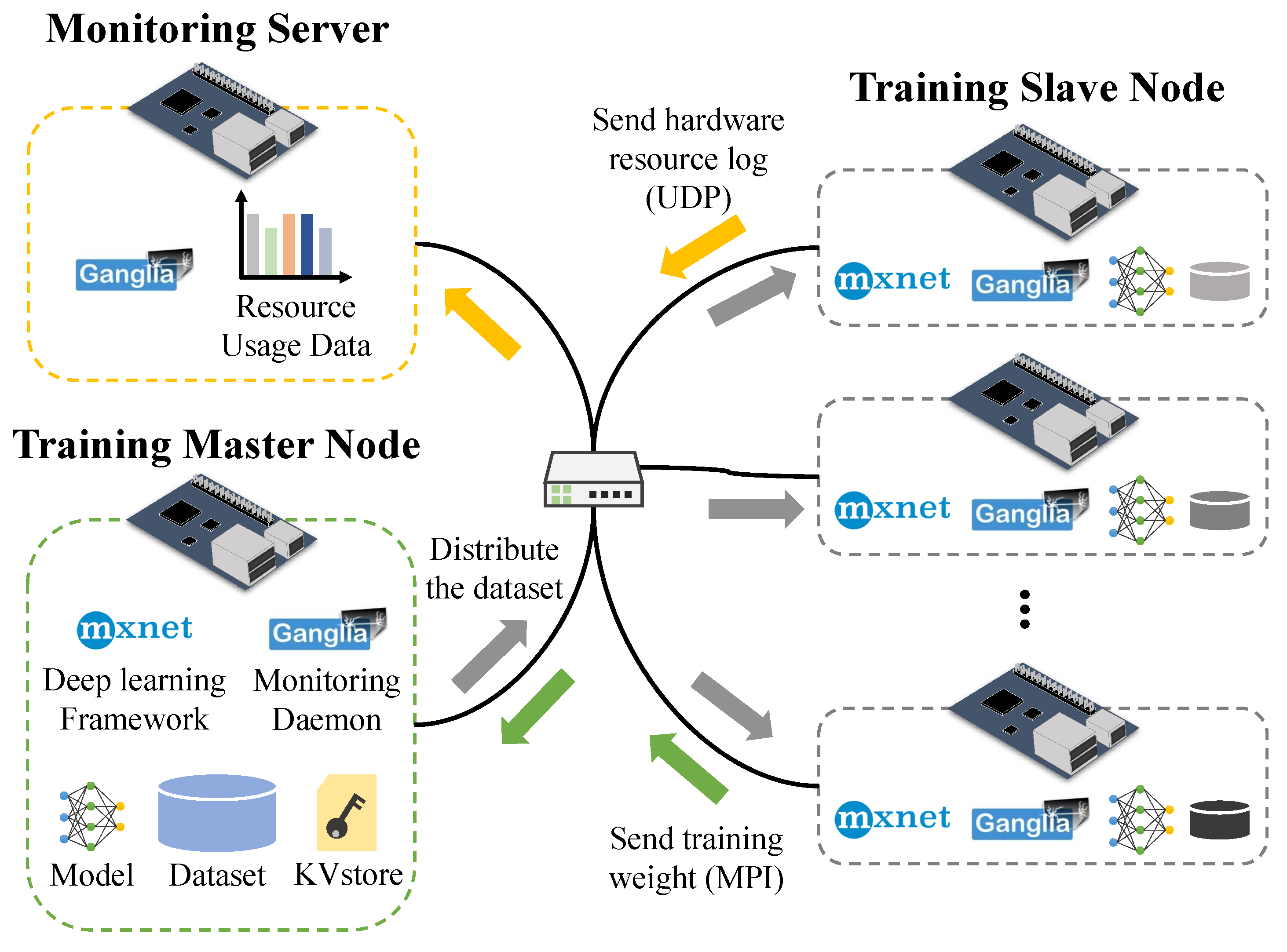
3. Distributed Training on Edge Devices

Figure 2 shows the configuration of an edge computing environment. It consists of a master node that stores the datasets and weights for distributed training, and a slave node that receives and trains the data. A monitoring server, which collects data on the hardware resource usage of each device, is present. Each device is connected to a 100 Mbps Ethernet.

The DL model undergoes distributed training using ten Raspberry Pi 3 Model B boards. Each board is composed of a 1.2 GHz quad-core CPU, 1 GB of memory, and a Linux 4.4 based Raspbian operating system.

The deep learning framework MXNet 0.9.5 [16] is used for distributed training. MXNet is preferably applied to edge devices owing to its small memory footprint [17]. MXNet uses a KVStore parameter server to update the model weight for synchronization, which is installed on all devices during distributed training. As discussed earlier, distributed training is carried out using data parallelization where each device communicates using a message passing interface (MPI). As the training begins, the master node is split and transmits the dataset to each slave node. Each slave node trains using the same model as the master node and sends the trained weights to the master node for synchronization between devices at the end of each batch.

Ganglia 3.7.2 [18] is used as the monitoring tool for the cluster environment to identify the CPU, memory, and network usage for training the model. The monitoring server device is further configured to collect the use of hardware resources for each device. Each edge device further sends the data to the monitoring server through the user datagram protocol (UDP) at 30 s intervals.

4. Evaluations

In this section, we describe the experimental environment and analyze the results of the model training through distributed training.

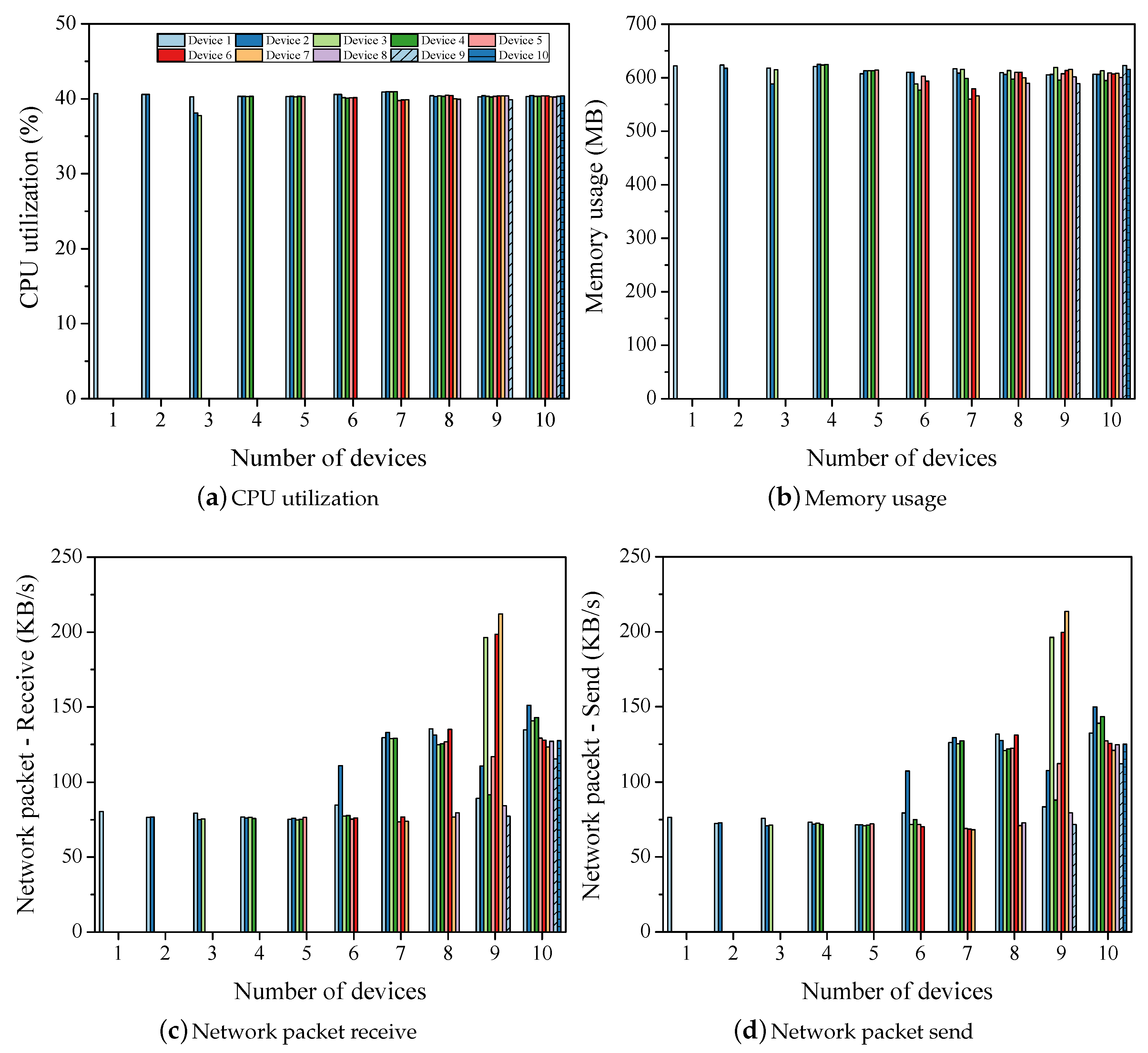
4.1. Experimental Environment

MNIST [14] and CIFAR-10 [15] datasets are used for the model training of LeNet and ResNet. Each dataset consists of 60,000 images. The MNIST dataset consists of $32\times 32$ monochrome images with handwritten numbers of 0–9, whereas the CIFAR-10 dataset has $32\times 32$ RGB images consisting of ten classes.

The LeNet is trained in two different manners, using either a multi-layer perceptron (MLP) [19] or a convolution neural network (CNN) [20]. In an MLP, several layers of a perceptron are connected sequentially. As a major disadvantage of an MLP, it flattens the image into a vector for an input of the first fully connected layer. This issue is resolved using a CNN through a structural representation of a weight. A CNN trains the features of the image through the convolution and pooling layers. The batch size is set to 64 for distributed training along with a mini-batch stochastic gradient descent (SGD) optimization.

ResNet helps resolve the gradient vanishing problem in deep depth networks [15] by connecting the input of the layer to its output through a residual block. ResNet comprises 152 layers for higher training accuracy. It is infeasible for Raspberry Pi 3 to train all layers of ResNet due to its low memory capacity. Approximately 17 GB of memory is required to train ResNet with 152 layers with 16 batch sizes [21]. Thus, the number of layers and the batch size of ResNet is set to match the target hardware. The numbers of layers and the batch sizes are set to 32, 80, and 110, and 32, 64, and 128, respectively. By contrast, LeNet comprises five layers. Therefore, it is possible to conduct training on the target board without any modification. As with LeNet training, we applied the SGD optimizer to the ResNet training.

The accuracy and time of training at each epoch is measured using this experiment. The effect of variance on the number of devices during distributed training is also examined. Thus, based on the characteristics of the model, the most efficient training method is determined.

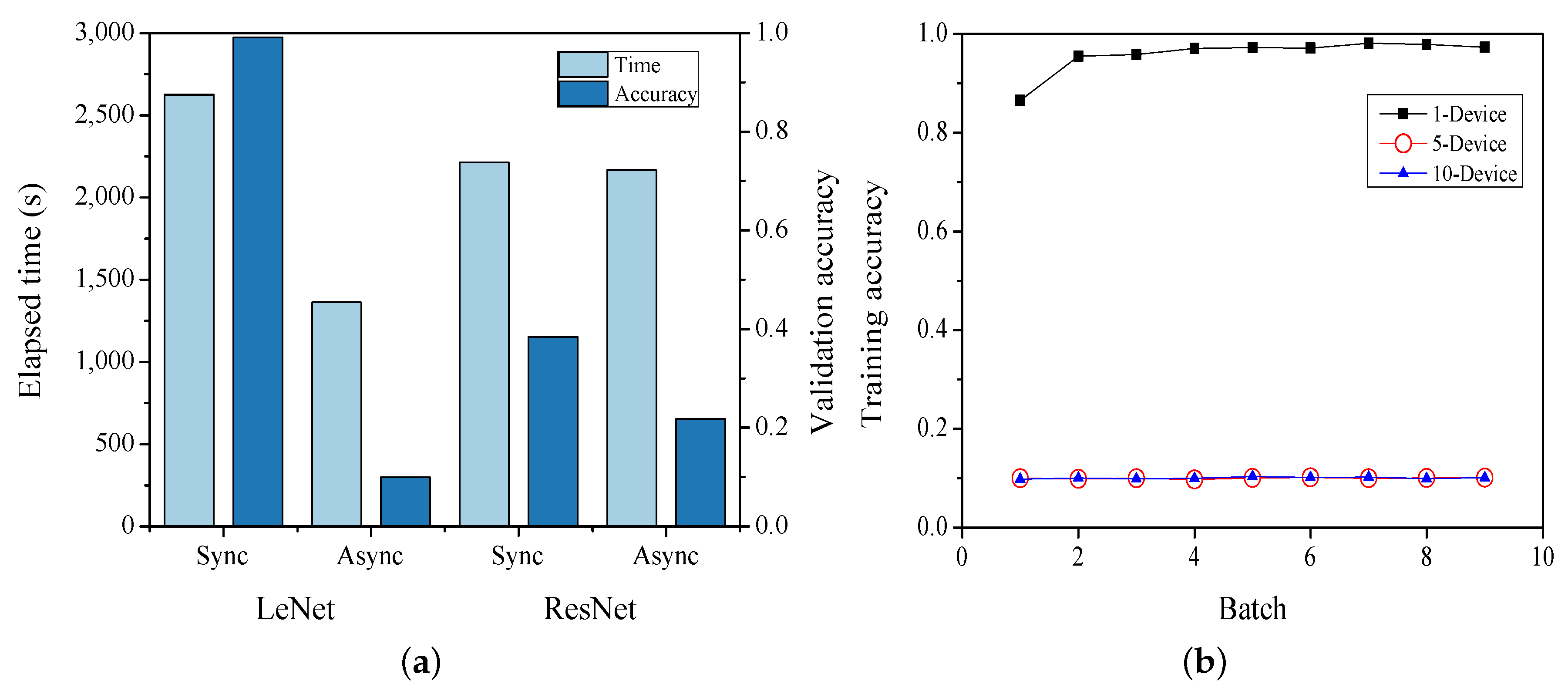
4.2. Comparison of Synchronization Method

As described in Section 2, there are two types of methods, namely synchronous and asynchronous, that synchronize the trained weights during distributed training. The training time and accuracy are measured based on each synchronization method during distributed training. Figure 3a shows LeNet and ResNet $32\times 32$ with ten devices to train one epoch using both synchronous and asynchronous methods. The figure shows the average value of each device during distributed training. The left Y-axis represents the training execution time and the right Y-axis represents the validation accuracy of the trained model. During LeNet training, the synchronous approach takes 1000 s more than the asynchronous approach. The training accuracy of the synchronous method is approximately 9-times higher than that of the asynchronous method. For ResNet, the training time for both the synchronous and asynchronous methods is approximately 2500 s. The training accuracy for the synchronous method is twice that of the asynchronous method.

Figure 3b shows the variance in accuracy at the time of asynchronous distributed training of LeNet when using one, five, and ten devices. When training a single device, an accuracy of 0.95 is observed from the first batch. By contrast, while training using five or ten devices, an accuracy of 0.1 is observed despite a repetition of batches. Thus, it can be stated that shallow models such as LeNet with asynchronous distributed training reduce the training time with lesser accuracy. In a deep model of distributed training such as ResNet, it was found that the synchronous method is time-efficient for homogeneous devices. In the case of heterogeneous devices, a synchronization method that considers the difference in the computing performance of the devices is required. Therefore, each model is trained using the synchronization method based on the above-mentioned results.

4.3. Experiment Results: LeNet

Table 1. Time and accuracy for training LeNet (multi-layer perceptron (MLP)).

	# of Devices
	1	2	3	4	5	6	7	8	9	10
Elapsed Time (s)	105	168	228	286	342	287	442	453	510	566
Validation Accuracy	0.961	0.971	0.970	0.970	0.975	0.974	0.974	0.974	0.973	0.971

illustrates the training results of LeNet using MLP. Training the model with a single device takes 105 s, and the verification accuracy is calculated to be 0.961. Depending on the number of devices, the training time increases by approximately 460 s when training with ten devices, and the training accuracy also increases.

Table 2. Time and accuracy for training LeNet (convolution neural network (CNN)).

	# of Devices
	1	2	3	4	5	6	7	8	9	10
Elapsed Time (s)	1079	1177	1338	1484	1778	2009	1970	2436	2665	2625
Validation Accuracy	0.982	0.988	0.989	0.990	0.990	0.991	0.989	0.990	0.990	0.991

lists the results when training LeNet using CNN. It takes 1079 s (≈18 min) to train with a single device and approximately 2625 s (≈45 min) with ten devices. The accuracy increases from 0.982 to 0.991. During LeNet training, a CNN is more accurate than an MLP by 0.02 because CNN exhibits less distortion while extracting the features of an image.

Figure 4 shows the use of hardware resources during the training phase. The X-axis of each graph represents the number of devices applied for training, and the Y-axis indicates the value of each item. As shown in Figure 4a, the CPU utilization is approximately 20% for a single device and 14% for an average of ten devices. During LeNet model training, the use of more devices increases the training time owing to a lesser utilization of the CPU. The design simplicity of LeNet makes it less efficient for use with multiple devices. LeNet comprises of five layers, which are classified into a small number of categories. The memory usage increases from approximately 300 to 330 MB as more devices are used, as shown in Figure 4b. In Figure 4c,d, no network usage is shown in distributed training using one or two devices. Model training with three or more devices requires over 1000 KB of network packets for synchronization. It was observed that more packets are generated with a longer training time. The results of the LesNet experiment indicate that training with more devices takes a longer time, whereas the training of lesser devices uses the hardware resources efficiently. The peak values shown in Figure 4c,d are due to an excess transmission when the device is in KVstore [16] during synchronization.

The experimental results indicate that shallow structures such as LeNet decrease the utilization of the CPU and increase the training time as more devices undergo distributed training.

4.4. Experiment Results: ResNet

The number of layers and batch sizes are varied to identify a suitable model for the efficient training of ResNet in Raspberry Pi. Figure 5 shows the time and accuracy of training based on the number of layers and the batch size, as well as the number of devices (denoted as $numberoflayers\times batchsize$). The X-axis represents the number of layers and the size of the batch, and the Y-axis represents the value of each item. In the case of a $32\times 32$ configuration, as shown in Figure 5a, the maximum training time for each device is 20,000 s (≈5 h) and the minimum is 2000 s. The maximum training time for $80\times 32$ and $110\times 32$ configurations is 50,000 s (≈14 h) and 80,000 s (≈22 h) and the minimum is 6000 and 8000 s, respectively. Here, a configuration of $110\times 128$ cannot be trained due to the low memory of Raspberry Pi. The accuracy for each case is calculated to be 0.49, 0.44, and 0.42, respectively, as shown in Figure 5b. The batch size does not affect the training time but does affect the training accuracy. As the batch size increases, the training accuracy decreases owing to a decrease in the number of synchronizations.

Figure 6 shows the hardware resources required to train ResNet with a $32\times 32$ configuration. The X-axis represents the number of devices for training, and the Y-axis is the value of each item. The utilization of the CPU decreases by 3% because it is training with a greater number of devices as compared to LeNet, as shown in Figure 4a and Figure 6a. The CPU utilization was calculated to be approximately 40% in most cases. The memory usage while training is calculated to be 280 MB for a single device and approximately 250 MB for ten devices, as shown in Figure 6b. ResNet requires 50 MB less memory for training than LeNet. During ResNet training, approximately 150 to 250 KB of packets are sent and received depending on the number of devices, as shown in Figure 6c,d. Training with LeNet requires nine synchronizations, whereas 72 are required with ResNet for a $32\times 32$ configuration. Therefore, the overall network usage is higher for training with ResNet as compared to that with LeNet.

To examine the effect of the number of layers and batch size on hardware utilization during distributed training, the layers and batches are set to 110 and 64, respectively. Figure 7 shows the usage of hardware resources for $110\times 64$ ResNet training. The CPU utilization (Figure 7a) is calculated to be approximately 40%, which is similar to that in the case of ResNet with $32\times 32$. The memory required for training ResNet with a $110\times 64$ configuration increases by approximately 2.5-fold to 600 MB owing to an increase in the batch size and the number of layers, as shown in Figure 7b. The training time increased by approximately 6-fold compared to that of ResNet with a $32\times 32$ configuration owing to the batch size and the number of layers, as shown in Figure 5a. The accuracy is slightly reduced, as shown in Figure 5b. Network packets sent (Figure 7c) and received (Figure 7d) for synchronization are reduced by up to 100 KB as compared to those in the case of ResNet with a $32\times 32$ configuration due to a decrease in the number of synchronizations and an increase in the batch size.

Table 3. Hardware resources by number of layers and batch size.

	Number of Layers × Batch Size
	$\mathbf{32}\times \mathbf{32}$	$\mathbf{32}\times \mathbf{64}$	$\mathbf{32}\times \mathbf{128}$	$\mathbf{80}\times \mathbf{32}$	$\mathbf{110}\times \mathbf{32}$
CPU utilization (%)	39.5	38.9	38.9	39.3	39.3
Memory usage (MB)	253.6	314.5	314.5	348.8	398.1
Network-receive (KB)	245.3	121.3	121.3	246.1	242.6
Network-send (KB)	245.7	119.6	119.6	250.8	243.7

shows the use of hardware resources based on the number of layers and batch size. The CPU utilization is calculated to be approximately 39%. When 32 layers are present in a model, a difference of 60 MB is observed based on the batch size. As the batch size increases, the packet transmission decreases by approximately 50%. In other words, as the number of synchronizations decreases, the accuracy decreases by 0.1, as shown in Figure 5b. When the number of layers is 80 and 110, the memory usage increases owing to an increase in the number of calculations, as compared to 32 layers. The packet transmission is observed to be similar.

Experiments show that a configuration of $32\times 32$ is required to train ResNet efficiently. Training with more devices reduces the training time by up to 90%, as shown in Figure 5a. The training accuracy decreases by approximately 0.1. As illustrated in

Table 4. Time and accuracy of ResNet $32\times 32$ with epoch iteration on ten devices.

	# of Epochs
	1	2	3	4	5
Elapsed time (s)	2212	4391	6598	8787	10,989
Validation accuracy	0.384	0.510	0.584	0.669	0.649

, it is possible to recover the accuracy by repeating the training of the epoch for half of the time. For distributed training on ten devices, the elapsed time after five epochs was calculated to be 10,989 s (≈3 h) with an accuracy of 0.649. Training with one device took approximately 5 h and provided an accuracy of 0.55. Previous experiments showed no significant change in the utilization of the CPU and memory based on the number of devices. Hardware resources can be made more efficient by iterating more epochs with ten devices.

5. Related Works

When the complexity and number of objects to be classified increase, distributed training [10] with multiple devices is used to train the deep neural network model.

Frameworks such as SINGA [22], Poseidon [23], and MXNet have been proposed for the distributed training of deep learning models. In addition, TensorFlow [24] and Caffe [25] can also be used for distributed training. The performance of distributed training frameworks has been studied on the high-performance computing (HPC) architecture, in a previous study [26]. This study analyzed the training time of Caffe, TensorFlow, and SINGA with respect to the CPU and GPU configurations in HPC, using an Intel Xeon and IBM Power 8 Processor. The results show that the training time of Caffe is approximately two times shorter than that of TensorFlow and SINGA, during the distributed training of GoogLeNet [27]. A performance analysis of the frameworks on the edge device was also performed [28]. In this study, inference tasks were performed on TensorFlow, Caffe2, PyTorch [29], and MXNet, using SqueezeNet [30], which is a lightweight model for mobile environments. Based on the experimental results, TensorFlow achieved the shortest training time on large CPU-based platforms. In contrast, Caffe2 achieved the shortest training time for the small-scale model. Additionally, PyTorch and MXNet were memory efficient and energy efficient at FogNode, respectively.

A previous study suggested a method to reduce the communication overhead between devices during distributed training on thousands of commodity off-the-shelf high-performance computers (COTS HPC) [31]. This study used MPI and InfiniBand to solve bottlenecks on GPUs between devices during distributed training. A study on distributed training using large-scale distributed GPUs provided a solution to the memory limitation, stalls, and data movement overhead of a GPU [32]. Using the proposed method, the training phase becomes more efficient with a parameter server that supports efficient memory management in data-parallel deep learning on distributed GPU devices. The effect remains constant while training on 108 CPUs with four GPUs.

Distributed training has been studied in both mobile and IoT environments. Personal information is important in a mobile environment because it contains sensitive user data. Federated learning (FL) [33,34] has been suggested as an approach to create a global model by training in a distributed manner in a mobile environment. The leakage of personal data is prevented by sending only trained weight from each mobile device. FL is an asynchronous method with a difference in accuracy between devices. In a heterogeneous network environment between mobile devices, it may take longer to upload a device with a slow network speed at the time the device-to-device synchronization process is applied. Federated training eliminates this overhead because no device-to-device synchronization occurs during the training process. An updating of the global model used in the device requires communication with the server. In one study, an extension of FL was proposed to efficiently manage client resources in a heterogeneous mobile environment [35]. This study proposes a synchronized node selection based on the hardware and communication resource constraints of a device during device-to-device synchronization through a protocol called Fed CS, reducing the Fashion-MNIST training time by approximately 33 min.

A study was conducted to optimize the synchronization time between devices in the distributed training of heterogeneous mobile systems [13]. In this study, a delay method is applied to the weight synchronization during the distributed training on heterogeneous devices, mobile devices, and servers. This suggests that synchronization should be carried out by considering the computational speed between nodes and configuring the system with three threads, namely, data distribution, a model update, and parameter communication. This reduces the training time by more than 3-fold compared to a parallel synchronization method. Another study proposed an adaptive periodic parameter averaging approach to reduce the communication overhead in distributed training on 16 GPUs [36]. This study applies adaptive SGD to reduce the bottleneck of a distributed SGD. Adaptive SGD reduces the communication time during distributed training by more than 500 s by automatically adjusting the average period of parallel SGD through data parallelism and parameter variance.

Recently, container-based virtualization has been applied to edge devices [37]. To achieve distributed learning on edge devices, the environment configured between the edge devices must be identical. Therefore, as the number of edge devices increases, the time required to build an environment also increases. To address this issue, a training environment for edge devices can be efficiently created by deploying a container environment.

6. Conclusions

Deep learning models are trained through distributed training on edge devices. It was proved that a distributed training configuration can apply hardware resources efficiently in an edge device. Thus, to use the hardware resources efficiently during distributed training, the number of layers in the model and the batch size should both be reduced. This configuration reduces the training time by 4-fold and increases the accuracy by 15%.

Both LeNet and ResNet were trained on ten Raspberry Pi boards. The shallow architecture of LeNet requires twice as much training time as compared to that required when it is trained with more devices, as the synchronization time between devices is longer than the computational time of the model. In the distributed training of ResNet, the training time is 10 times faster with 10 devices as compared to that with a single device. The training accuracy of the model is reduced by approximately 10%, owing to the variance of the input data. With distributed training, the variation in the number of devices does not significantly affect the CPU utilization or memory usage. The number of network packets required for device-to-device synchronization increases, along with a 100 MB increase in memory usage based on the number of layers in the model and the batch size.

References

1. Satyanarayanan, M. The emergence of edge computing. Computer 2017, 50, 30–39. [Google Scholar] [CrossRef]
2. Shi, W.; Cao, J.; Zhang, Q.; Li, Y.; Xu, L. Edge computing: Vision and challenges. IEEE Internet Things J. 2016, 3, 637–646. [Google Scholar] [CrossRef]
3. Manic, M.; Amarasinghe, K.; Rodriguez-Andina, J.J.; Rieger, C. Intelligent buildings of the future: Cyberaware, deep learning powered, and human interacting. IEEE Ind. Electron. Mag. 2016, 10, 32–49. [Google Scholar] [CrossRef]
4. Xu, K.; Wang, X.; Wei, W.; Song, H.; Mao, B. Toward software defined smart home. IEEE Commun. Mag. 2016, 54, 116–122. [Google Scholar] [CrossRef]
5. Chen, B.; Wan, J.; Shu, L.; Li, P.; Mukherjee, M.; Yin, B. Smart factory of industry 4.0: Key technologies, application case, and challenges. IEEE Access 2017, 6, 6505–6519. [Google Scholar] [CrossRef]
6. Candanedo, I.S.; Nieves, E.H.; González, S.R.; Martín, M.T.S.; Briones, A.G. Machine learning predictive model for industry 4.0. In Proceedings of the International Conference on Knowledge Management in Organizations, Zilina, Slovakia, 6–10 August 2018; pp. 501–510. [Google Scholar]
7. Li, H.; Ota, K.; Dong, M. Learning IoT in edge: Deep learning for the Internet of Things with edge computing. IEEE Netw. 2018, 32, 96–101. [Google Scholar] [CrossRef] [Green Version]
8. Wang, H.; Zhang, Z.; Taleb, T. Special issue on security and privacy of IoT. World Wide Web 2018, 21, 1–6. [Google Scholar] [CrossRef] [Green Version]
9. Jacobsson, A.; Boldt, M.; Carlsson, B. A risk analysis of a smart home automation system. Future Gener. Comput. Syst. 2016, 56, 719–733. [Google Scholar] [CrossRef] [Green Version]
10. Dean, J.; Corrado, G.; Monga, R.; Chen, K.; Devin, M.; Mao, M.; Ranzato, M.; Senior, A.; Tucker, P.; Yang, K.; et al. Large scale distributed deep networks. In Proceedings of the Advances in Neural Information Processing Systems, Lake Tahoe, CA, USA, 3–6 December 2012; pp. 1223–1231. [Google Scholar]
11. Teerapittayanon, S.; McDanel, B.; Kung, H.T. Distributed deep neural networks over the cloud, the edge and end devices. In Proceedings of the 2017 IEEE 37th International Conference on Distributed Computing Systems (ICDCS), Atlanta, GA, USA, 5–8 June 2017; pp. 328–339. [Google Scholar]
12. Rastegari, M.; Ordonez, V.; Redmon, J.; Farhadi, A. Xnor-net: Imagenet classification using binary convolutional neural networks. In Proceedings of the European Conference on Computer Vision, Amsterdam, The Netherlands, 8–16 October 2016; pp. 525–542. [Google Scholar]
13. Zhang, J.; Xiao, J.; Wan, J.; Yang, J.; Ren, Y.; Si, H.; Zhou, L.; Tu, H. A parallel strategy for convolutional neural network based on heterogeneous cluster for mobile information system. Mob. Inf. Syst. 2017, 2017, 1–12. [Google Scholar] [CrossRef] [PubMed]
14. LeCun, Y.; Jackel, L.; Bottou, L.; Cortes, C.; Denker, J.S.; Drucker, H.; Guyon, I.; Muller, U.A.; Sackinger, E.; Simard, P.; et al. Learning algorithms for classification: A comparison on handwritten digit recognition. Neural Netw. Stat. Mech. Perspect. 1995, 261, 276. [Google Scholar]
15. Krizhevsky, A.; Sutskever, I.; Hinton, G.E. Imagenet classification with deep convolutional neural networks. In Proceedings of the Advances In Neural Information Processing Systems, Lake Tahoe, CA, USA, 3–6 December 2012; pp. 1097–1105. [Google Scholar]
16. Chen, T.; Li, M.; Li, Y.; Lin, M.; Wang, N.; Wang, M.; Xiao, T.; Xu, B.; Zhang, C.; Zhang, Z. Mxnet: A flexible and efficient machine learning library for heterogeneous distributed systems. arXiv 2015, arXiv:1512.01274. [Google Scholar]
17. Zhang, K.; Alqahtani, S.; Demirbas, M. A comparison of distributed machine learning platforms. In Proceedings of the 2017 26th International Conference on Computer Communication and Networks (ICCCN), Vancouver, BC, Canada, 31 July–3 August 2017; pp. 1–9. [Google Scholar]
18. Massie, M.; Li, B.; Nicholes, B.; Vuksan, V.; Alexander, R.; Buchbinder, J.; Costa, F.; Dean, A.; Josephsen, D.; Phaal, P.; et al. Monitoring with Ganglia: Tracking Dynamic Host and Application Metrics at Scale; O’Reilly Media, Inc.: Sebastopol, CA, USA, 2012. [Google Scholar]
19. Gardner, M.W.; Dorling, S. Artificial neural networks (the multilayer perceptron)—A review of applications in the atmospheric sciences. Atmos. Environ. 1998, 32, 2627–2636. [Google Scholar] [CrossRef]
20. Lin, M.; Chen, Q.; Yan, S. Network in network. arXiv 2013, arXiv:1312.4400. [Google Scholar]
21. Wu, Z.; Shen, C.; Van Den Hengel, A. Wider or deeper: Revisiting the resnet model for visual recognition. Pattern Recognit. 2019, 90, 119–133. [Google Scholar] [CrossRef] [Green Version]
22. Ooi, B.C.; Tan, K.L.; Wang, S.; Wang, W.; Cai, Q.; Chen, G.; Gao, J.; Luo, Z.; Tung, A.K.; Wang, Y.; et al. SINGA: A distributed deep learning platform. In Proceedings of the 23rd ACM International Conference on Multimedia, Brisbane, Australia, 26–30 October 2015; pp. 685–688. [Google Scholar]
23. Zhang, H.; Zheng, Z.; Xu, S.; Dai, W.; Ho, Q.; Liang, X.; Hu, Z.; Wei, J.; Xie, P.; Xing, E.P. Poseidon: An efficient communication architecture for distributed deep learning on {GPU} clusters. In Proceedings of the 2017 USENIX Annual Technical Conference (USENIX ATC 17), Santa Clara, CA, USA, 12–14 July 2017; pp. 181–193. [Google Scholar]
24. Abadi, M.; Agarwal, A.; Barham, P.; Brevdo, E.; Chen, Z.; Citro, C.; Corrado, G.S.; Davis, A.; Dean, J.; Devin, M.; et al. Tensorflow: Large-scale machine learning on heterogeneous distributed systems. arXiv 2016, arXiv:1603.04467. [Google Scholar]
25. Jia, Y.; Shelhamer, E.; Donahue, J.; Karayev, S.; Long, J.; Girshick, R.; Guadarrama, S.; Darrell, T. Caffe: Convolutional architecture for fast feature embedding. In Proceedings of the 22nd ACM International Conference on Multimedia, Orlando, FL, USA, 3–7 November 2014; pp. 675–678. [Google Scholar]
26. Shams, S.; Platania, R.; Lee, K.; Park, S.J. Evaluation of deep learning frameworks over different HPC architectures. In Proceedings of the 2017 IEEE 37th International Conference on Distributed Computing Systems (ICDCS), Atlanta, GA, USA, 5–8 June 2017; pp. 1389–1396. [Google Scholar]
27. Szegedy, C.; Liu, W.; Jia, Y.; Sermanet, P.; Reed, S.; Anguelov, D.; Erhan, D.; Vanhoucke, V.; Rabinovich, A. Going deeper with convolutions. In Proceedings of the IEEE Conference on Computer Vision and Pattern Recognition, Boston, MA, USA, 7–12 June 2015; pp. 1–9. [Google Scholar]
28. Zhang, X.; Wang, Y.; Shi, W. pcamp: Performance comparison of machine learning packages on the edges. In Proceedings of the USENIX Workshop on Hot Topics in Edge Computing (HotEdge 18), Boston, MA, USA, 11–13 July 2018. [Google Scholar]
29. Paszke, A.; Gross, S.; Massa, F.; Lerer, A.; Bradbury, J.; Chanan, G.; Killeen, T.; Lin, Z.; Gimelshein, N.; Antiga, L.; et al. PyTorch: An imperative style, high-performance deep learning library. In Proceedings of the NIPS 2019—Neural Information Processing Systems, Vancouver, CO, Canada, 10–12 December 2019; pp. 8024–8035. [Google Scholar]
30. Iandola, F.N.; Han, S.; Moskewicz, M.W.; Ashraf, K.; Dally, W.J.; Keutzer, K. SqueezeNet: AlexNet-level accuracy with 50× fewer parameters and <0.5 MB model size. arXiv 2016, arXiv:1602.07360. [Google Scholar]
31. Coates, A.; Huval, B.; Wang, T.; Wu, D.; Catanzaro, B.; Andrew, N. Deep learning with COTS HPC systems. In Proceedings of the International Conference on Machine Learning, Atlanta, GA, USA, 16–21 June 2013; pp. 1337–1345. [Google Scholar]
32. Cui, H.; Zhang, H.; Ganger, G.R.; Gibbons, P.B.; Xing, E.P. Geeps: Scalable deep learning on distributed gpus with a gpu-specialized parameter server. In Proceedings of the Eleventh European Conference on Computer Systems, London, UK, 18–21 April 2016; p. 4. [Google Scholar]
33. Konečnỳ, J.; McMahan, B.; Ramage, D. Federated optimization: Distributed optimization beyond the datacenter. arXiv 2015, arXiv:1511.03575. [Google Scholar]
34. Konečnỳ, J.; McMahan, H.B.; Yu, F.X.; Richtárik, P.; Suresh, A.T.; Bacon, D. Federated learning: Strategies for improving communication efficiency. arXiv 2016, arXiv:1610.05492. [Google Scholar]
35. Nishio, T.; Yonetani, R. Client selection for federated learning with heterogeneous resources in mobile edge. In Proceedings of the ICC 2019—2019 IEEE International Conference on Communications (ICC), Shanghai, China, 20–24 May 2019; pp. 1–7. [Google Scholar]
36. Jiang, P.; Agrawal, G. Accelerating distributed stochastic gradient descent with adaptive periodic parameter averaging: poster. In Proceedings of the 24th Symposium on Principles and Practice of Parallel Programming, Washington, DC, USA, 16–20 February 2019; pp. 403–404. [Google Scholar]
37. Morabito, R. Virtualization on internet of things edge devices with container technologies: A performance evaluation. IEEE Access 2017, 5, 8835–8850. [Google Scholar] [CrossRef]
Figure 1. Parallelization method of distributed training.
Electronics 09 00028 g001
Figure 2. Distributed training environment.
Electronics 09 00028 g002
Figure 3. Training results in synchronous and asynchronous method. (a) Comparison of time and accuracy according to synchronization method. (b) Accuracy in asynchronous distributed training of LeNet.
Electronics 09 00028 g003
Figure 4. Hardware resources for training LeNet (CNN).
Electronics 09 00028 g004aElectronics 09 00028 g004b
Figure 5. ResNet training time and accuracy by number of layers and batch size (1 epoch).
Electronics 09 00028 g005
Figure 6. Hardware resources for training ResNet 32 × 32 .
Electronics 09 00028 g006
Figure 7. Hardware resources for training ResNet 110 × 64 .
Electronics 09 00028 g007