The Language of Spheres in Physics

Abstract

Physical laws manifest themselves through the amalgamation of mathematical symbols, numbers, functions, geometries, and relationships. These intricate combinations unfold within a mathematical model devised to capture and represent the “objective reality” of the system under examination. In this symbiotic relationship between physics and mathematics, the language of mathematics becomes a powerful tool for describing and predicting the behavior of the physical world. The language used and the associated concepts are in a perpetual state of evolution, mirroring the ongoing expansion of the phenomena accessible to our scientific understanding. In this contribution, written in honor of Richard Kerner, we delve into fundamental, at times seemingly elementary, elements of the mathematical language inherent to the physical sciences, guided by the overarching principles of symmetry and group theory. Our focus turns to the captivating realm of spheres, those strikingly symmetric entities that manifest prominently within our geometric landscape. By exploring the interplay between mathematical abstraction and the tangible beauty of symmetry, we seek to deepen our understanding of the underlying structures that govern our interpretation of the physical world.

1. Introduction

This contribution serves as a friendly tribute to Richard Kerner, a distinguished figure in the realm of theoretical and mathematical physics, whose methodologies consistently embody a harmonious blend of precision, intuition, and a poetic touch. Kerner’s ability to reveal the concealed facets of diverse phenomena, in the domains of general relativity and gauge theory (Kaluza–Klein, e.g., [1]), condensed matter (glasses, e.g., [2]), particle physics (quarks and ternary algebras, e.g., [3]), noncommutative geometric structures (e.g., [4]), and many others, is an attestation of his profound insights.

In each of his works, Kerner consistently imparts that distinct touch of originality, elevating his contributions beyond the ordinary. His dedication to unraveling the intricacies of the universe is reflected not only in the rigor of his approach but also in the elegance with which he brings to light the hidden dimensions of our physical reality. One of his latest publications, as referenced in [5], stands as a magisterial testament to his multifaceted talents.

This current contribution aligns seamlessly with the theme encapsulated in the title The Languages of Physics of the special issue in honor of Kerner. My focus will be directed towards the mathematical language of physics, emphasizing the inherent limitation in precision when scrutinized from the perspective of a physicist. Such models are transient rather than eternal, subject to the passage of (entropic) time and contingent upon the scale at which they operate. To align with experimental observations and predictions, these models often undergo modifications, sometimes requiring radical transformations. In the dynamic interplay between the modeler and the modeled object, a degree of probability emerges, representing the level of epistemic confidence in the model’s appropriateness [6].

This recognition of inherent uncertainty gives rise to the imperative of introducing some level of coarse-graining into the initial mathematical model, conceived to portray an ontic entity or fact. Take, for example, the inconceivability of irrational numbers in human perception, conceivability being here understood in terms of a measurable physical quantity. Yet physical laws, for several centuries now, have been articulated in terms of real numbers, denoted as $\mathbb{R}$, constructed from the abstract concept of limits (such as the limit of Cauchy sequences of rational numbers).

Nevertheless, these profoundly abstract mathematical concepts have evolved to such a degree of familiarity that they now stand as an indispensable foundation for formulating descriptions of our environment. Serving as a robust backdrop, they assist us in imposing structure and establishing a set of physical laws capable of navigating the intricacies of complexity and chaos. In our pursuit of order, we inevitably organize observations through the lens of symmetry.

Beneath the allure of this aesthetic concept lies the intricate framework of mathematics, particularly the concept of a group, with all its potential generalizations, deformations, approximations, and the inherent challenges of incompleteness and partial versions. It is within this mathematical tapestry that we find the tools and principles allowing us to not only conceptualize but also articulate the laws that govern the universe, providing a coherent and profound understanding of our complex reality.

In this contribution, which draws inspiration from a previous review [7] and recent lectures held in both Poland and Brazil, serving as a significant element within the thematic framework of the special issue titled “The Languages of Physics”, we harness the potency of the concept of symmetry to reexamine the first elements of the sequence of unit spheres, denoted as ${\mathbb{S}}^n$, and explore their profound physical implications across various domains of physics. This exploration extends into realms such as atomic, molecular, nuclear, particle, and condensed matter physics, shedding light on the intricate interplay between the mathematical abstraction of spheres and their tangible relevance in understanding the fundamental structures and behaviors that underpin the diverse facets of the physical world. In this regard, I cannot resist quoting the following excerpt from [8], translated from French.

From there comes her fascination for pieces, lids, and other wheels whose circular movement she perpetuates, immersed in a hypnotic contemplation that extracts her from the world and disconnects her from a reality that is too aggressive.

We do not aspire to introduce entirely original content in this paper. Rather, it is conceived as a fusion of fundamental (somewhat very basic) and advanced discussions on the mathematics of symmetry. Rather than striving to introduce entirely novel content, this article is crafted as a synthesis, merging fundamental (yet foundational) discussions with advanced insights into the mathematics of symmetry.

The journey begins with a recapitulation of essential concepts pertaining to groups and semi-groups (Section 2), followed by a freshman level reminder of algebraic and topological aspects of numbers (Section 3). We then show the significant role played by simple or semisimple Lie groups in elucidating symmetries across classical and quantum physics realms (Section 4).

The core of this presentation centers on a reexamination of the realm of spheres (Section 5) and the ensuing exploration of the associated geometry of Hopf fibrations (Section 6). Furthermore, we unravel the mesmerizing simplifications that the spherical symmetry contributes to explaining the Balmer lines, detailing the spectral line emissions of the hydrogen atom—a proto-quantum formalism dating back to 1885 (Section 7). The paper concludes with a succinct summary in Section 8.

For those seeking a more in-depth understanding, Appendix A and Appendix B provide additional details on group actions and the Lie algebra formalism.

2. Semi-Groups and Groups

In this section we recap main definitions concerning semi-groups, groups, and structures built from them. Usually these notions are supposed known but reviewing them lies in the self-contained spirit of this contribution.

2.1. Definitions

A semi-group is a set $G=\{g\in G\}$ equipped with an operation that combines any two elements $g_1\in G$ and $g_2\in G$ to form a third element $g_3=g_1{g}_2\in G$ while being associative, i.e., $\left(g_1{g}_2\right)g_3=g_1\left(g_2{g}_3\right)\equiv g_1{g}_2{g}_3$.

A group is a semi-group having an identity element e, $eg=ge=g$ and inverse elements, $g^{-1}g=g{g}^{-1}=e$.

A group or semi-group is Abelian if the operation is commutative: $g_1{g}_2=g_2{g}_1$ for all $g_1,g_2\in G$, e.g., translations in the line or to rotations on the circle or in the plane. Rotations in space are noncommutative.

Groups can be finite (e.g., permutations, point groups of symmetry of molecules), discrete (e.g., space group of symmetry of crystals), continuous (e.g., Euclidean displacements), Lie groups (infinitesimal transformations can be considered as well).

Continuous groups can be compact (parameters of transformation are bounded, e.g., rotations on the sphere) or non-compact, e.g., translations in the plane.

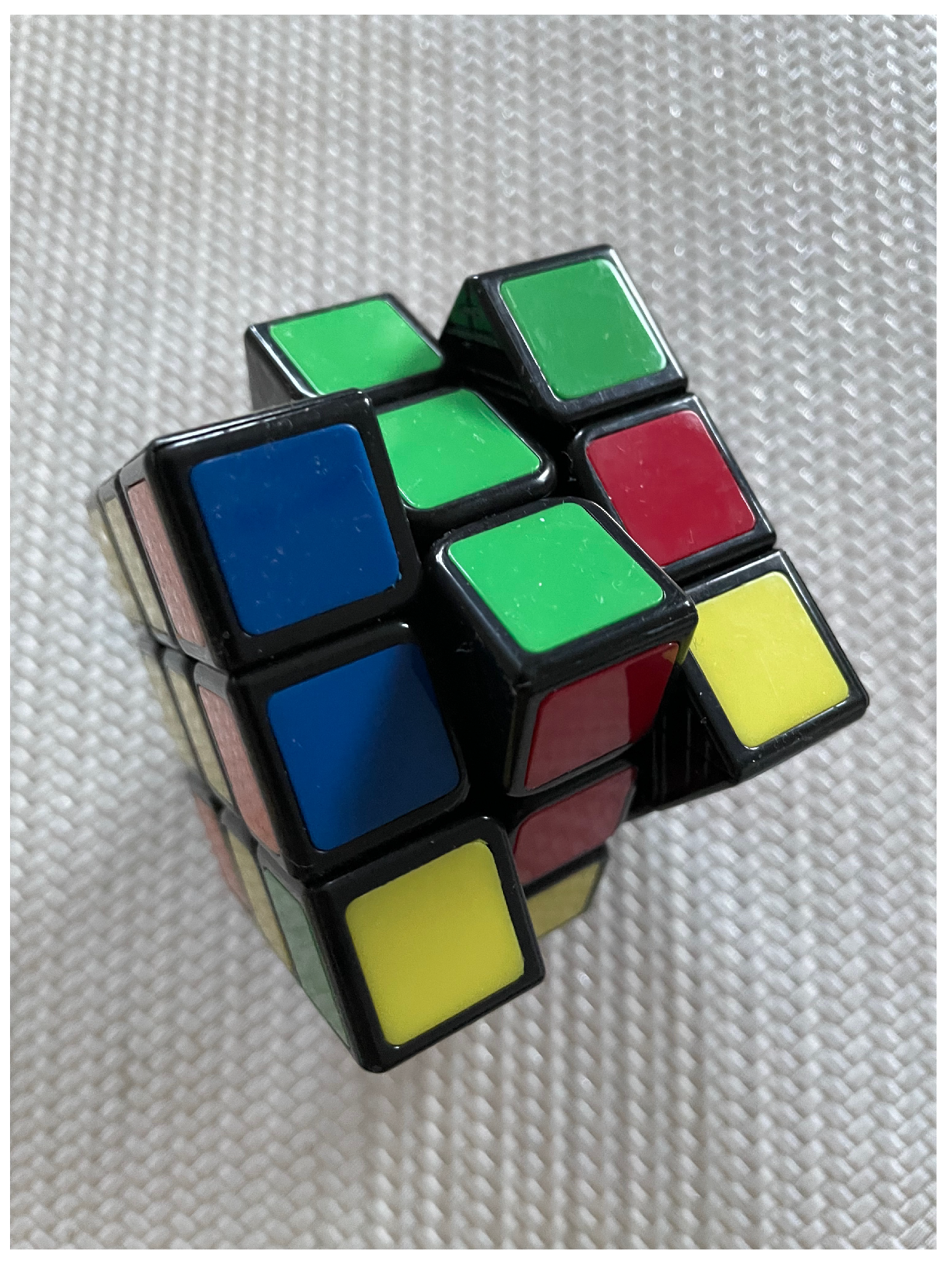
Two elements $g_1$ and $g_2$ of a group G are said to be conjugate if there exists $g\in G$ such that $g_2=g{g}_1{g}^{-1}$. This is an equivalence relation whose equivalence classes are called conjugacy classes (one famous example is the Rubik cube where the essential property for winning is precisely the set of conjugate classes of one permutation group, see Figure 1 and [9] for explanation).

2.2. Example: Chirality

Chirality is the simplest example of a group: $G=\{I,P\}$, with $IP=PI=P$, $I^2=I=P^2$. P is like a mirror image. A figure is chiral if it cannot be mapped to its mirror image by rotations and translations alone. Examples are shown in Figure 2 and Figure 3.

A chiral object and its mirror image are said to be enantiomorphs.

An interesting question about mirrors is shown in Figure 4: why does a mirror reverse left to right, but not top to bottom?

Beyond space parity (usually noted P), notable similar instances are observed in the realm of particle physics. These include charge conjugation (C), where the charge of a particle is reversed ($q\leftrightarrow -q$), time reversal (T), involving the reversal of time ($t\leftrightarrow -t$), and the dichotomy between matter and antimatter. Furthermore, the interplay of these individual symmetries gives rise to intriguing combinations such as $PT$, $CP$, and $CPT$, adding depth and complexity to our understanding of fundamental physical principles.

2.3. Building Groups from Subgroups

A subset H of a group G is a subgroup of G if it contains e and is stable versus group operations: $HH:=\{h_1{h}_2,h_1,h_2\in H\}\subset H$ and $H^{-1}:=\{h^{-1},h\in H\}\subset H$. The direct product of two groups $G_1$ and $G_2$ consists in gluing the two groups together, without interaction: $G=G_1\times G_2$ is simply their Cartesian product, endowed with the group law:

$$(g_1,g_2)(g_1^{\prime },g_2^{\prime })=(g_1{g}_1^{\prime },g_2{g}_2^{\prime }),g_1,g_1^{\prime }\in G_1,g_2,g_2^{\prime }\in G_2.$$

The neutral element is $(e_1,e_2)$. With the identifications $g_1\sim (g_1,e_2),g_2\sim (e_1,g_2)$, both $G_1$ and $G_2$ are invariant subgroups of $G_1\times G_2$ (think of the plane as the product of two lines or of the torus as the product of two circles).

For the semi-direct product of two groups $G_1$ and $G_2$, one supposes one is given a homomorphism $\alpha$ from $G_2$ into the group $\mathrm{Aut}{G}_1$ of automorphisms of $G_1$. Then, one defines the semi-direct product $G=G_1⋊G_2$ as the Cartesian product, endowed with the group law:

$$(g_1,g_2)(g_1^{\prime },g_2^{\prime })=(g_1{\alpha }_{g_2}\left(g_1^{\prime }\right),g_2{g}_2^{\prime })$$

The neutral element is $(e_1,e_2)$ and the inverse of $(g_1,g_2)$ is ${(g_1,g_2)}^{-1}=\left({\left[{\alpha }_{g_2^{-1}}\left(g_1\right)\right]}^{-1},g_2^{-1}\right)$ (think of the affine group of the line, which combines dilation and translation).

2.4. Group Cosets

Let H be a subgroup of G. One says that $g_1\equiv g_2$ mod H if there exists $h\in H$ such that $g_2=g_{1}h$. Denoting $\overline{g}=gH$ the equivalence class of g mod H, the set of equivalence classes is denoted $G/H$ and called the left coset of G by H. The right coset $H\setminus G$ is defined in a similar way as the set of equivalence classes $\{Hg,g\in G\}$.

2.5. Group Actions

Irreducibility linked to symmetry (and invariance) is the mathematical concept of a group, more precisely the group of transformations (see Appendix A for more details). Concretely, elements in a group G, like the group of Euclidean displacements in the plane (the semidirect product of rotations and translations), transform into themselves objects in a set X, like the set of triangles, in such a way that we can compose such transformations in an associative way and we can transform back too:

$$g\in G,x\in X,g·x=y\in X\iff x=g^{-1}·y,\left(g{g}^{\prime }\right)·x=g·(g^{\prime }·x)$$

3. Numbers and Groups

In this section we implement the group material exposed above through the sequence of numbers, from the most elementary ones to some sophisticated objects like octonions and Cayley algebras.

3.1. Sets $\mathbb{N}$, $\mathbb{Z}$, ${\mathbb{Z}}_p$

In preamble, one should remember that Arithmetic with (cardinal) Hindu–Arabic numerals is easy while it is inextricable with (ordinal) Roman numerals (e.g., Figure 5).

The set of natural numbers $\mathbb{N}:=\{0,1,2,3,\cdots \}$ (note that including 0 is now the common convention among set theorists and logicians, maybe not with artists’ assent, see Figure 6 and [12]) equipped with addition, is not a group (no inverse), just an Abelian semi-group. Equipped with multiplication, $\mathbb{N}$ is an Abelian semi-group as well.

The set of rational integers $\mathbb{Z}:=\{\cdots ,-3,-2,-1,0,1,2,3,\cdots \}=-{\mathbb{N}}^{*}\cup \mathbb{N}$, equipped with addition, is an Abelian group. Equipped with multiplication, it is a semi-group.

The set of rational integers modulo p, $p=2,3,\cdots$: ${\mathbb{Z}}_p=\{0,1,2,\cdots ,p-1,\mathrm{mod}p\}$, equipped with addition, is a finite Abelian group with p elements. Chirality corresponds to ${\mathbb{Z}}_2$.

3.2. Example: Cubic Relations

Richard Kerner, in a comprehensive series of papers (refer to [3] for a detailed review), posited that cubic (or ternary) relations possess the ability to encapsulate diverse symmetries in relation to the permutation group $S_3$ or its cyclic subgroup ${\mathbb{Z}}_3$.

Significantly, these insights find applications in the ${\mathbb{Z}}_3$-graded generalization of Grassmann algebras, manifesting in their realization within the realm of generalized exterior differential forms. Moreover, they play an important role in the development of gauge theory founded upon this differential calculus and in the ternary generalization of Clifford algebras. These advancements not only unlock new perspectives in mathematical structures but also extend their reach to the realm of physics, providing a framework for describing families of quarks.

3.3. Set $\mathbb{Q}$

The set $\mathbb{Q}$ of rational numbers is defined as the set of equivalence classes of pairs of integers $(p,q)$ with $q\ne 0$, $(p_1,q_1)\sim (p_2,q_2)\iff p_1{q}_2=p_2{q}_1$. The equivalence class of $(p,q)$ is denoted ${\displaystyle \frac{p}{q}}$.

The set $\mathbb{Q}$, together with the addition and multiplication operations shown below, forms a field:

$$(p_1,q_1)+(p_2,q_2)=(p_1{q}_2+p_2{q}_1,q_1{q}_2),(p_1,q_1)\times (p_2,q_2)=(p_1{p}_2,q_1{q}_2).$$

Actually, $\mathbb{Q}$ is the prototype of the concept of a field: a set in which addition, subtraction, multiplication, anddivision are defined and behave as the corresponding operations on rational numbers.

3.4. $\mathbb{Q}$ Is Not “Complete”

Let us equip the field $\mathbb{Q}$ with the metrical topology associated with the distance $d(x,y):=|x-y|$ between two rationals x and y. This topology gives a sense to the notion of a Cauchy sequence ${\left(x_n\right)}_{n\in \mathbb{N}}$ of rationals: one says that ${\left(x_n\right)}_{n\in \mathbb{N}}$ is Cauchy if, for all $ϵ>0$, there exists $N>0$ such that, for all $m,n\ge N$, one has

$$|x_m-x_n|<ϵ,\mathrm{i}.\mathrm{e}.,\underset{m,n\to \infty }{\lim }|x_m-x_n|=0.$$

If $\left(x_n\right)$ is a convergent rational sequence (that is, $\mathbb{Q}\ni x_n\to x\in \mathbb{Q}$), then it is a Cauchy sequence. On the other hand not all Cauchy sequences of rationals are convergent in $\mathbb{Q}$.

Our intuitive sense suggests that when a sequence of terms progressively approaches one another, they must be converging towards a specific value. Take, for instance, the sequence $1,1.4,1.41,1.414,\cdots$, an approximation for the positive solution to the algebraic equation $x^2=2$, or the sequence $3,3.1,3.14,3.142,3.1416,3.14159,\cdots$, which approximates the non-algebraic (or transcendant) mythic length of the circumference of the unit circle. Both sequences adhere to the Cauchy criterion, signifying their terms draw near each other, yet they do not converge to a rational number.

This observation prompts the existence of certain “irrational” numbers, denoted as “$\sqrt{2}$” and “$\pi$”, towards which these sequences converge. Consequently, to encompass these irrational values, as well as all other numbers that Cauchy sequences seem to approach, one extends the number system beyond rationals [13].

3.5. Unreal “Real” Numbers Complete Real Rationals!

It is this intuition which motivated Cauchy to use such sequences to define the real numbers: $\mathbb{R}$ is a completion of $\mathbb{Q}$. The real numbers are constructed as equivalence classes of Cauchy sequences [14]. Two Cauchy sequences $\left(x_n\right)$ and $\left(y_n\right)$ of rational numbers are equivalent if $|x_n-y_n|\to 0$, i.e., if the sequence $(x_n-y_n)$ tends to 0. The real numbers $\mathbb{R}$ are the equivalence classes of Cauchy sequences of rational numbers. That is, each such equivalence class is a real number. Through this construction, $\mathbb{R}$ inherits the algebraic field structure of $\mathbb{Q}$ and is complete for the metric topology: all Cauchy sequences of real numbers are convergent in $\mathbb{R}$. In this sense one says that $\mathbb{R}$ is the closure of $\mathbb{Q}$: $\mathbb{R}=\overline{\mathbb{Q}}$, i.e., $\mathbb{R}$ contains all limit points of $\mathbb{Q}$. However, there is a big difference: while $\mathbb{Q}$ is countable, i.e., there exists a one-to-one map $\mathbb{Z}\mapsto \mathbb{Q}$, the field $\mathbb{R}$ is uncountable.

3.6. $\mathbb{C}$ Is Complete and “Algebraically Closed”

The algebraic equation $x^2+1=0$ has no solution in $\mathbb{R}$. So let us equip the set $\mathbb{R}\times \mathbb{R}:=\{z=(x,y),x,y\in \mathbb{R}\}$ (Cartesian product) with the commutative addition and multiplication operations:

$$(x_1,y_1)+(x_2,y_2)=(x_1+x_2,y_1+y_2),(x_1,y_1)\times (x_2,y_2)=(x_1{x}_2-y_1{y}_2,x_1{y}_2+x_2{y}_1).$$

(1)

Both operations afford $\mathbb{R}\times \mathbb{R}$ with a commutative field structure, $0\equiv (0,0)$ and $1\equiv (1,0)$ being the neutral elements for addition and multiplication, respectively. This is the field of complex numbers and is denoted by $\mathbb{C}$. One introduces the “imaginary” number $\mathsf{i}\equiv (0,1)$, imaginary because it is the square root of $-1$ [15,16,17]. Indeed, one checks that ${\mathsf{i}}^2=-1$, and so $\mathsf{i}$ is a solution of $z^2+1=0$ (like the real $\sqrt{2}$ is a solution of $x^2-2=0$). The complex numbers also form the real vector space of dimension two, with $\{1,\mathsf{i}\}$ as a standard basis. This justifies the notation $z=x1+y\mathsf{i}\equiv x+\mathsf{i}y$.

Introducing the mirror symmetry with respect to the real axis, $z=x+\mathsf{i}y\mapsto \overline{z}:=x-\mathsf{i}y$, one checks that $z\overline{z}=x^2+y^2\equiv {\left|z\right|}^2$. Equipped with the topology associated with the distance $|z_1-z_2|$, $\mathbb{C}$ is complete and, as a vector space, is isomorphic to the Euclidean plane.

Any algebraic equation $a_n{z}^n+a_n{z}^n+\cdots a_{1}z+a_0=0$, with complex coefficients, has n roots in $\mathbb{C}$, i.e., $\mathbb{C}$ is algebraically closed (fundamental theorem of the algebra).

3.7. Complex Numbers Emerging from Tensor Product of Two Planes

There exists an interesting interpretation of the multiplication law (1) in terms of the tensor product of two planes. The tensor product stands as a cornerstone, arguably the most distinctive one, in the realm of quantum mechanics. In essence, the Cartesian product, traditionally employed to model two systems independently in classical physics, undergoes a transformative process known as quantization. This metamorphosis results in the emergence of the tensor product of two vector spaces, a fundamental framework indispensable for understanding the intricacies of quantum mechanical systems.

First, we remember that a vector space V over a field $\mathbb{F}$, e.g., $\mathbb{Q}$ or $\mathbb{R}$, is a set whose elements or vectors may be added together and multiplied (“scaled”) by elements (“scalars”) in $\mathbb{F}$. Two essential properties must be satisfied: the distributivity of scalar multiplication with respect to the vector addition and the distributivity of scalar multiplication with respect to field addition. Then, the tensor product $V\otimes W$ of two vector spaces V and W (over the same field) is defined as the vector space over $\mathbb{F}$ consisting of all bilinear forms from $V\times W$ to $\mathbb{F}$. Note that $\dim (V\otimes W)=\dim V\dim W$ while $\dim (V\times W)=\dim V+\dim W$.

Hence, the tensor product ${\mathbb{R}}^2\otimes {\mathbb{R}}^2$ of the plane with itself, with basis $({\mathbf{e}}_1,{\mathbf{e}}_2)$, is the four-dimensional vector space of bilinear forms

$$\begin{array}{cc}\hfill {\mathbb{R}}^2\times {\mathbb{R}}^2& \ni (\mathbf{x}=x_1{\mathbf{e}}_1+x_2{\mathbf{e}}_2,\mathbf{y}=y_1{\mathbf{e}}_1+y_2{\mathbf{e}}_2)\mapsto \phi \left(\mathbf{x},\mathbf{y}\right)\hfill \\ & =\sum _{i,j=1,2}{x}_i{y}_j{\phi }_{ij}=\left(\begin{array}{cc}{x}_1& x_2\end{array}\right)\left(\begin{array}{cc}{\phi }_{11}& {\phi }_{12}\\ {\phi }_{21}& {\phi }_{22}\end{array}\right)\left(\begin{array}{c}{y}_1\\ y_2\end{array}\right)\equiv { }^{\mathrm{t}}\mathbf{x}{A}_{\phi }\mathbf{y},\hfill \end{array}$$

where ${\phi }_{ij}=\phi \left({\mathbf{e}}_i,{\mathbf{e}}_j\right)$. Any $2\times 2$ real matrix A can decompose as $A=a_0{\mathbb{1}}_2+a_1{\sigma }_1+a_2{\tau }_2+a_3{\sigma }_3$ with

$${\sigma }_1=\left(\begin{array}{cc}0& 1\\ 1& 0\end{array}\right),{\tau }_2=\left(\begin{array}{cc}0& -1\\ 1& 0\end{array}\right),{\sigma }_3=\left(\begin{array}{cc}1& 0\\ 0& -1\end{array}\right).$$

The matrices ${\sigma }_1,{\sigma }_2:=-\mathsf{i}{\tau }_2,{\sigma }_3$ were introduced by Pauli [18]. Hence, we have for the matrix elements of $A_{\phi }$:

$$a_0=\frac{{\phi }_{11}+{\phi }_{11}}{2},a_1=\frac{{\phi }_{21}+{\phi }_{12}}{2},a_2=\frac{{\phi }_{21}-{\phi }_{12}}{2},a_3=\frac{{\phi }_{11}-{\phi }_{11}}{2}.$$

Due to the algebraic relations

$${\sigma }_1{\tau }_2={\sigma }_3=-{\tau }_2{\sigma }_1,{\tau }_2{\sigma }_3={\sigma }_1=-{\sigma }_3{\tau }_2,{\sigma }_3{\sigma }_1=-{\tau }_2=-{\sigma }_1{\sigma }_3,$$

(2)

one can give the decomposition of the matrix $A_{\phi }$ the bicomplex form:

$$\begin{array}{}\hfill \mathrm{(3)}& \hfill A_{\phi }& =a_0{\mathbb{1}}_2+a_2{\tau }_2+{\sigma }_1\left(a_1{\mathbb{1}}_2+a_3{\tau }_2\right)=\left(\begin{array}{cc}{a}_0+a_3& a_1-a_2\\ a_1+a_2& a_0-a_3\end{array}\right)\hfill \hfill \mathrm{(4)}& \hfill & \equiv {\mathfrak{z}}_1+{\sigma }_1{\mathfrak{z}}_2={\mathfrak{z}}_1+{ }^{\mathrm{t}}{\mathfrak{z}}_2{\sigma }_1.\hfill \end{array}$$

Due to ${\tau }_2^2=-{\mathbb{1}}_2$, which means that the $\pm {\tau }_2$ are square roots of $-{\mathbb{1}}_2$, whilst ${\sigma }_1^2={\mathbb{1}}_2={\sigma }_3^2$, the expression

$$\mathfrak{z}=x{\mathbb{1}}_2+{\tau }_{2}y=\left(\begin{array}{cc}x& -y\\ y& x\end{array}\right)$$

(5)

is a matrix representation of the complex number $z=x+\mathsf{i}y$ with the correspondences $1\mapsto \mathbb{1}$, $\mathsf{i}\mapsto {\tau }_2$, and $\overline{z}\mapsto { }^{\mathrm{t}}\mathfrak{z}$. The multiplication law defined in (1) perfectly aligns with the matrix multiplication operation represented as ${\mathfrak{z}}_1{\mathfrak{z}}_2$. Now, any matrix of type (5) can be factorized as

$$\begin{array}{cc}\hfill \mathfrak{z}& =\left(\begin{array}{cc}x& -y\\ y& x\end{array}\right)=\sqrt{x^2+y^2}\left(\begin{array}{cc}cos\theta & -sin\theta \\ sin\theta & cos\theta \end{array}\right)\hfill \\ \hfill & =\sqrt{x^2+y^2}exp\theta {\tau }_2,cos\theta =\frac{x}{\sqrt{x^2+y^2}},sin\theta =\frac{y}{\sqrt{x^2+y^2}}.\hfill \end{array}$$

(6)

This is the matrix form of the expression of the complex number $z=r{e}^{\mathsf{i}\theta }$ in terms of its polar coordinates, $(r,\theta )$, $r\ge 0$, $\theta \in [0,2\pi )$ mod $\left(2\pi \right)$.

The correspondence $\mathsf{i}\leftrightarrow {\tau }_2$ is not inherently absolute; an alternative choice could be $\mathsf{i}\leftrightarrow -{\tau }_2$. This ambiguity arises from the existence of two possible orientations when defining trigonometric functions: clockwise and anticlockwise. It is crucial to recognize that this feature should not be disregarded when transitioning from a formalism based on complex numbers to one expressed in terms of real numbers [19].

3.8. Two-Dimensional Lattices

3.8.1. General

Consider two complex numbers ${\omega }_1$ and ${\omega }_2$ such that ${\omega }_2/{\omega }_1$ is not real. They define the (“Bravais”) lattice in the plane $\Lambda ({\omega }_1,{\omega }_2)=\{n_1{\omega }_1+n_2{\omega }_2,n_1,n_2\in \mathbb{Z}\}\equiv \mathbb{Z}{\omega }_1+\mathbb{Z}{\omega }_2$ with lattice basis (or primitive) $\{{\omega }_1,{\omega }_2\}$ and with fundamental parallelogram [or primitive (unit) cell] determined by $(0,{\omega }_1,{\omega }_2)$. $\Lambda$ is a subgroup of $\mathbb{C}$ for the addition (∼ translation). Two pairs $({\omega }_1,{\omega }_2)$ and $({\alpha }_1,{\alpha }_2)$ are equivalent if they generate the same lattice, i.e., if there exists $\left(\begin{array}{cc}a& b\\ c& d\end{array}\right),a,b,c,d\in \mathbb{Z},ad-bc=\pm 1$, such that

$$\left(\begin{array}{c}{\alpha }_1\\ {\alpha }_2\end{array}\right)=\left(\begin{array}{cc}a& b\\ c& d\end{array}\right)\left(\begin{array}{c}{\omega }_1\\ {\omega }_2\end{array}\right).$$

The set of such matrices form the noncommutative modular group PSL$(2,\mathbb{Z})$ (relevant for Weirstrass elliptic functions).

There are five possible Bravais lattices in two-dimensional space: monoclinic (arbitrary ${\omega }_1$, ${\omega }_2$), tetragonal or (square ${\omega }_2/{\omega }_1=e^{\pm \mathsf{i}\pi /2}$), hexagonal (${\omega }_2/{\omega }_1=e^{\pm 2\mathsf{i}\pi /3}$), orthorhombic (rectangular ${\omega }_2/{\omega }_1=\rho e^{\pm \mathsf{i}\pi /2}$, $1\ne \rho >0$), and orthorhombic centered (rectangular centered). They are shown in Figure 7.

3.8.2. Graphene Example

A (two-dimensional) crystal is a periodic array of atoms. For the graphene (hexagonal lattice or honeycomb), Figure 8, the primitive translation vectors are alternatively defined as:

$${\omega }_1=a\left(\frac{\sqrt{3}}{2}+\frac{3}{2}\mathsf{i}\right),{\omega }_2=a\sqrt{3},a\approx 1.42\stackrel{\circ }{\mathrm{A}},$$

which means that ${\omega }_2/{\omega }_1=e^{-\mathsf{i}\pi /3}$.

4. Symmetry and Group(s)

4.1. Symmetry in Physics

D. Gross, in his enlightening 1995 Physics Today article [20] exploring Wigner’s legacy, aptly observed that

Einstein’s great advance in 1905 was to put symmetry first, to regard the symmetry principle as the primary feature of nature that constrains the allowable dynamical laws.

In contemporary physics, the principles of symmetry hold a paramount status as the most fundamental components of our description of nature. This prominence owes a significant debt to the influential contributions of the Princeton group, comprising notable figures such as Wigner, Bargmann, Weyl, Gödel, and von Neumann, from Princeton University and/or the Institute for Advanced Study (IAS). Their collective insights and groundbreaking work have played a pivotal role in elevating the significance of symmetry principles, making them a cornerstone in our understanding of the fundamental laws governing the physical universe.

In this context, it is essential to pay tribute to Emmy Noether, as highlighted in [21]. Albert Einstein hailed Noether as the most “significant” and “creative” female mathematician in history. She formulated a theorem [22] that, with magisterial concision, harmonized two fundamental concepts in physics: symmetry in nature and the universal laws of conservation. Noether’s theorem, now considered as crucial as Einstein’s theory of relativity, forms the bedrock for much of today’s cutting-edge research in physics, including recent breakthroughs such as the observation of the Higgs boson. Despite her pivotal contributions, Noether herself remains largely unknown, not only to the general public but also to a large part of the scientific community.

The foundation of our comprehension regarding the existence of elementary particles is rooted in the relativity principle. This principle posits that physical laws remain invariant under fundamental transformations of inertial frames, specifically translation (implying homogeneity in space–time), rotation (indicating isotropy in space–time), and boosts. Together, these transformations constitute a relativity or kinematic group, known as the Galileo or Poincaré group. Notably, both groups exhibit a structure that can be described as a semi-direct product of subgroups. In addition to these two well-known groups, there are other relativity groups identified and classified by Bacry and Lévy-Leblond in [23]. This group theoretical framework has laid the foundation for quantum field theory, enabling a profound understanding of the nature and existence of elementary particles within the realm of physics [24]. Note that the term “invariant”, strictly denoting the constancy of an observable in a physical system under a particular transformation, is used here in a broader sense of “covariance”. Precisely, “covariance” implies the absence of any alteration in the form of physical laws under a given transformation.

One should add the importance of

• Discrete translational and rotational symmetries in classifying molecules, crystals, and quasicrystals;
• Continuous rotational symmetries (together with parity and time reversal) in explaining and classifying atomic spectra;
• Unitary symmetries for describing and classifying nuclear spectra;
• Unitary symmetries for describing strong and weak interactions (gauge fields) and successfully predicting the existence of new elementary particles.

In his 1963 Nobel lecture quoted by D. Gross, Wigner pointed out that progress in physics was partly based on the ability to separate the analysis of a physical phenomenon into two parts:

• initial conditions that are arbitrary, complicated, unpredictable, as forming the “phase space” of a physical system in a wide sense, and laws of nature that summarize the regularities which are independent of the initial conditions.
• Then, Wigner argued that symmetry or invariance principles provide a structure and coherence to the laws of nature: they summarize the regularities of the laws that are independent of the specific dynamics. Without regularities in the laws of nature we would be unable to discover the laws themselves.

One should also mention what Pierre Curie noticed in 1894 [25] (Neuman–Minnigerode–Curie Principle):

• When certain causes produce certain effects, the elements of symmetry of the causes must be found in the effects produced.
• When certain effects reveal a certain asymmetry, this asymmetry must be found in the causes which gave rise to it.

Note that the reciprocal of these two assertions is not true. More precisely, the characteristic symmetry of a phenomenon is that symmetry which is best compatible with the existence of the phenomenon. A phenomenon can exist in surroundings which possess its characteristic symmetry or at least one subgroup of its characteristic symmetry. In other words, certain symmetry elements can exist together with certain phenomena but they are not necessary. But it is necessary that certain symmetry elements do not exist (Neuman–Minnigerode–Curie Principle).

4.2. Lie Groups and Lie Algebras

Building upon the foundational principles of symmetries and natural laws, as eloquently discussed by Levy-Leblond [26], we delve deeper into one of their unescapable mathematical frameworks: the theory of Lie groups and algebras [27].

To a Lie group G corresponds its Lie algebra $\mathfrak{g}\ni X\mapsto expX=g\in G$, where the notation exp takes its usual sense when we deal with group of matrices (see Appendix B for more mathematical details). Simple or semisimple Lie groups (Lie algebras), like (pseudo-)rotation groups or unitary groups or symplectic groups, are ubiquitous in Physics, see

Table 1. Nomenclature for the most current Lie groups and algebras. The symbol M$(n,\mathbb{K})$ is for the algebra of $n\times n$ matrices with coefficients in $\mathbb{K}=\mathbb{Z},\mathbb{Q},\mathbb{R},\mathbb{C},$ etc. Note that $J=\left(\begin{array}{cc}{0}_n& {\mathbb{1}}_n\\ -{\mathbb{1}}_n& 0_n\end{array}\right)$ and that Sp$\left(n\right)$ is frequently written as Sp$\left(2n\right)$. $(M,g)$: Manifold M with metric g, $\mathcal{X}\left(M\right)$: vector fields on M, ${\mathcal{L}}_X$: Lie derivative, $(M,\omega )$: Symplectic manifold M with symplectic 2-form $\omega$.

Lie Group	Lie Algebra
General Linear Group:
$\mathrm{GL}(n,\mathbb{K})=\{A\in \mathrm{M}(n,\mathbb{K}),\det A\ne 0\}$	$\mathfrak{gl}(n,\mathbb{K})=\{A\in \mathrm{M}(n,\mathbb{K}\left)\right\}$
Special Linear Group:
$\mathrm{SL}(n,\mathbb{K})=\{A\in \mathrm{GL}(n,\mathbb{K}),\det A=1\}$	$\mathfrak{sl}(n,\mathbb{K})=\{A\in \mathfrak{gl}(n,\mathbb{K}),\mathrm{Tr}A=0\}$
Special Orthogonal Group:
$\mathrm{SO}(n,\mathbb{K})=\{A\in \mathrm{SL}(n,\mathbb{K}),A{ }^{\mathrm{t}}A={\mathbb{1}}_n\}$	$\mathfrak{so}(n,\mathbb{K})=\{A\in \mathfrak{sl}(n,\mathbb{K}),A+{ }^{\mathrm{t}}A=0\}$
Special Unitary Group:
$\mathrm{SU}\left(n\right)=\{A\in \mathrm{SL}(n,\mathbb{C}),A{A}^{†}={\mathbb{1}}_n\}$	$\mathfrak{su}\left(n\right)=\{A\in \mathfrak{sl}(n,\mathbb{C}),A+A^{†}=0\}$
Symplectic Group:
$\mathrm{Sp}\left(n\right)=\{A\in \mathrm{GL}(2n,\mathbb{R}),AJ{ }^{\mathrm{t}}A=J\}$	$\mathfrak{sp}\left(n\right)=\{A\in \mathfrak{gl}(2n,\mathbb{R}),AJ+J{ }^{\mathrm{t}}A=0\}$
Group of Isometries of $(M,g)$:
$\mathrm{G}=\{\varphi :M\mapsto M|\varphi \mathrm{preserves}g\}$	$\mathfrak{g}=\{X\in \mathcal{X}\left(M\right)|{\mathcal{L}}_{X}g=0\}$
Group of Symplectomorphisms of $(M,\omega )$:
$\mathrm{G}=\{\varphi :M\mapsto M|{\varphi }^{*}\omega =\omega \}$	$\mathfrak{g}=\{X\in \mathcal{X}\left(M\right)|{\mathcal{L}}_X\omega =0\}$

for the nomenclature.

Following previous works by Killing [28,29,30,31,32,33], simple Lie algebras have been classified by Cartan [34] through their one-to-one correspondence to possible (irreducible reduced) root systems in ${\mathbb{R}}^n$. See Table 1 for the nomenclature for the most current Lie groups and algebras, and Appendix B.2 and Appendix B.3 for details concerning root systems. There are four classes of classical (irreducible reduced) root systems in ${\mathbb{R}}^n$:

• $A_n$ associated with unitary groups $\mathrm{SU}(n+1)$ or their complexified $\mathrm{SL}(n+1,\mathbb{C})$ or the real form $\mathrm{SL}(n+1,\mathbb{R})$.
• $B_n$ associated with orthogonal (rotation) groups $\mathrm{SO}(2n+1)$ or their pseudo-rotation counterparts $\mathrm{SO}(p,q,p+q=2n+1)$.
• $C_n$ associated with symplectic groups $\mathrm{Sp}\left(2n\right)$.
• $D_n$ associated with orthogonal (rotation) groups $\mathrm{SO}\left(2n\right)$ or their pseudo-rotation counterparts $\mathrm{SO}(p,q,p+q=2n)$.

Moreover, there are five exceptional cases: $G_2$, $F_4$, $E_6$, $E_7$, and $E_8$.

4.3. Physics and Low-Dimensional Root Systems

There exist isomorphisms between low-dimensional root systems (see Appendix B). Borrowing its terminology to atomic spectroscopy one can enunciate that the lowest levels in the Cartan classification are occupied by the most familiar or well-known symmetries of our physics discipline:

(i)

$A_1\simeq B_1\simeq C_1$, ($\mathrm{SO}\left(3\right)\simeq \mathrm{SU}\left(2\right)/{\mathbb{Z}}_2$, $\mathrm{SL}(2,\mathbb{R})\simeq \mathrm{SU}(1,1)\simeq \mathrm{Sp}(2,\mathbb{R})\simeq {\mathrm{SO}}_0(2,1)\times {\mathbb{Z}}_2$): space isotropy, spherical rotator, geometric optical devices, q-bits, Lorentz invariance, infinite well, isospin, kinematic groups of 1 + 1 de Sitter and anti-de Sitter space–times, …

(ii)

$A_1\times A_1$ ($\mathrm{SU}\left(2\right)\times \mathrm{SU}\left(2\right)\simeq \mathrm{SO}\left(4\right)$, $\mathrm{SU}(1,1)\times \mathrm{SU}(1,1)\simeq {\mathrm{SO}}_0(2,2))$: orbital degeneracy of the Coulomb potential or Kepler problem [35], two-dimensional square infinite well (quantum dot), …

(iii)

$A_2$ ($\mathrm{SU}\left(3\right)$): spatial harmonic oscillator, standard model color, q-trits, …

(iv)

$B_2\simeq C_2$ (${\mathrm{SO}}_0(4,1)\simeq \mathrm{Sp}(2,2)/{\mathbb{Z}}_2$, ${\mathrm{SO}}_0(3,2)\simeq \mathrm{Sp}\left(4\right)/{\mathbb{Z}}_2$): kinematic groups of 3+1 de Sitter [36] and anti-de Sitter [37] space–times, dynamical symmetry of the H atom discrete or continuous spectrum [35], …

(v)

$A_3\simeq D_3$ ($\mathrm{SO}\left(6\right)\simeq \mathrm{SU}\left(4\right)/{\mathbb{Z}}_2$, ${\mathrm{SO}}_0(4,2)\simeq \mathrm{SU}(2,2)/{\mathbb{Z}}_2$, ${\mathrm{SO}}_0(5,1)$): gauge symmetries, conformal group of 3 + 1 de Sitter, anti-de Sitter and Minkowski space–times, respectively, and their roles in the interpretation of the dark universe (e.g., see [38], and references therein), dynamical symmetry of the H atom discrete and continuous spectrum, AdS/DS-CFT, …

5. Playing with Spheres

We now explore the world of unit spheres in light of group theory.

5.1. The Circle and Its Complexified Version

The unit circle is defined in the complex plane as ${\mathbb{S}}^1=\{e^{\mathsf{i}\theta },{\theta }_0\le \theta <{\theta }_0+2\pi ,mod2\pi \}$. It is a compact multiplicative commutative group, denoted $\mathrm{U}\left(1\right)$. One should think of the importance of this group in mathematics (e.g., Fourier series and integral) and in physics (e.g., gauge invariance in electrodynamics).

The complexified unit circle ${\mathbb{S}}_{\mathbb{C}}^1=\{(z_1,z_2)\in {\mathbb{C}}^2\mid z_1^2+z_2^2=1\}=\{e^{\mathsf{i}z},z=x+\mathsf{i}y\in \mathbb{C}\}$ is also a group. It is the non-compact multiplicative commutative group

$$\begin{array}{cc}\hfill & \mathrm{SO}(2,\mathbb{C})=\hfill \\ \hfill & \left\{\left(\begin{array}{cc}cos(x+\mathsf{i}y)& -sin(x+\mathsf{i}y)\\ sin(x+\mathsf{i}y)& cos(x+\mathsf{i}y)\end{array}\right)=\left(\begin{array}{cc}cosx& -sinx\\ sinx& cosx\end{array}\right)\left(\begin{array}{cc}coshy& -\mathsf{i}sinhy\\ \mathsf{i}sinhy& cosh\mathsf{i}y\end{array}\right)\right\}\hfill \\ \hfill & =\left\{exp{\tau }_{2}xexp{\sigma }_{2}y,x,y\in \mathbb{R}\right\}\simeq \mathrm{U}\left(1\right)\times \mathbb{R}.\hfill \end{array}$$

(7)

An example is found with the motion of a particle on the unit circle: the corresponding phase space, i.e., the set of pairs (angular position, angular momentum) is the infinite cylinder

$$\begin{array}{cc}\hfill \mathrm{Cyl}& =\{(\theta ,J\propto \dot{\theta }),\theta \in \mathbb{R}mod2\pi ,J\in \mathbb{R}\}\hfill \\ & \equiv \left\{e^{\mathsf{i}\theta }(coshJ+(-1)sinhJ),\theta \in \mathbb{R}mod2\pi ,J\in \mathbb{R}\right\}\cong {\mathbb{S}}_{\mathbb{C}}^1,\hfill \end{array}$$

whose matrix form (7) is obtained through the maps $\mathsf{i}\mapsto {\tau }_2$ for the first factor and $(-1)\mapsto {\sigma }_2=\mathsf{i}{\tau }_2$ for the second factor.

We could as well consider the free motion on the two-dimensional de Sitter space–time [36]. The latter has the topology ${\mathbb{S}}^1\times \mathbb{R}$. It may be visualized as the one-sheet hyperboloid $\{(y^0,y^1,y^2)\in {\mathbb{R}}^3\mid {\left(y^0\right)}^2-{\left(y^1\right)}^2-{\left(y^2\right)}^2=-R^2\}$.

The phase space for such a motion is also a one-sheet hyperboloid with the same cylinder topology. In this case both the configuration space and the phase space have SO₀$(1,2)\simeq \mathrm{SU}(1,1)/{\mathbb{Z}}_2$ as the invariance group.

5.2. The Sphere ${\mathbb{S}}^3$ through Its Multifaceted Aspects

Our familiar sphere ${\mathbb{S}}^2$ is “poor”: no intrinsic group structure, save the fact that it includes mythological structures, like the five Platonic solids (see next subsection). Then, let us consider the next one in the sequence: the sphere ${\mathbb{S}}^3$. It may be identified with the compact multiplicative noncommutative group $\mathrm{SU}\left(2\right)$ corresponding to $A_1$. Think of the importance of this group in mathematics (e.g., harmonic analysis in space) and in physics (angular momentum, spin, q-bit, …).

5.2.1. Sphere ${\mathbb{S}}^3$ and Group SU$\left(2\right)$

The relation of ${\mathbb{S}}^3$ to SU$\left(2\right)$ is given by:

$$\begin{array}{cc}\hfill & \mathrm{SU}\left(2\right)\ni U_{\xi }=\left(\begin{array}{cc}\alpha & \beta \\ -\overline{\beta }& \tilde{\alpha }\end{array}\right)\equiv \left(\begin{array}{cc}{\xi }_0+\mathsf{i}{\xi }_3& -{\xi }_2+\mathsf{i}{\xi }_1\\ \\ {\xi }_2+\mathsf{i}{\xi }_1& {\xi }_0-\mathsf{i}{\xi }_3\end{array}\right),{\xi }_0,{\xi }_i\in \mathbb{R},i=1,2,3,\hfill \\ & det\left(U_{\xi }\right)={\left|\alpha \right|}^2+{\left|\beta \right|}^2={\xi }_0^2+{\xi }_1^2+{\xi }_2^2+{\xi }_3^2=1,\hfill \\ \\ \hfill & \mathrm{i}.\mathrm{e}.,\xi \equiv ({\xi }_0,{\xi }_1,{\xi }_2,{\xi }_3)\equiv ({\xi }_0,\mathit{\xi })\in {\mathbb{S}}^3.\hfill \end{array}$$

5.2.2. Sphere ${\mathbb{S}}^3$ and Rotations in ${\mathbb{R}}^3$

Let us explain the relation between ${\mathbb{S}}^3$ and the proper rotations in space ${\mathbb{R}}^3$. Any proper rotation in space is determined by a unit vector $\mathbf{n}$ defining the rotation axis and a rotation angle $0\le \theta <2\pi$ about $\mathbf{n}$ in the direct sense, as is shown in Figure 9.

The action of such a rotation, $\mathcal{R}(\mathbf{n},\theta )$, on a vector $\mathbf{r}$ is given by:

$$\begin{array}{cc}\hfill {\mathbf{r}}^{\prime }& \stackrel{\mathrm{def}}{=}\mathcal{R}(\mathbf{n},\theta )•\mathbf{r}=\mathbf{r}·\mathbf{n}\mathbf{n}+cos\theta \mathbf{n}\times (\mathbf{r}\times \mathbf{n})+sin\theta (\mathbf{n}\times \mathbf{r})\hfill \\ & =\left[cos\theta {\mathbb{1}}_3+(1-cos\theta )\mathbf{n}{ }^{\mathrm{t}}\mathbf{n}+sin\theta \mathbf{n}\times \right]\mathbf{r},\hfill \\ \hfill \mathbf{n}\times & :=\left(\begin{array}{ccc}0& -n_z& n_y\\ n_z& 0& -n_x\\ -n_y& n_x& 0\end{array}\right)\hfill \end{array}$$

The correspondence between the element rotations $\mathcal{R}(\mathbf{n},\theta )$ and the matrix form $U_{\xi }\in \mathrm{SU}\left(2\right)$ of $\xi =({\xi }_0,\mathit{\xi })=\left(cos\frac{\theta }{2},sin\frac{\theta }{2}\mathbf{n}\right)$ is understood as follows:

$$\begin{array}{cc}\hfill {\mathbf{r}}^{\prime }=(x_1^{\prime },x_2^{\prime },x_3^{\prime })& =\mathcal{R}(\mathbf{n},\theta )•\mathbf{r}\hfill \\ \hfill & \Updownarrow \hfill \\ \hfill \left(\begin{array}{cc}\mathsf{i}{x}_3^{\prime }& -x_2^{\prime }+\mathsf{i}{x}_1^{\prime }\\ x_2^{\prime }+\mathsf{i}{x}_1^{\prime }& -\mathsf{i}{x}_3^{\prime }\end{array}\right)& =U_{\xi }\left(\begin{array}{cc}\mathsf{i}{x}_3& -x_2+\mathsf{i}{x}_1\\ x_2+\mathsf{i}{x}_1& -\mathsf{i}{x}_3\end{array}\right)U_{\xi }^{†}.\hfill \end{array}$$

(8)

5.3. Sphere ${\mathbb{S}}^3$ and Quaternions (Hamilton, 1843)

Let us equip the set $\mathbb{C}\times \mathbb{C}={\mathbb{C}}^2:=\{q=(u,v),u,v\in \mathbb{C}\}$ with the commutative addition and noncommutative multiplication operations:

$$(u,v)+(u^{\prime },v^{\prime })=(u+u^{\prime },v+v^{\prime }),(u,v)(u^{\prime },v^{\prime })=(u{u}^{\prime }-v\overline{v^{\prime }},u{v}^{\prime }+v\overline{u^{\prime }}).$$

(9)

Both operations afford ${\mathbb{C}}^2$ with a noncommutative field structure, $0\equiv (0,0)$ and $1\equiv (1,0)$ being the neutral elements for addition and multiplication, respectively. This is the field of quaternions [39,40] (see also [41] and references therein) and is denoted by $\mathbb{H}$. One identifies $(u,0)$ with the complex u and one introduces the “quaternionic imaginary” $\widehat{\mathsf{ȷ}}\equiv (0,1)$. One checks that ${\widehat{\mathsf{ȷ}}}^2=-1$ and the fundamental commutation rule

$$u\widehat{\mathsf{ȷ}}=\widehat{\mathsf{ȷ}}\overline{u}\forall u\in \mathbb{C},\mathrm{i}.\mathrm{e}.,\mathsf{i}\widehat{\mathsf{ȷ}}=-\widehat{\mathsf{ȷ}}\mathsf{i}.$$

Hence, we have the bicomplex notation for quaternions:

$$q=(u,v)=u+v\widehat{\mathsf{ȷ}}=u+\widehat{\mathsf{ȷ}}\overline{v}.$$

(10)

With the notations $\widehat{\mathsf{ı}}:=(\mathsf{i},0)$ and $\widehat{\mathit{k}}:=(0,\mathsf{i})=\widehat{\mathsf{ı}}\widehat{\mathsf{ȷ}}=-\widehat{\mathsf{ȷ}}\widehat{\mathsf{ı}}$, one has as well $\widehat{\mathsf{ı}}=\widehat{\mathsf{ȷ}}\widehat{\mathit{k}}=-\widehat{\mathit{k}}\widehat{\mathsf{ȷ}}$ and $\widehat{\mathsf{ȷ}}=\widehat{\mathit{k}}\widehat{\mathsf{ı}}=-\widehat{\mathsf{ı}}\widehat{\mathit{k}}$, with ${\widehat{\mathsf{ı}}}^2=-1{\widehat{\mathsf{ȷ}}}^2$. Quaternions form the real vector space ${\mathbb{R}}^4$ of dimension 4, with $\{1,\widehat{\mathsf{ı}},\widehat{\mathsf{ȷ}},\widehat{\mathit{k}}\}$ as a standard basis. Quaternions with a null scalar component, i.e., $q=(0,\mathbf{q})\equiv \mathbf{q}$, are said to be pure vector quaternions. It results that one can decompose a quaternion in two different forms:

$$q=(u,v)=q_0+q_1\widehat{\mathsf{ı}}+q_2\widehat{\mathsf{ȷ}}+q_3\widehat{\mathit{k}}\equiv (q_0,\mathbf{q})(\mathrm{scalar}–\mathrm{vector} \mathrm{notation}),$$

(11)

$$q=(u,v)=u+v\widehat{\mathsf{ȷ}}with\left\{\begin{array}{ccc}u& =& q_0+q_1\widehat{\mathsf{ı}}\\ v& =& q_2+q_3\widehat{\mathsf{ı}}\end{array}\right.(\mathrm{bicomplex} \mathrm{notation)}).$$

(12)

With the bicomplex notation, one easily understands the origin of the multiplication law given in (9). With the scalar–vector notations, the quaternionic multiplication reads as

$$q{q}^{\prime }=(q_0{q}_0^{\prime }-\mathbf{q}·{\mathbf{q}}^{\prime },q_0{\mathbf{q}}^{\prime }+q_0^{\prime }\mathbf{q}+\mathbf{q}\times {\mathbf{q}}^{\prime }).$$

Introducing the mirror symmetry with respect to the 0th axis, $q=(q_0,\mathbf{q})\mapsto \overline{q}:=(q_0,-\mathbf{q})$, one checks that $q\overline{q}=q_0^2+q_1^2+q_2^2+q_3^2\equiv {\left|q\right|}^2$, $\overline{q{q}^{\prime }}=\overline{q^{\prime }}\overline{q}$ (involutive), $|q{q}^{\prime }|=|q\left|\right|q^{\prime }|$, and the inverse of $q\ne 0$ is given by $q^{-1}=\overline{q}/\left|q\right|$.

5.4. Quaternions and Space Rotations

Expressed in “polar” coordinates $q=\left|q\right|\xi$, $\xi \in {\mathbb{S}}^3\sim \mathrm{SU}\left(2\right)$, one obtains the matrix realization of quaternions:

$$q=(q_0,\mathbf{q})\leftrightarrow A_q=\left(\begin{array}{cc}{q}_0+\mathsf{i}{q}_3& \mathsf{i}{q}_1-q_2\\ \mathsf{i}{q}_1+q_2& q_0-\mathsf{i}{q}_3\end{array}\right).$$

(13)

Hence, the correspondence (8) between elements $\xi =({\xi }_0,\mathit{\xi })=\left(cos\frac{\theta }{2},sin\frac{\theta }{2}\mathbf{n}\right)\in {\mathbb{S}}^3$ and rotations $\mathcal{R}(\mathbf{n},\theta )$ in space is now understood in terms of quaternions:

$${\mathbf{r}}^{\prime }=\mathcal{R}(\mathbf{n},\theta )•\mathbf{r}\iff (0,{\mathbf{r}}^{\prime })=\xi (0,\mathbf{r})\overline{\xi }.$$

(14)

5.5. Coquaternions (Cockle, 1849) versus Quaternions

It is interesting to compare the matrix realization of quaternions with the decomposition (3) of the (Lie) algebra $\mathrm{M}(2,\mathbb{R})$ composed of $2\times 2$ real matrices. Forgetting this matrix realization and considering the matrix basis $({\mathbb{1}}_2\equiv 1,{\sigma }_1,{\tau }_2,{\sigma }_3)$ as pure numbers

$$({\mathbb{1}}_2\leftrightarrow 1,{\sigma }_1\leftrightarrow {\mathsf{\ell }}_1,{\tau }_2\leftrightarrow {\mathsf{\ell }}_2,{\sigma }_3\leftrightarrow {\mathsf{\ell }}_3),$$

obeying the same algebraic relations as those given in (2), one obtains the noncommutative ring ${\mathbb{H}}_{\mathrm{co}}$ of numbers $q=(a_0,\mathbf{a})$, $a_{\mu }\in \mathbb{R}$, $\mu =0,1,2,3$, named coquaternions [42,43] or split-quaternions. Remember that rings are algebraic structures that generalize fields in the sense that multiplicative inverses need not exist. With this scalar–vector form, the multiplication law for coquaternions reads as

$$q{q}^{\prime }=\left((a_0{a}_0^{\prime }+a_1{a}_1^{\prime }-a_2{a}_2^{\prime }+a_3{a}_3^{\prime },a_0{\mathbf{a}}^{\prime }+a_0^{\prime }\mathbf{a}+\mathbf{a}{\times }_{\mathrm{co}}{\mathbf{a}}^{\prime }\right),\mathbf{a}{\times }_{\mathrm{co}}{\mathbf{a}}^{\prime }:=\left\{\begin{array}{c}{a}_2{a}_3^{\prime }-a_2{a}_3^{\prime }\\ a_1{a}_3^{\prime }-a_3{a}_1^{\prime }\\ a_1{a}_2^{\prime }-a_2{a}_1^{\prime }\end{array}\right.$$

If instead we start from the bicomplex form (4) and adopt the one-to-one correspondence matrix ↔ coquaternion

$$\mathrm{M}(2,\mathbb{R})\ni A={\mathfrak{z}}_1+{\sigma }_1{\mathfrak{z}}_2\leftrightarrow q=z_1+{\mathsf{\ell }}_1{z}_2\equiv (z_1,z_2),z_1=a_0+a_2{\mathsf{\ell }}_2,z_2=a_1+a_3{\mathsf{\ell }}_2,$$

then the multiplication law reads

$$q{q}^{\prime }=(z_1,z_2)(z_1^{\prime },z_2^{\prime })=\left(z_1{z}_1^{\prime }+{\overline{z}}_2{z}_2^{\prime },{\overline{z}}_1{z}_2^{\prime }+z_2{z}_1^{\prime }\right),$$

a formula to be compared with (9).

Ring ${\mathbb{H}}_{\mathrm{co}}$ is equipped with the isotropic quadratic form

$$N\left(q\right):=a_0^2-a_1^2+a_2^2-a_3^2=|z_1{|}^2-{\left|z_2\right|}^2=q{q}^{*},$$

(15)

where $q^{*}=(a_0,-\mathbf{a})$ is the conjugate of q. Each coquaternion q with $N\left(q\right)\ne 0$ has inverse $q^{-1}=q^{*}/N\left(q\right)$. One checks that $N\left(q{q}^{\prime }\right)=N\left(q\right)N\left(q^{\prime }\right)$.

The multiplicative group of coquaternions with $N\left(q\right)=1$ form the unit pseudo-sphere in ${\mathbb{R}}^4$:

$${\mathtt{H}}^3:=\left\{\varsigma \in {\mathbb{H}}_{\mathrm{co}},\varsigma {\varsigma }^{*}=a_0^2-a_1^2+a_2^2-a_3^2=1\right\}.$$

The topology of ${\mathtt{H}}^3$ is that of the Cartesian product ${\mathbb{S}}^1\times {\mathbb{S}}^1\times \mathbb{R}\sim {\mathbb{T}}^2\times \mathbb{R}$. This is inferred from the parametrization with $(\theta ,\psi ,t)$:

$$a_0=coshtcos\theta ,a_2=coshtsin\theta ,a_1=sinhtcos\psi ,a_3=sinhtsin\psi .$$

Like the matrix realization of ${\mathbb{S}}^3$ is SU$\left(2\right)$, the matrix realization of ${\mathtt{H}}^3$ is the group SL$(2,\mathbb{R})$. The symmetry group of the quadratic form (15) on ${\mathbb{R}}^4$ is O$(2,2)$.

5.6. Complex Quaternions

The ring of complex quaternions is the tensor product $\mathbb{H}\otimes \mathbb{C}\equiv {\mathbb{H}}_{\mathbb{C}}$. It is just obtained from $\mathbb{H}$ by extending real scalars to complex ones in (11):

$${\mathbb{H}}_{\mathbb{C}}=\left\{z=z_0+z_1\widehat{\mathsf{ı}}+z_2\widehat{\mathsf{ȷ}}+z_3\widehat{k}\equiv (z_0,\mathbf{z}),z_a\in \mathbb{C},a=0,1,2,3\right\}.$$

Note the biquaternion form of a complex quaternion: $z=p+\mathsf{i}q,p,q\in \mathbb{H}$ (the correct writing should be $z=p\otimes 1+q\otimes \mathsf{i}$), which corresponds to the isomorphism ${\mathbb{H}}_{\mathbb{C}}\cong \mathbb{H}\oplus \mathbb{H}$. The matrix representation of ${\mathbb{H}}_{\mathbb{C}}$ is analogous to (13):

$${\mathbb{H}}_{\mathbb{C}}\ni z=(z_0,\mathbf{z})\leftrightarrow A_z=\left(\begin{array}{cc}{z}_0+\mathsf{i}{z}_3& \mathsf{i}{z}_1-z_2\\ \mathsf{i}{z}_1+z_2& z_0-\mathsf{i}{z}_3\end{array}\right).$$

This establishes the ring isomorphism ${\mathbb{H}}_{\mathbb{C}}\cong M_2\left(\mathbb{C}\right)$. For more in-depth information, refer to [37] where these objects are efficiently utilized to describe the two-fold covering Sp$(4,\mathbb{R})$ of the anti-de Sitter group SO₀$(2,3)$.

5.7. The Complexified Sphere ${\mathbb{S}}_{\mathbb{C}}^3$

The complexified sphere ${\mathbb{S}}_{\mathbb{C}}^3=\{z=(z_0,\mathbf{z})\in {\mathbb{C}}^4\mid z_0^2+z_1^2+z_2^2+z_3^2=1\}$ is also a group. It is the (universal) covering $\mathrm{SL}(2,\mathbb{C})$ of the Lorentz group ${\mathrm{SO}}_0(3,1)\simeq \mathrm{SL}(2,\mathbb{C})/{\mathbb{Z}}_2$. Let us consider the motion of a particle on ${\mathbb{S}}^3$. The phase space is the cotangent bundle

$$T^{*}\left({\mathbb{S}}^3\right)=\{z=(q,p)\in {\mathbb{R}}^4\times {\mathbb{R}}^4\simeq \mathbb{H}\times \mathbb{H}\mid {\left|q\right|}^2=1,q·p=0\}.$$

This phase space can be identified with the complex sphere ${\mathbb{S}}_{\mathbb{C}}^3$ through the following parametrization of the latter:

$$z=qcosh\left|p\right|+\mathsf{i}\frac{p}{\left|p\right|}sinh\left|p\right|\in {\mathbb{H}}_{\mathbb{C}},\left|q\right|=1,q·p=0.$$

We could as well consider the free motion on the 3 + 1-dimensional de Sitter space–time. The latter may be viewed as a one-sheeted hyperboloid embedded in a five-dimensional Minkowski space with metric ${\eta }_{\alpha \beta }=\mathrm{diag}(1,-1,-1,-1,-1)$:

$$M_{dS}\equiv \left\{x\in {\mathbb{R}}^5;x^2={\eta }_{\alpha \beta }{x}^{\alpha }{x}^{\beta }=-\frac{3}{{\Lambda }_{\mathrm{dS}}}\right\},\alpha ,\beta =0,1,2,3,4.$$

For the past few years it has been becoming a realistic model for our space–time because of the observed nonzero value of the cosmological constant $\Lambda$, a model accompanied by concepts like “dark energy” or “quintessence”. The phase space for the motion of a test particle on the de Sitter space–time also has the topology ${\mathbb{S}}^3\times {\mathbb{R}}^3$ or equivalently the complexified ${\mathbb{S}}_{\mathbb{C}}^3\simeq \mathrm{SL}(2,\mathbb{C})$. In this case both configuration space and phase space have ${\mathrm{SO}}_0(1,4)\simeq \mathrm{Sp}(2,2)/{\mathbb{Z}}_2$ as the invariance group. More details are found in the volume [36].

5.8. The Sphere ${\mathbb{S}}^3$, Its Icosians and Its Icosian Ring

The group $\mathrm{SU}\left(2\right)$ has a finite subgroup denoted here by $\mathcal{I}$ with 120 elements, named icosians by Hamilton. There exists an icosian game invented by Hamilton [44,45]. It is a kind of Eulerian path through the 20 vertices of the dodecahedron, the dual polyhedron of the icosahedron (see Figure 10, and the nice illustration in [46]): a path such that every vertex is visited a single time, no edge is visited twice, and the ending point is the same as the starting point. Winning strategies use the icosian group $\mathcal{I}$.

One has the isomorphism $\mathcal{I}/{\mathbb{Z}}_2\simeq Y$, where Y is the symmetry group (60 proper rotations) of the icosahedron (or of its dual, the dodecahedron).

Let us consider, together with the quaternionic unity 1, three unit-norm quaternions describing through (14) 72° rotations around three distinct five-fold axes of the icosahedron,

$$\alpha =\frac{1}{2}(\tau ,1,1/\tau ,0),\beta =\frac{1}{2}(\tau ,0,1,1/\tau ),\gamma =\frac{1}{2}(\tau ,1/\tau ,0,1).$$

Here, $\tau \stackrel{\mathrm{def}}{=}\frac{1+\sqrt{5}}{2}=2cos\frac{\pi }{5}$ is the golden mean, with $-1/\tau =\frac{1-\sqrt{5}}{2}=\tau -1$, both being algebraic integers, solutions of the algebraic equation with integer coefficients

$$x^2=x+1.$$

The $\mathbb{Z}$-span of $\mathcal{I}$ is the icosian ring $\mathbb{I}$ [48] which fills densely ${\mathbb{R}}^4\simeq \mathbb{H}$. One shows that

$$\mathbb{I}=\mathbb{Z}\left[\tau \right]+\mathbb{Z}\left[\tau \right]\alpha +\mathbb{Z}\left[\tau \right]\beta +\mathbb{Z}\left[\tau \right]\gamma ,$$

where $\mathbb{Z}\left[\tau \right]=\{m+n\tau \mid m,n\in \mathbb{Z}\}$ is the extension ring of the golden mean.

5.9. The Root System $E_8$ and Quasicrystals

Let us now consider the root system $E_8$. It is made of 240 vectors in ${\mathbb{R}}^8$. The corresponding root lattice ${\mathbb{E}}_8$ is the $\mathbb{Z}$-span of $E_8$. Because of the crystallographic properties of $E_8$, we have the following:

$${\mathbb{E}}_8=\sum _{i=1}^8\mathbb{Z}{\alpha }_i,$$

where the ${\alpha }_i$s are the basis roots of the corresponding Dynkin diagram shown in Figure A2.

Subsequently, by selecting a particular four-dimensional plane within ${\mathbb{R}}^8$ possessing a distinct “golden mean” orientation and executing the orthogonal projection of the root lattice ${\mathbb{E}}_8$ onto this hyperplane, the result is the formation of the icosian ring $\mathbb{I}$.

Similar manipulations on the $D_6$ root lattice projected onto ${\mathbb{R}}^3$, on the $A_4$ root lattice projected onto the plane ${\mathbb{R}}^2$, and on the $A_2$ root lattice projected onto the real line $\mathbb{R}$, accompanied by “cuts” based on the choice of appropriate “windows”, produce standard models for three-, two-, and one-dimensional quasicrystals (e.g., icosahedral quasicrystals, Penrose tilings, Fibonacci chain …), as is shown in Figure 11 [49].

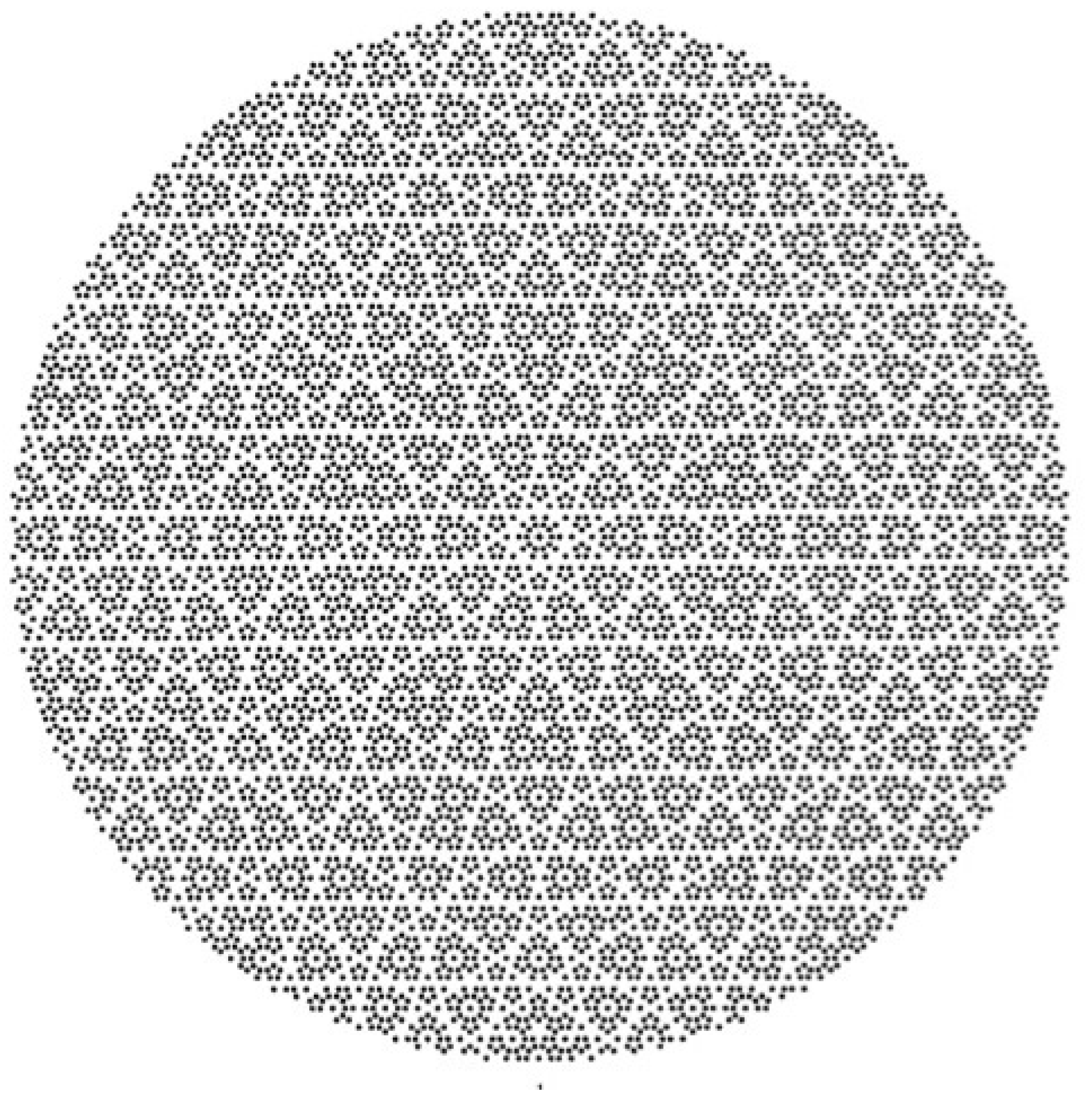
In Figure 12 is shown an example of an observed quasicrystalline surface.

5.10. Algebraic Modeling of Quasicrystals

The identified self-similarity factors, denoted by $\beta$, within quasicrystals exhibit a distinctive mathematical nature known as quadratic Pisot–Vijayaraghavan (PV) numbers. In essence, these numbers correspond to roots greater than 1 of specific quadratic polynomials. These polynomials possess a leading coefficient of 1 and consist of integer coefficients. Notably, the other root of these polynomials is characterized by an absolute value less than 1.

In the case presented above, the factor is the golden mean $\beta =\tau =\frac{1+\sqrt{5}}{2}$. The other ones are

$$\beta ={\tau }^2=\frac{3+\sqrt{5}}{2},\beta =\delta =1+\sqrt{2},\beta =\theta =2+\sqrt{3}.$$

Each value of $\beta$ serves as the defining parameter for a discrete set on the number line, denoted as ${\mathbb{Z}}_{\beta }$ or the set of “beta-integers”, as introduced in [51] (see also [52] and references therein). This set is specifically designed to function analogously to integers within the context of quasicrystalline investigations. A visual representation of this concept is illustrated in Figure 13, depicting the first tau-integers in proximity to the origin.

Beta-lattices are designed to serve as direct substitutes for traditional lattices within the unique framework of quasicrystals. Much like lattices are built upon sets of integers, beta-lattices find their structural basis in beta-integers. This deliberate choice aligns with the goal of seamlessly adapting mathematical structures to the intricate properties of quasicrystals. A typical beta-lattice $\Gamma$ is defined as:

$$\Gamma =\sum _{i=1}^d{\mathbb{Z}}_{\beta }{\mathbf{e}}_i,$$

with $\left({\mathbf{e}}_i\right)$ a base of ${\mathbb{R}}^d$. Examples are shown in Figure 14 and Figure 15.

5.11. Sphere ${\mathbb{S}}^7$ and Octonions (Graves, 1843, Cayley, 1845)

Like $\mathbb{Q},\mathbb{C},\mathbb{H}$, the algebra $\mathbb{O}$ of octonions [53,54] is built by providing the Cartesian product $\mathbb{H}\times \mathbb{H}=\left\{\right(p,q),p,q\in \mathbb{H}\}$ with the commutative addition and the noncommutative and non-associative product:

$$(p,q)+(p^{\prime },q^{\prime })=(p+p^{\prime },q+q^{\prime }),(p,q)(p^{\prime },q^{\prime })=(p{p}^{\prime }-\overline{q^{\prime }}q,q^{\prime }p+q\overline{p^{\prime }}).$$

Let us introduce the eight octonionic basis numbers: $1\equiv (1,0)$ (unity) and

$$\begin{array}{cc}\hfill & \widehat{\mathsf{ı}}\equiv (\widehat{\mathsf{ı}},0),\widehat{\mathsf{ȷ}}\equiv (\widehat{\mathsf{ȷ}},0),\widehat{\mathit{k}}\equiv (\widehat{\mathit{k}},0),\hfill \end{array}$$

(16)

$$\begin{array}{cc}\hfill & \widehat{\mathit{l}}\equiv (0,1),\widehat{\mathsf{ı}}\widehat{\mathit{l}}=(0,\widehat{\mathsf{ı}})\equiv \underline{\widehat{\mathsf{ı}}},\widehat{\mathsf{ȷ}}\widehat{\mathit{l}}=(0,\widehat{\mathsf{ȷ}})\equiv \underline{\widehat{\mathsf{ȷ}}},\widehat{\mathit{k}}\widehat{\mathit{l}}=(0,\widehat{\mathit{k}})\equiv \underline{\widehat{\mathit{k}}},\hfill \end{array}$$

(17)

with the commutation rules

$$\widehat{\mathsf{ı}}\widehat{\mathit{l}}=(0,\widehat{\mathsf{ı}})=-\widehat{\mathit{l}}\widehat{\mathsf{ı}},\widehat{\mathsf{ȷ}}\widehat{\mathit{l}}=(0,\widehat{\mathsf{ȷ}})=-\widehat{\mathit{l}}\widehat{\mathsf{ȷ}},\widehat{\mathit{k}}\widehat{\mathit{l}}=(0,\widehat{\mathit{k}})=-\widehat{\mathit{l}}\widehat{\mathit{k}}.$$

(18)

We then obtain the biquaternion notation for octonions:

$$\mathbb{O}\ni x=p+q\widehat{\mathit{l}}=p_0+p_1\widehat{\mathsf{ı}}+p_2\widehat{\mathsf{ȷ}}+p_3\widehat{\mathit{k}}+q_0\widehat{\mathit{l}}+q_1\underline{\widehat{\mathsf{ı}}}+q_2\underline{\widehat{\mathsf{ȷ}}}+q_3\underline{\widehat{\mathit{k}}}=p+\widehat{\mathit{l}}\overline{q}.$$

(19)

In octonionic calculations we should be aware of the non-associativity of the product, e.g., $(\widehat{\mathsf{ȷ}}\widehat{\mathit{k}})\widehat{\mathit{l}}=\widehat{\mathsf{ı}}\widehat{\mathit{l}}$ whilst $\widehat{\mathsf{ȷ}}(\widehat{\mathit{k}}\widehat{\mathit{l}})=-\widehat{\mathsf{ı}}\widehat{\mathit{l}}$.

The octonionic conjugate of the octonion x is defined as

$$x=(p,q)\mapsto \overline{x}:=(\overline{p},-q).$$

This operation allows defining the Euclidean norm of $x\in \mathbb{O}$ and its inverse if $x\ne 0$.

$$x\overline{x}=\overline{x}x={\left|p\right|}^2+{\left|q\right|}^2\equiv {\left|x\right|}^2,x^{-1}=\frac{\overline{x}}{{\left|x\right|}^2}.$$

Conjugation is involutive: $\overline{x{x}^{\prime }}=\overline{x^{\prime }}\overline{x}$ and one checks that $|x{x}^{\prime }|=|x\left|\right|x^{\prime }|$.

Like the bicomplex notation (10)–(12) for quaternions, we also have the quadricomplex notation for octonions:

$$x=(p,q)=(t,u)+\widehat{\mathsf{ȷ}}(v,w)where\left\{\begin{array}{ccc}t=p_0+p_3\widehat{\mathit{k}}& ,& u=q_0+q_3\widehat{\mathit{k}}\\ v=p_2+p_1\widehat{\mathit{k}}& ,& w=q_2-q_1\widehat{\mathit{k}}\end{array}\right..$$

(20)

The Hurwitz theorem establishes that the real numbers $\mathbb{R}$, complex numbers $\mathbb{C}$, quaternions $\mathbb{H}$, and octonions $\mathbb{O}$ stand as the exclusive normed division algebras over the real numbers, up to isomorphism. Normed in the sense that the product of any two elements satisfies the norm property: $|x{x}^{\prime }|=|x\left|\right|x^{\prime }|$. Moreover, these four algebras represent the sole examples of alternative, finite-dimensional division algebras over the real numbers.

A general rotation in ${\mathbb{R}}^8$, i.e., an element among the 28 elements of SO$\left(8\right)$, can be written through successive right multiplications:

$$\mathbb{O}\ni x\mapsto \left(\left(\left(\left(\left(\left(x{\eta }_1\right){\eta }_2\right){\eta }_3\right){\eta }_4\right){\eta }_5\right){\eta }_6\right){\eta }_7,{\eta }_i\in \mathbb{O},\left|{\eta }_i\right|=1.$$

For a recent review on the role of octonions in Nuclear Physics, see [55].

6. Higher Spheres and Hopf Maps and Fibrations

What about ${\mathbb{S}}^n,n\ge 4$? There is nothing really special from a strictly group point of view when we deal with higher-dimensional spheres. Naturally, many interesting topological features exist, like the Hopf fibrations [56,57].

6.1. Hopf Fibrations

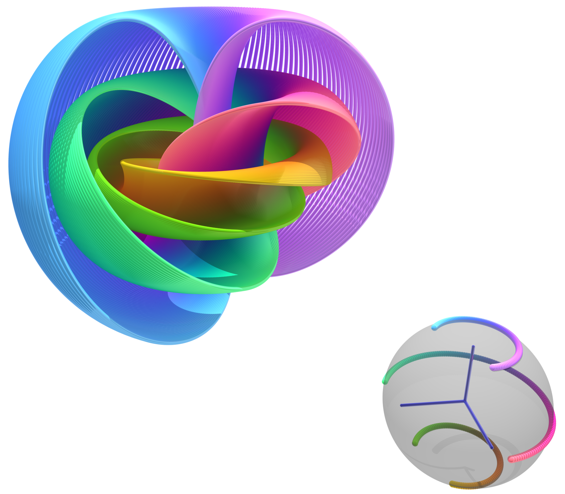
These are the following relations involving spheres, ${\mathbb{S}}^n,n=1,2,3,4,5,7,8,15$:

$${\mathbb{S}}^1\hookrightarrow {\mathbb{S}}^3\stackrel{p}{\to }{\mathbb{S}}^2,{\mathbb{S}}^3\hookrightarrow {\mathbb{S}}^7\stackrel{p}{\to }{\mathbb{S}}^4,{\mathbb{S}}^7\hookrightarrow {\mathbb{S}}^{15}\stackrel{p}{\to }{\mathbb{S}}^8,$$

where “↪” stands for embedding and p is the Hopf map. The first one is displayed in Figure 16.

The Hopf construction, in its broader application, yields circle bundles in the form of ${\mathbb{S}}^{2n+1}\stackrel{p}{\to }\mathbb{C}{\mathbf{P}}^n$ over complex projective space. This construction is essentially a restriction of the topological line bundle over $\mathbb{C}{\mathbf{P}}^n$ to the unit sphere in ${\mathbb{C}}^{n+1}$.

Note the elementary example where one considers ${\mathbb{S}}^1$ embedded in ${\mathbb{R}}^2$ and factoring out by unit real multiplication. One then obtains $\mathbb{R}{\mathbf{P}}^1={\mathbb{S}}^1$. This results in a fiber bundle ${\mathbb{S}}^1\stackrel{p}{\to }{\mathbb{S}}^1$ with the circle ${\mathbb{S}}^0$ as the fiber.

Extending these constructions, one can view ${\mathbb{S}}^{4n-1}$ within quaternionic n-space (${\mathbb{H}}^n$) and factor out by unit quaternion multiplication ($\simeq {\mathbb{S}}^3$) to obtain $\mathbb{H}{\mathbf{P}}^n$. Notably, a bundle ${\mathbb{S}}^7\stackrel{p}{\to }{\mathbb{S}}^4$ with fiber ${\mathbb{S}}^3$ emerges from this construction, connecting quaternionic and real projective spaces.

Similarly, leveraging octonions leads to a bundle ${\mathbb{S}}^{15}\stackrel{p}{\to }{\mathbb{S}}^8$ with fiber ${\mathbb{S}}^7$.

These constructions are often referred to as Hopf bundles, encompassing the realms of real, quaternionic, and octonionic Hopf bundles. Importantly, Adams’ theorem asserts that these bundles represent the exclusive instances of fiber bundles with spheres as the total space, base space, and fiber.

Hopf fibration surfaces show up in the description of quantum entanglement [58,59]. In particle physics they underlie the mathematics of the Dirac monopole. It also appears in general relativity, for instance, in the Robinson congruence (see for instance [60]).

6.2. Group Interpretation of the First Hopf Map: ${\mathbb{S}}^3\stackrel{p}{\to }{\mathbb{S}}^2$

Let us consider the element $\xi =({\xi }_0,{\xi }_1,{\xi }_2,{\xi }_3)$ of ${\mathbb{S}}^3\cong \mathrm{SU}\left(2\right)$ which brings the north pole of ${\mathbb{S}}^2$ to the direction $(x,y,z)\in {\mathbb{S}}^2$:

$$\xi (0,0,0,1)\overline{\xi }=(0,x,y,z),x^2+y^2+z^2=1.$$

This gives the quadratic relations which exemplify the projection p (Hopf’s map) of ${\mathbb{S}}^3$ onto the base space ${\mathbb{S}}^2$:

$${\mathbb{S}}^3\ni \left\{\begin{array}{cc}x=& 2({\xi }_0{\xi }_2+{\xi }_1{\xi }_3)\\ y=& 2({\xi }_2{\xi }_3-{\xi }_0{\xi }_1)\\ z=& {\xi }_0^2+{\xi }_3^2-{\xi }_1^2-{\xi }_2^2\end{array}\right..$$

One easily checks that the Hopf inverse of a point $\in {\mathbb{S}}^2$ is a circle ${\mathbb{S}}^1\subset {\mathbb{S}}^3$ and that the Hopf inverse of a circle ${\mathbb{S}}^1\subset {\mathbb{S}}^2$ is a torus ${\mathbb{S}}^1\times {\mathbb{S}}^1$.

6.3. Group Interpretation of the Second HOPF Map: ${\mathbb{S}}^7\stackrel{p}{\to }{\mathbb{S}}^4$

We here consider the special group isomorphism proper to $B_2\cong C_2$ (see Figure A1):

$$\mathrm{Spin}\left(5\right)\equiv \mathrm{SO}\left(5\right)\times {\mathbb{Z}}_2\simeq G=\left\{g=\left(\begin{array}{cc}a& b\\ c& d\end{array}\right),a,b,c,d\in \mathbb{H},g\overline{{ }^{t}g}={\mathbb{1}}_2\right\}.$$

It is understood through the action of the group G on specific $2\times 2$-quaternionic matrices

$$g\left(\begin{array}{cc}{y}_4& p\\ \overline{p}& -y_4\end{array}\right)\overline{{ }^{t}g}=\left(\begin{array}{cc}{y}_4^{\prime }& p^{\prime }\\ \overline{p^{\prime }}& -y_4^{\prime }\end{array}\right),p\in \mathbb{H},y_4\in \mathbb{R},y_4^2+{\left|p\right|}^2=1.$$

Just consider the group element $g=\left(\begin{array}{cc}a& b\\ -\overline{b_{\alpha }}& \overline{a}\end{array}\right)\in G$, $b_{\alpha }=\overline{a}ba/{\left|a\right|}^2$, which brings the “north pole” of ${\mathbb{S}}^4$, $(y_4=1,p=0)$, to the point $(y_4,p)\in {\mathbb{S}}^4$. We have ${\left|a\right|}^2+{\left|b\right|}^2=1$, i.e., $(a,b)\in {\mathbb{S}}^7$. This gives the quadratic relations:

$$p=-2ba,y_4={\left|a\right|}^2-{\left|b\right|}^2.$$

The Hopf inverse of a point $\in {\mathbb{S}}^4$ is the sphere ${\mathbb{S}}^3\subset {\mathbb{S}}^7$ and the Hopf inverse of a sphere ${\mathbb{S}}^3\subset {\mathbb{S}}^4$ is ${\mathbb{S}}^3\times {\mathbb{S}}^3\simeq \mathrm{SO}\left(4\right)$.

6.4. Group Interpretation of the Third Hopf Map: ${\mathbb{S}}^{15}\stackrel{p}{\to }{\mathbb{S}}^8$

The octonionic Hopf fibration finds its elegant description through the lens of the automorphism group G2 of the normed algebra of octonions. Actually, one can grasp its essence by considering the group Spin$\left(9\right)$ (where Spin$\left(n\right)$ serves as the two-fold covering of SO$\left(n\right)$), as explained in [61].

7. Kepler–Coulomb Problem and Spheres

Concluding our exploration of the world of spheres, it is essential to acknowledge the pivotal role played by ${\mathbb{S}}^1$ and ${\mathbb{S}}^3$, and their complexified versions, in understanding the symmetries of a particle’s motion subjected to the Kepler or Coulomb potential. Alongside the harmonic oscillator, it stands as one of the most emblematic examples of integrable systems within the domain of Galilean classical or quantum mechanics. This symmetry elucidates, at the quantum level, the empirical laws discovered by Balmer in 1885 [62] for describing the spectral line emissions of the hydrogen atom. The literature on this topic is extensive (see, for instance, the review [35]), and its content can attain a high level of mathematical sophistication. To provide some insight, we will first examine in detail the one-dimensional case before sketching the main concepts of the realistic three-dimensional model. It is worth noting that providing a comprehensive account of the symmetries inherent in the Kepler–Coulomb problems, both classically and quantum mechanically, would necessitate delving into a much broader scope of material.

7.1. One-Dimensional Kepler–Coulomb Problem

Consider the energy of a particle of mass m trapped in a well determined on the positive line $q\ge 0$ by the attractive Kepler–Coulomb potential:

$$V\left(q\right)=-\frac{k}{q},k>0,$$

and $V\left(q\right)=\infty$ for $q<0$. Its energy is given by

$$E=\frac{p^2}{2m}-\frac{k}{q}.$$

Regularizing the Kepler problem in the case of negative energy consists in considering the alternative equation:

$$\Theta \stackrel{\mathrm{def}}{=}q(p_0^2+p^2)-2mk=0,q>0.$$

where $p_0=\sqrt{-2mE}$. Let us see how the Balmer laws [62] come to light from the symmetry $A_1$. One considers the three observables defined on the upper half-plane viewed as the phase space $\left\{\right(q,p)\mid q>0,p\in \mathbb{R}\}$:

$$d=qp,{\gamma }_0=\frac{1}{2}q(p^2+p_0^2),{\gamma }_1=\frac{1}{2}q(p^2-p_0^2).$$

Their Poisson brackets $\left(\{f,g\}\stackrel{\mathrm{def}}{=}{\displaystyle \frac{\mathsf{\partial }f}{\mathsf{\partial }q}}{\displaystyle \frac{\mathsf{\partial }g}{\mathsf{\partial }p}}-{\displaystyle \frac{\mathsf{\partial }f}{\mathsf{\partial }p}}{\displaystyle \frac{\mathsf{\partial }g}{\mathsf{\partial }q}}\right)$ obey the commutation relations of the Lie algebra $\mathfrak{sl}(2,\mathbb{R})$ of $\mathrm{SL}(2,\mathbb{R})$:

$$\{d,{\gamma }_0\}={\gamma }_1,\{d,{\gamma }_1\}={\gamma }_0,\{{\gamma }_0,{\gamma }_1\}=p_0^{2}d.$$

After quantization of these classical observables, say $A\mapsto \widehat{A}$, Poisson brackets become commutators, quantum counterparts become (essentially) self-adjoint operators acting in some Hilbert space of quantum states, and a specific unitary irreducible representation of $\mathrm{SL}(2,\mathbb{R})$ is involved, precisely, that one for which the generator $\widehat{{\gamma }_0}$ has nonzero positive integers multiples of $p_0$ as spectral values. This is due to the fact the inverse operator ${\widehat{{\gamma }_0}}^{-1}$ is compact. Remember that an operator A on a infinite-dimensional Hilbert space $\mathcal{H}$ is said to be compact if it can be written in the form $A={\sum }_{n=1}^{\infty }{\lambda }_n\langle {\mathbf{f}}_n,·\rangle {\mathbf{e}}_n$ where $\left\{{\mathbf{e}}_n\right\}$ and $\left\{{\mathbf{f}}_n\right\}$ are orthonormal sets (not necessarily complete) and the ${\lambda }_n$s form a sequence of positive numbers with limit zero (they can accumulate only at zero). Since the classical equation $\Theta =2{\gamma }_0-2mk=0$ becomes $\widehat{\Theta }=2(\widehat{{\gamma }_0}-2mk)\psi =0$, the spectral condition leads directly to the Balmer-like quantization of the energy:

$$n{p}_0-mk=0\iff E=-\frac{m{k}^2}{2n^2}.$$

7.2. Phase Space of the Regularized 1D Kepler–Coulomb Problem: The Complexified Circle with Zero Radius

Let us show that the phase space of the regularized 1D Kepler problem is the complexified circle with zero radius.

Following the Fock method [63,64] for displaying the symmetry of the H-atom, let us introduce the circle variable

$$\xi =\left(\frac{p_0^2-p^2}{p_0^2+p^2},\frac{2p_{0}p}{p_0^2+p^2}\right)\in {\mathbb{S}}^1.$$

(inverse stereographic projection transforming the compactified momentum real line into the unit circle). By imposing that this change of variable be part of a canonical transformation of the phase space, the conjugate variable ${\pi }_{\xi }$ to $\xi$ reads:

$${\pi }_{\xi }=\left(-qp,q\frac{p_0^2-p^2}{2p_0}\right)=\left(-d,\frac{{\gamma }_1}{p_0}\right).$$

One easily checks the two constraints:

$$\left|{\pi }_{\xi }\right|=\frac{mk}{p_0}\mathrm{on} \mathrm{the} \mathrm{energy} \mathrm{shell}\mathrm{and} \xi ·{\pi }_{\xi }=0.$$

Therefore, the pair $\left(\xi ,{\displaystyle \frac{p_0}{mk}}{\pi }_{\xi }\right)$ parametrizes the complex circle in ${\mathbb{C}}^2$ with null radius:

$${\mathbb{S}}_{\mathbb{C}}^1\left(0\right)=\{(z_1,z_2)\in {\mathbb{C}}^2\mid z_1^2+z_2^2=0\}.$$

This is a geometric model for the phase space of the one-dimensional regularized Kepler problem, which can be identified to $T_0^{*}{\mathbb{S}}^1$ (cotangent bundle on ${\mathbb{S}}^1$ with the zero-section deleted, named Moser manifold or Kepler manifold).

7.3. Phase Space of the Three-Dimensional Regularized Kepler–Coulomb Problem

The above material is easily generalizable to three dimensions. Indeed, the phase space of the three-dimensional regularized Kepler problem is the complexification of ${\mathbb{S}}^3$ with radius 0.

Following Fock again in dealing with the more realistic three-dimensional Kepler–Coulomb problem, let us introduce the ${\mathbb{S}}^3$ variable

$$\xi =\left(\frac{p_0^2-{\parallel \mathbf{p}\parallel }^2}{p_0^2+{\parallel \mathbf{p}\parallel }^2},\frac{2p_0\mathbf{p}}{p_0^2+{\parallel \mathbf{p}\parallel }^2}\right)\in {\mathbb{S}}^3.$$

(inverse stereographic projection transforming the 3D-compactified momentum space into a 3-sphere).

By requiring that this change of variable be part of a canonical transformation of the phase space, the conjugate variable ${\pi }_{\xi }$ to $\xi$ together with $\xi$ parametrizes the complexification of ${\mathbb{S}}^3$ in ${\mathbb{C}}^4$ with a null radius. This is the phase space of the three-dimensional regularized Kepler problem, which can be identified with $T_0^{*}{\mathbb{S}}^3$ (cotangent bundle on ${\mathbb{S}}^3$ with the zero-section deleted, Moser manifold or Kepler manifold, as named by Souriau [65]).

The three-dimensional aspect of this structure explains the accidental degeneracy of the discrete spectrum of the hydrogen atom with its SO$\left(4\right)$ symmetry.

8. Conclusions

This contribution is an invitation to embark on an exploration of the realm governed by numbers, symmetries, and intricate symmetry groups, and, as an appealing illustration, to delve into the profound significance encapsulated within the fundamental aspects of the circle and higher-dimensional spheres. Its aim is to share our appreciation for their value in shaping our mathematical comprehension of the natural world and establishing the foundational principles that underpin the laws of physics.