Landau Levels versus Hydrogen Atom

Abstract

The Landau problem and harmonic oscillator in the plane share a Hilbert space that carries the structure of Dirac’s remarkable $so(2,3)$ representation. We show that the orthosymplectic algebra $osp\left(1\right|4)$ is the spectrum generating algebra for the Landau problem and, hence, for the 2D isotropic harmonic oscillator. The 2D harmonic oscillator is in duality with the 2D quantum Coulomb–Kepler systems, with the $osp\left(1\right|4)$ symmetry broken down to the conformal symmetry $so(2,3)$. The even $so(2,3)$ submodule (coined Rac) generated from the ground state of zero angular momentum is identified with the Hilbert space of a 2D hydrogen atom. An odd element of the superalgebra $osp\left(1\right|4)$ creates a pseudo-vacuum with intrinsic angular momentum 1/2 from the vacuum. The odd $so(2,3)$-submodule (coined Di) built upon the pseudo-vacuum is the Hilbert space of a magnetized 2D hydrogen atom: a quantum system of a dyon and an electron. Thus, the Hilbert space of the Landau problem is a direct sum of two massless unitary $so(2,3)$ representations, namely, the Di and Rac singletons introduced by Flato and Fronsdal.

to Richard Kerner,

an inspiring teacher and a devoted friend

who can hear, interpret and transmit the music of the spheres

1. Introduction

Conformal symmetry of Maxwell electrodynamics implies that the Landau problem (magnetostatic) and hydrogen atom problem (electrostatic) enjoy common hidden symmetries. The hydrogen atom is the quantum Coulomb–Kepler problem (Newton potential $1/r$), whereas the Landau problem is the quantum harmonic oscillator (Hooke potential $r^2$), with an additional term accounting for the magnetic field. The duality between the Newton $1/r$ and Hooke $r^2$ potentials can be traced back to Newton’s Principia [1].

The classical Coulomb–Kepler problem in ${\mathbb{R}}^2$ allows for a Moser regularization [2], which maps a bound elliptic orbit to a geodesic on the sphere $S^2$. The time parameter of the cyclic motion is naturally compactified to a circle $S^1$. There is an extension due to Guowu Meng [3] of the Kepler motion from ${\mathbb{R}}^2$ to the future cone of the flat Minkowski space ${\mathbb{R}}^{1,2}$, i.e., $i:\mathit{x}\to (t,\mathit{x})$ such that $t=\left|\mathit{x}\right|$. The Minkowski space ${\mathbb{R}}^{1,2}$ is further mapped by the Cayley transform to its compactification ${\mathcal{M}}^{1,2}=(S^1\times S^2)/{\mathbb{Z}}_2$, which is endowed with a free action of the spectrum generating group $SO(2,3)$ that captures the integrals of Keplerian motion [4,5]. The Coulomb picture is similar in harmony with the fact that electrodynamics in ${\mathbb{R}}^{1,2}$ spacetime possesses the conformal symmetry $SO(2,3)$ [6]. The symplectic group $Sp(4,R)$ is the double-covering of the unit component $S{O}_0(2,3)$ of the anti-de Sitter group $SO(2,3)$ [7]:

$$S{O}_0(2,3)\cong Sp(4,\mathbb{R})/{\mathbb{Z}}_2.$$

By the Newton–Hooke duality, the symplectomorphisms $Sp(4,\mathbb{R})$ of the phase space $T^{*}{\mathbb{R}}^2$ yield a spinorial $SO(2,3)$ representation on the 2D harmonic oscillator [8]. They preserve the constant magnetic field of the underlying planar Landau problem (see our work [5]).

The novelty in the present work is the hidden dynamical symmetry $\mathfrak{so}(2,3)\cong \mathfrak{sp}(4,\mathbb{R})$ of the Hilbert space spanned by the states in all Landau levels, which we denote as $\mathbf{Dirac}$. The Hilbert space $\mathbf{Dirac}$ also associated with the isotropic 2D Harmonic oscillator is a reducible $\mathfrak{so}(2,3)$ module for Dirac’s remarkable representation of the anti-de Sitter (AdS) group $SO(2,3)$ [9]. In other words, $\mathfrak{so}(2,3)$ turns out to be the spectrum generating algebra (SGA) of both the Landau problem and 2D harmonic oscillator. The Bohlin transform incarnates the Newton–Hooke duality [10] between the harmonic oscillator (Landau model) and the quantum Coulomb–Kepler models (with/without magnetic charge):

$$\mathbf{Dirac}:=\mathbf{Di}\oplus \mathbf{Rac}\stackrel{Hooke-Newton}{\leftrightarrow }\left\{2\mathrm{D} \mathrm{charge}-\mathrm{dyon} \mathrm{system}\right\}\oplus \left\{2\mathrm{D} \mathrm{hydrogen} \mathrm{atom}\right\}.$$

The unitary massless conformal $\mathfrak{so}(2,3)$ represenations $D(E_0,s)$ are classified by the minimal conformal energy $E_0$ and the helicity s, with the notations of the seminal work Massless particles, conformal group, and de Sitter universe [11,12]. The conformal energy E turns out to be the eigenvalue of the harmonic oscillator $H_{osc}$, whereas the helicity s is an intrinsic spin that is related to the minimal value of the angular momentum $L_z$ in the plane. Our main result is Theorem 1. It states that the harmonic oscillator Hilbert space $\mathbf{Dirac}$ splits into two $SO(2,3)$ orbits:

(odd)- $\mathbf{Di}=D(1,1/2)$ is the regularized Hilbert space for a quantum system of an electron and a charged magnetic vortex (dyon with helicity $s=\frac{1}{2}$) [10,13];

(even)- $\mathbf{Rac}=D(1/2,0)$ is the regularized Hilbert space for the 2D hydrogen atom quantum Coulomb–Kepler problem described by a massless field with helicity $s=0$, [4,14], reflecting the fact that the group $Sp(4,\mathbb{R})$ is the double-covering of the AdS group $SO(2,3)$.

In our previous work [5], the Landau problem SGA $\mathfrak{so}(2,3)$ emerges from the Jordan algebra $H_2\left(\mathbb{R}\right)$ of real Pauli matrices, or spinorial representation of Minkowski space ${\mathbb{R}}^{1,2}$. Similarly, the spinorial representation of ${\mathbb{R}}^{1,3}$, or the Jordan algebra $H_2\left(\mathbb{C}\right)$ of Pauli matrices, allows us to recover the SGA $\mathfrak{so}(2,4)$ and explain the duality between a 3D hydrogen atom and 4D harmonic oscillator from the (massless) ladder representations of the conformal group $SU(2,2)/{\mathbb{Z}}_2\cong SO(2,4)$ [15,16,17]. The compound quantum system1 of a magnetic monopole (or dyon) and an electric charge, i.e., charge–dyon system is described by a non-zero helicity massless $SU(2,2)$ representation [4,16,19]. By a Majorana reduction from $SU(2,2)$ to $Sp(4,\mathbb{R})$ [20,21], we related the abovementioned 4D and 2D harmonic oscillators.

In this work, we put in the forefront the conformal regularization of the hydrogen atom in ${\mathbb{R}}^D$. Its SGA $\mathfrak{so}(2,D+1)$ acts freely on the compactified Minkowski space ${\mathcal{M}}^{1,D}:=(S^1\times S^D)/{\mathbb{Z}}_2$. The reduction from 3D to 2D yields the planar Landau problem [5].

Here is a short outline of the paper: In Section 1, we define our conventions and recall that the planar Landau problem is a “magnetic deformation” of the 2D harmonic oscillator by adding a topological term to the Hamiltonian. In Section 2, we recall the construction of the Hilbert space $\mathbf{Dirac}$ of Landau level states. By the action of the parity operator, they split into subspaces of odd and even states. In Section 3, we recall the SGA of the hydrogen atom and charge–dyon system in ${\mathbb{R}}^3$. In Section 4, we then revise the Moser regularization in order to reveal the conformal symmetry $SO(2,4)$ of the Coulomb–Kepler system at the classical level. In Section 5, we recall the Hopf fibration $S^3\to S^2$ and relate the geodesic motion on the sphere $S^3$ to a 4D harmonic oscillator. We then use the Majorana reduction from a 4D to a 2D harmonic oscillator. Section 6 is about the Bohlin transform and the Newton–Hooke duality between the 2D Landau problem (potential $r^2$) and the 2D (magnetized) hydrogen atom (potential $1/r$). Section 7 is the original contribution of the paper, which recovers the Dirac’s anti-de Sitter group $SO(2,3)$ [9] acting on the compactified Minkowski space $Sp(2,\mathbb{R})\cong (S^1\times S^2)/{\mathbb{Z}}_2$ as a dynamical group of the Landau problem. Inspired by the seminal work of Ganchev and Palev on parabosonic statistics [22], we bind the odd $\mathbf{Di}$ and even $\mathbf{Rac}$ $\mathfrak{sp}\left(4\right)$ modules into the irreducible $\mathfrak{osp}\left(1\right|4)$ module $\mathbf{Dirac}$ of the spectrum generating orthosymplectic algebra. We conclude by presenting an outlook in Section 8.

2. Planar Landau Problem and 2D Harmonic Oscillator

The classical motion of an electron of mass $\mu$ in an uniform magnetic field is rotation on a circular orbit around a guiding center $\mathit{X}$ with a cyclotron frequency $\omega =\frac{eB}{\mu c}$. In the non-relativistic regime, the minimal coupling of the electron’s charge density to the external magnetic field (as described by the electromagnetic vector potential $\mathcal{A}$) yields the Hamiltonian

$$H=\frac{1}{2\mu }{\left(p-\frac{e}{c}\mathcal{A}\right)}^2.$$

(1)

We choose the symmetric gauge $\mathcal{A}=({\mathcal{A}}_x,{\mathcal{A}}_y)=\frac{B}{2}(-y,x)$ to create a constant uniform magnetic field $\mathit{B}=B\widehat{z}$ along the z-axis. Given its negative charge $e=-\left|e\right|$, the electron is rotating in a positive direction (anti-clockwise) when the magnetic field is positive $B=\left|B\right|$, while for a negative magnetic field $B=-\left|B\right|$, its rotation is in the negative direction.

The gauge-independent kinetic momenta $\mathit{P}$ and the guiding center coordinates $\mathit{X}$ are related to the phase space canonical coordinates $(x,y,p_x,p_y)$ by

$$P_i=\mu {\dot{x}}_i=\mu \frac{\partial H}{\partial p_i}=p_i-\frac{e}{c}{\mathcal{A}}_i,X_i=x_i+\frac{1}{\mu \omega }{ϵ}_{ij}{P}^j.$$

(2)

The coordinates $\mathit{X}=(X,Y)$ are integrals of motion $\dot{X}=0=\dot{Y}$ and decouple from the system (merit of the symmetric gauge). One has two independent Heisenberg algebras $[\mathit{P},\mathit{X}]=0$:

$$[P_x,P_y]=i\frac{\hslash e}{c}B=\frac{i{\hslash }^2}{{\ell }^2},[X,Y]=-i\frac{\hslash }{\mu \omega }=-i{\ell }^2.$$

The Landau Hamiltonian is $H=\frac{{\mathit{P}}^2}{2m}$, and $\mathit{X}$ are the energy zero modes in view of $[H,\mathit{X}]=0$. Here, ℓ stands for the magnetic length ${\ell }^2=\frac{\hslash }{\mu \omega }=\frac{\hslash c}{eB}$. One quantum of magnetic flux ${\mathsf{\Phi }}_0=\frac{hc}{e}$ passes through an area $2\pi {\ell }^2$ in the plane.

Creation and annihilation operators: The kinetic momenta $\mathit{P}=\mathit{p}-\frac{e}{c}\mathcal{A}$ are quantized by the energy creation and annihilation operators $a^{\pm }$. The guiding center coordinates X and Y are integrals of motion, where they are quantized by the magnetic translation operators2 $b^{\pm }$:

$$a^{\pm }=\frac{-P_y\mp i{P}_x}{\sqrt{2\mu \omega \hslash }},b^{\pm }=\frac{X\pm iY}{\ell \sqrt{2}}.$$

(3)

The Hamiltonian H is written with the ladder operators $a^{\pm }$ raising and lowering the energy:

$$H=\frac{\hslash \omega }{2}\{a^{+},a^{-}\},[H,a^{\pm }]=\pm a^{\pm },H|n\rangle =\hslash \omega (n+\frac{1}{2})|n\rangle .$$

(4)

The n-th Landau level is the subspace of states $|n\rangle$ with fixed energy $\hslash \omega (n+\frac{1}{2})$.

The magnetic translations $b^{\pm }$ are “zero modes” of the Hamiltonian H, and $[H,b^{\pm }]=0$ since they commute with the energy shift operators $a^{\pm }$. Therefore, the degeneracy of any Landau level is due to the action of the magnetic translations $b^{\pm }$, i.e., the freedom of choice of the guiding center of the orbit of an electron.

Angular momentum operator:3 $L_z=(x{p}_y-y{p}_x)$ is the generator of the rotational symmetry, where the operators $b^{\pm }$ increase (decrease) the angular momentum eigenvalue:

$$L_z=\frac{\hslash }{2}(b^{+}{b}^{-}-a^{+}{a}^{-}),[L_z,b^{\pm }]=\pm b^{\pm },[L_z,H]=0.$$

(5)

The Landau Hamiltonian H is reduced to an isotropic harmonic oscillator Hamiltonian $H_{osc}$ in two dimensions plus a “magnetic” term proportional to the angular momentum:

$$H=H_{osc}-\mathrm{\Omega }{L}_z=\frac{p_x^2+p_y^2}{2\mu }+\frac{\mu {\mathrm{\Omega }}^2}{2}(x^2+y^2)-\mathrm{\Omega }{L}_z\mathrm{\Omega }=\omega /2.$$

(6)

The Larmour frequency $\mathrm{\Omega }=\frac{eB}{2\mu c}$ is half of the cyclotron frequency $\omega$, i.e., $\mathrm{\Omega }=\frac{\omega }{2}$.

Holomorphic coordinates:4 It is convenient to introduce (anti-)holomorphic coordinates z ($\overline{z}$) on the phase space such that

$$\begin{array}{ccccc}z& =& (x+iy)/2\ell & & \partial =\frac{\partial }{\partial z}=\ell \left(\frac{\partial }{\partial x}-i\frac{\partial }{\partial y}\right)=(p_y+i{p}_x)\ell /\hslash ,\\ \overline{z}& =& (x-iy)/2\ell & & \overline{\partial }=\frac{\partial }{\partial \overline{z}}=\ell \left(\frac{\partial }{\partial x}+i\frac{\partial }{\partial y}\right)=(-p_y+i{p}_x)\ell /\hslash .\end{array}$$

The energy and magnetic translation creation and annihilation operators $a^{\pm }$ and $b^{\pm }$ (see Equation (3)) provide another parametrization of the phase space $T^{*}{\mathbb{R}}^2\cong T^{*}\mathbb{C}$. These are expressed in the holomorphic phase space coordinates as follows:

$$\begin{array}{ccccccc}{a}^{-}& =& \frac{1}{\sqrt{2}}(z+\overline{\partial })& & b^{-}& =& \frac{1}{\sqrt{2}}(\overline{z}+\partial ),\\ a^{+}& =& \frac{1}{\sqrt{2}}(\overline{z}-\partial )& & b^{+}& =& \frac{1}{\sqrt{2}}(z-\overline{\partial }).\end{array}$$

(7)

The Landau Hamiltonian H in the new complex variables reads as follows:

$$H=H_{osc}-\frac{\omega }{2}{L}_z=\frac{\hslash \omega }{2}(z\overline{z}-\partial \overline{\partial })-\frac{\hslash \omega }{2}(z\partial -\overline{z}\overline{\partial })=\frac{\hslash \omega }{2}\{a^{+},a^{-}\}.$$

(8)

The angular momentum is an integral of motion, and thus, $L_z$ commutes with H. It also commutes with the Hamiltonian $H_{osc}$ of the underlying isotropic oscillator:

$$\begin{array}{ccccc}{H}_{osc}& =& \frac{\hslash \omega }{2}(z\overline{z}-\partial \overline{\partial })& =& \frac{\hslash \omega }{4}\left(\{b^{-},b^{+}\}+\{a^{-},a^{+}\}\right).\end{array}$$

It is worth noting that the Hamiltonians H, $H_{osc}$ and $L_z$ can be simultaneously diagonalized. Their common eigenstates form a basis of one Hilbert space, i.e., a Bargmann–Fock space.

3. Landau Levels in a Hilbert Space

The common spectrum of the Landau Hamiltonian H (Equation (1)) and the angular momentum $L_z$ (Equation (5)) is worked out through the standard methods in quantum mechanics:

$$L_z{\psi }_{n,m}=\hslash m{\psi }_{n,m},H{\psi }_{n,m}=\hslash \omega \left(n+\frac{1}{2}\right){\psi }_{n,m},n=n_r+\frac{\left|m\right|-m}{2}.$$

where m is the magnetic quantum number and n is the radial quantum number. The energy spectrum is bounded below, i.e., $n\ge 0$, and the range of the magnetic quantum number m is $m\ge -n$. The radial quantum number $n_r$ is non-negative, i.e., $n_r\ge 0$.

The Landau eigenstates ${\psi }_{m,n}(z,\overline{z})$ have a concise expression when written with the associated Laguerre polynomials:

$${\psi }_{n,m}(z,\overline{z})=C_{n,m}{\left|z\right|}^{\left|m\right|}{L}_{n_r}^{\left|m\right|}{(2|z|}^2)e^{-{\left|z\right|}^2}{e}^{im\phi }n\ge 0m\ge -n.$$

(9)

The scalar product of the eigenfunctions is chosen to be

$$(\psi ,\chi )=\int dx\wedge dy{\psi }^{*}(x,y)\chi (x,y)=4{\ell }^2\int dz\wedge d\overline{z}{\psi }^{*}(z,\overline{z})\chi (z,\overline{z}).$$

The states in all Landau levels are a complete basis of the Hilbert space: 5

$$\mathbf{Dirac}=\underset{n\ge 0}{⨁}{\mathbf{Dirac}}_n=\underset{n\ge 0}{⨁}\underset{m\ge -n}{⨁}{\psi }_{n,m}(z,\overline{z}).$$

(10)

The non-negative integer grading $n\ge 0$ is the Landau level, while the grading in $m\ge -n$ accounts for the angular momentum.

The ground state ${\psi }_{0,0}(z,\overline{z})$ in the lowest Landau level is a Gaussian function with the distribution $|{\psi }_{0,0}{|}^2$ and a standard deviation equal to the magnetic length ℓ:

$${\psi }_{0,0}=\frac{1}{\sqrt{2\pi {\ell }^2}}{e}^{-z\overline{z}}=\frac{1}{\sqrt{2\pi {\ell }^2}}{e}^{-\frac{x^2+y^2}{4{\ell }^2}}.$$

(11)

Any state in the lowest Landau level $n=0$ (LLL) is represented by an arbitrary holomorphic function multiplying the ground state $f\left(z\right)e^{-z\overline{z}}$. The basis of the LLL, or ${\mathbf{Dirac}}_0$, is provided by the holomorphic monomials:

$${\psi }_{0,m}(z,\overline{z})={(m!)}^{-\frac{1}{2}}{\left(b^{+}\right)}^m{\psi }_{0,0}(z,\overline{z})=z^m{e}^{-z\overline{z}}/\sqrt{2^{m}m!2\pi {\ell }^2},$$

since the application of the “zero modes” operators $b^{+}$ do not change the energy level n. The lowest Landau level is a Bargmann space [24]. The higher Landau level ${\mathbf{Dirac}}_n$ is a Bargmann space too, but it is built on the higher vacuum state

$${\psi }_{n,-n}=\frac{1}{\sqrt{2\pi {\ell }^2{2}^{n}n!}}{\overline{z}}^n{e}^{-z\overline{z}}{\mathbf{Dirac}}_n=\underset{m\ge 0}{⨁}\mathbb{C}{\left(b^{+}\right)}^m{\psi }_{n,-n}.$$

The higher vacuum state of the Landau level ${\mathbf{Dirac}}_n$ is created by the vacuum state in the LLL via the n-fold application of the energy creation operator

$${\psi }_{n,-n}={\left(a^{+}\right)}^n{\psi }_{0,0}/\sqrt{n!}.$$

(12)

To summarize: all eigenfunctions in $\mathbf{Dirac}$ can be generated from the ground state by applying the ladder generators $a^{+}$ and $b^{+}$:

$${\psi }_{n,m}(z,\overline{z})=\frac{{\left(a^{+}\right)}^n}{\sqrt{n!}}\frac{{\left(b^{+}\right)}^{n+m}{\psi }_{0,0}}{\sqrt{(n+m)!}}=C_{n,m}{e}^{-{\left|z\right|}^2}\left\{\begin{array}{ccc}\hfill z^m{L}_n^{\left|m\right|}{(2|z|}^2)& & \hfill m\ge 0\\ \hfill {\overline{z}}^{\left|m\right|}{L}_{n+m}^{\left|m\right|}{(2|z|}^2)& & \hfill -n\le m<0\end{array}\right..$$

(13)

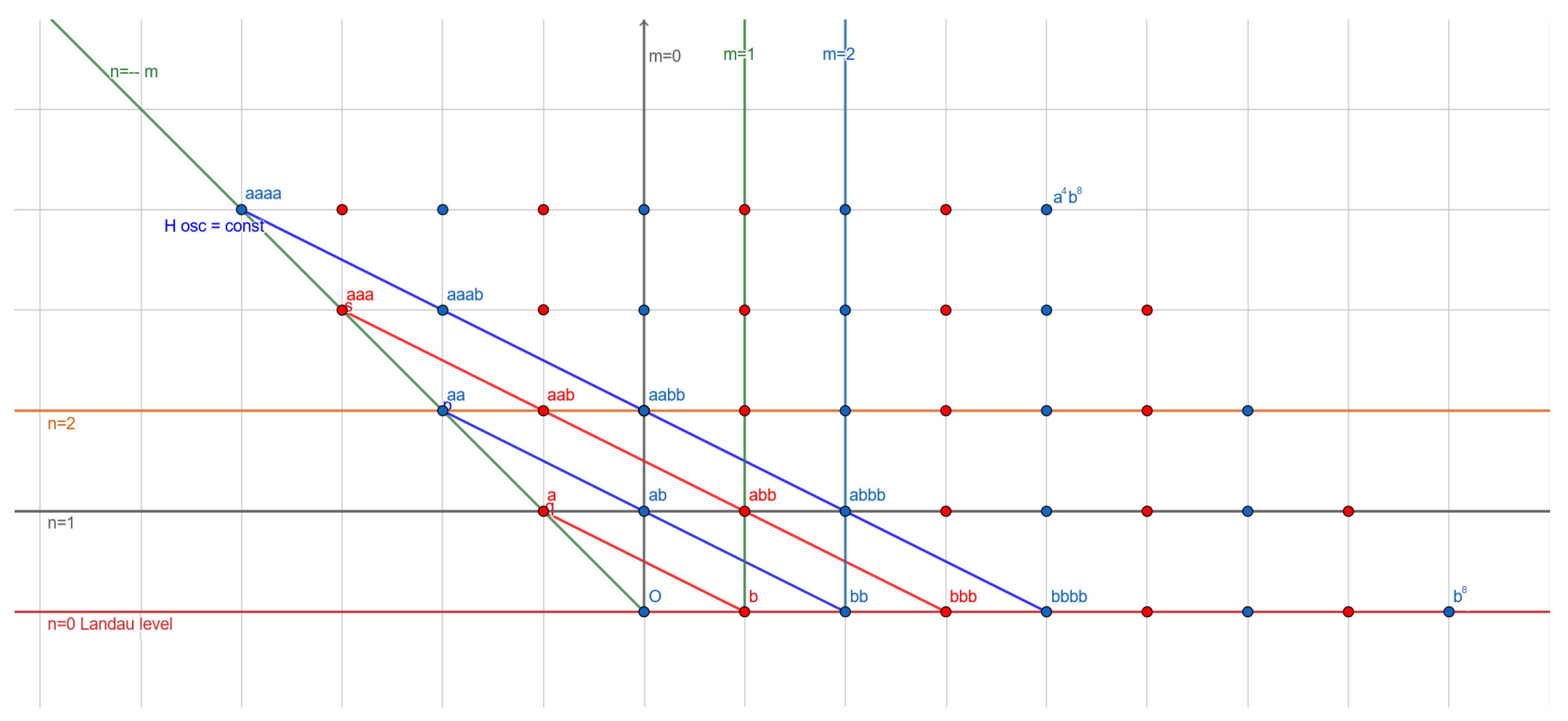
The states ${\psi }_{m,n}(z,\overline{z})$ are in bijection with the integer points on the plane satisfying $n\ge 0$ and $n+m\ge 0$ (see Figure 1). The generators $a^{+}$ and $b^{+}$ correspond to the simple roots of the $B_2$ root system. In Section 8, we relate the orthogonal de Sitter group $SO(2,3)$ to the hidden symmetries of the Landau levels. The construction of a dynamical conformal algebra for the $B_2$ root system was done in a different context in [25].

4. Quantum Coulomb–Kepler System

The electronic orbitals of the non-relativistic hydrogen atom are solutions of the Schrödinger equation with the Hamiltonian

$$H_{atom}=\frac{{\mathit{p}}^2}{2\mu }-\frac{e^2}{r}.$$

Thus, the hydrogen atom is the quantum Coulomb–Kepler system. Here, $\mu$ stands for the reduced mass of the electron–proton system $\mu =m_e{m}_p/(m_e+m_p)$. Due to the great difference in the masses of the electron and the proton $m_p>>m_e$, the reduced mass is very close to the mass of the electron $\mu \approx m_e$; hence, the interpretation is that the electron is propagating in the background electric field created by the proton. The bound states of the hydrogen atom can be built from one ground non-excited state by the spectrum generating group $SO(2,4)$ [26]. These states span the most degenerated representation of $SO(2,4)$, i.e., the massless representation of zero helicity $s=0$ [17]. The other massless $SO(2,4)$ representation of non-zero helicity $s\ne 0$ were interpreted by Barut and collaborators [15,16] as Hilbert spaces for bound states in a system of an electron and dyon. They correspond to MICZ–Kepler systems [27,28] with the Hamiltonian

$$H_{MICZ}=\frac{1}{2\mu }{\left(\mathit{p}-\frac{e}{c}\mathcal{A}\right)}^2-\frac{e^2}{r}+\frac{{\left(eg\right)}^2}{2\mu r^2},\mathcal{A}(x,y,z)=\frac{g}{r(r+z)}(-y,x,0),g=\frac{\hslash cs}{e}.$$

The energy spectrum depends on the principle quantum number $N=n_r+l+\left|s\right|+1$, which is a sum of the radial $n_r$, orbital l quantum numbers and helicity s. The sum implies the accidental degeneracy of the energy levels ($N=\left|s\right|+1,\left|s\right|+2,\dots$):

$$E_N=-\frac{\mu c^2{\alpha }^2}{2N^2}=-\frac{\mu c^2{\alpha }^2}{2(n_r{+l+\left|s\right|+1)}^2},deg\left(E_N\right)=(N+s)(N-s)=\sum _{j=\left|s\right|}^{N-1}(2j+1).$$

The vector potential $\mathcal{A}\left(\mathit{r}\right)$ corresponds to a Dirac monopole with a magnetic charge g. The canonical momenta $\mathbf{\pi }:=\mathit{p}-\frac{e}{c}\mathcal{A}$ do not commute any more due to the magnetic field but satisfy the gauge and rotational invariant commutation relations:

$$[x_i,x_j]=0,[{\pi }_i,x_j]=-i\hslash {\delta }_{ij},[{\pi }_i,{\pi }_j]=is{ϵ}_{ijk}\frac{x_k}{r^3}.$$

(14)

Thus, the MICZ–Kepler system describes an electron propagating in the field of a magnetic monopole also possessing electric charge (dyon). The dyon–dyon system is also reduced to a charge–dyon system [19].

Spectrum generating algebra for 3D hydrogen atom and MICZ–Kepler problem: The conformal algebra $\mathfrak{so}(2,4)$ generators $L_{AB}$ satisfy the commutation relations

$$[L_{AB},L_{CD}]=-i({\eta }_{AC}{L}_{BD}+{\eta }_{BD}{L}_{AC}-{\eta }_{AD}{L}_{BC}-{\eta }_{BC}{L}_{AD})$$

(15)

where the set of indices contains the auxiliary indices $-1$ and 5, in addition to the spacetime indices $\mu =0,1,2,3$:

$$L_{AB}\in \mathfrak{so}(2,4),{\eta }_{AB}=diag(1,1,-1,-1,-1,-1),A,B\in \{-1,0,1,2,3,5\}.$$

The generators of the SGA $\mathfrak{so}(2,4)$ are arranged into an antisymmetric $6\times 6$ matrix:

$$\left(\begin{array}{cccccc}0& L_{-10}& L_{-11}& L_{-12}& L_{-13}& L_{-15}\\ & 0& L_{01}& L_{02}& L_{03}& L_{05}\\ & & 0& L_{12}& L_{13}& L_{15}\\ & & & 0& L_{23}& L_{25}\\ & & & & 0& L_{35}\\ & & & & & 0\end{array}\right)=\left(\begin{array}{cccccc}0& H_{\tau }& M_1& M_2& M_3& D\\ & 0& {\mathrm{\Gamma }}_1& {\mathrm{\Gamma }}_2& {\mathrm{\Gamma }}_3& {\tilde{H}}_{\rho }\\ & & 0& J_3& -J_2& A_1\\ & & & 0& J_1& A_2\\ & & & & 0& A_3\\ & & & & & 0\end{array}\right).$$

(16)

The $\mathfrak{so}(2,4)$ generators of the quantum Kepler and MICZ–Kepler problem read as follows [16]:

$$\begin{array}{cccccccc}\mathit{J}& =& \mathit{r}\times \mathit{\pi }-s\widehat{\mathit{r}}\mathrm{\Gamma }=r\mathit{\pi },\hfill & & D& =\hfill & \mathit{r}·\mathit{\pi }-i,& \\ \mathit{A}& =& \frac{1}{2}\mathit{r}{\pi }^2-\mathit{\pi }(\mathit{r}·\mathit{\pi })+\frac{s}{r}\mathit{J}+\frac{s^2}{2{\mathit{r}}^2}\mathit{r}-\frac{1}{2}\mathit{r},\hfill & & H_{\tau }& =\hfill & \frac{1}{2}\left(r{\pi }^2+\frac{s^2}{r}+r\right),& \\ \mathit{M}& =& \frac{1}{2}\mathit{r}{\pi }^2-\mathit{\pi }(\mathit{r}·\mathit{\pi })+\frac{s}{r}\mathit{J}+\frac{s^2}{2{\mathit{r}}^2}\mathit{r}+\frac{1}{2}\mathit{r},\hfill & & {\tilde{H}}_{\rho }& =\hfill & \frac{1}{2}\left(r{\pi }^2+\frac{s^2}{r}-r\right).\end{array}$$

(17)

The block structure of the matrix induces a rich hierarchy of subalgebras of $\mathfrak{so}(2,4)$. The angular momentum $\mathit{J}$ (with components of the $\mathfrak{so}\left(3\right)$ generators $J_k={\epsilon }_{ijk}{L}_{ij}$) commutes with the radial algebra $\mathfrak{so}(1,2)$ spanned by the dilatation D, $H_{\tau }$ and ${\tilde{H}}_{\rho }$. According to the energy, a different element of the radial algebra is chosen to be the Hamiltonian. For negative energies $E<0$, one diagonalizes the compact Hamiltonian $H_{\tau }$, with the (rescaled) Runge–Lenz vector $\mathit{A}$ as an additional integral of motion (related to the accidental energy degeneracy). Classically, the Runge–Lenz vector points in the direction of the major semi-axis of the elliptical orbit and has a length proportional to the eccentricity of the bound Keplerian orbits. In the quantum Kepler problem, the bound states are transformed into one $SO\left(4\right)$ representation generated by $\mathit{J}$ and $\mathit{A}$ for every eigenvalue of the energy. Similarly, the dual Runge–Lenz vector $\mathit{M}$ is an additional integral of motion for the scattering states and commutes with the non-compact Hamiltonian ${\tilde{H}}_{\rho }$ for positive energies. The scattering eigenstates transform into an $SO(1,3)$ representation generated by $\mathit{J}$ and $\mathit{M}$. The Galilean boost operators $\mathit{r}=\mathit{M}-\mathit{A}$ are related to the symmetries of the lightcone in Minkowski space ${\mathbb{R}}^{1,3}$. The current operator $\mathrm{\Gamma }$, together with $\mathit{J}$, generates another dynamical subgroup $SO(1,3)$, which commutes with the dilatation operator D.

We summarize the subalgebra structure and its relation to the geometry in the

Table 1. 3D Hydrogen atom Spectrum Generating Algebra $\mathfrak{so}(2,4)$ and its subalgebras.

Energy	Hamiltonian	Symmetry	Integrals	Invariant Geometry
$E<0$	$H_{\tau }\in \mathfrak{so}\left(2\right)$	$\mathfrak{so}\left(4\right)$	$\mathit{J},\mathit{A}$	$S^1\times S^3$
$E>0$	${\tilde{H}}_{\rho }\in \mathfrak{so}(1,1)$	$\mathfrak{so}(1,3)$	$\mathit{J},\mathit{M}$	$H^1\times H^3$
$E=0$	$(H_{\tau }+{\tilde{H}}_{\rho })\in \mathbb{R}$	$\mathfrak{so}\left(3\right)+{\mathbb{R}}^3$	$\mathit{J},\mathit{r}$	Lightcone *
	$D\in \mathbb{R}$	$\mathfrak{so}(1,3)$	$\mathit{J},\mathrm{\Gamma }$	$Ad{S}_5$

.

5. Conformal Regularization

Vladimir Fock explained the accidental degeneracy of the energy levels in the hydrogen atom [29] by the presence of hidden symmetries. The essence of Fock’s method is the compactification of the momentum space ${\mathbb{R}}^3$ to a three-dimensional sphere $S^3\subset {\mathbb{R}}^4$. The sphere $S^3$ is invariant under the action of the group $SO\left(4\right)$ generated by the integrals of motion, the angular momentum $\mathit{L}$ and the (rescaled) Runge–Lenz vector $\mathit{A}$.

The Moser regularization [2] for the classical Kepler problem was inspired by Fock’s method. Moser showed that the Kepler bound motion (for negative energies $E<0$) is equivalent to a geodesic motion on a sphere $S^3$ in momentum space. There is a well-forgotten result of Sir Hamilton about the trajectory in the momentum space that he coined a hodograph. Hamilton proved that a hodograph of a Kepler orbit is a circle. We will see that this circle is a great circle on $S^3$.

Moser regularization map [2,4,30]: The stereographic projection maps the 3D sphere $S^3\subset {\mathbb{R}}^4$ to the Euclidean momentum space $\mathit{p}\in {\mathbb{R}}^3$. We have the isomorphism $f:S_N^3\to {\mathbb{R}}^3$ of the chart $S_N^3=S^2-\left\{N\right\}$, where $N=(1,\mathbf{0})$ is the north pole:

$$p_k=\frac{X_k}{1-X_0},X_0=\frac{{\left|\mathit{p}\right|}^2-1}{{\left|\mathit{p}\right|}^2+1},X_k=\frac{2p_k}{{\left|\mathit{p}\right|}^2+1},S^3:X_0^2+{\mathbf{X}}^2=1.$$

(18)

We embed the cotangent bundle $T^{*}{S}^3$ into $T^{*}{\mathbb{R}}^4={\mathbb{R}}^4\oplus {\mathbb{R}}^4$. The additional dimension $X_0$ and the radius of the sphere depend on the energy $E<0$ (here, for simplicity, we consider unit spheres). The conjugate momenta $Y=(Y_0,\mathit{Y})\in {\mathbb{R}}^4$ are defined to be tangent to the sphere $X·Y=X_0{Y}_0+\mathbf{X}·\mathit{Y}=0$. The momenta $\mathit{p}$ are conjugate to the coordinate $\mathit{q}$ in the cotangent bundle $(\mathit{p},\mathit{q})\in T^{*}{\mathbb{R}}^3={\mathbb{R}}^3\oplus {\mathbb{R}}^3$. We extend the stereographic projection (18) to a mapping between the cotangent bundles $T^{*}{\mathbb{R}}^3$ and $T^{*}{S}_N^3$ by

$$\mathit{q}=(1-X_0)\mathit{Y}+Y_0\mathbf{X},Y_0=\mathit{p}·\mathit{q},\mathit{Y}=\frac{1}{2}({\mathit{p}}^2+1)\mathit{q}-(\mathit{p}·\mathit{q})\mathit{p}.$$

(19)

Then, we have a symplectomorphism between $T^{*}{\mathbb{R}}^3$ and $T^{*}{S}_N^3$ since the canonical contact forms $Y·dX=-\mathit{q}·d\mathit{p}$ are related by a canonical transformation.

The geodesic flow on the sphere $S^3$ is given by the Hamiltonian F on $T^{*}{S}^3$:

$$F(X,Y)=\frac{1}{2}{\left|X\right|}^2{\left|Y\right|}^2=\frac{1}{8}{({\mathit{p}}^2+1)}^2{r}^2,r=\left|\mathit{q}\right|,$$

which, under the constraint ${\left|X\right|}^2=1$, yields the free Hamiltonian $\frac{1}{2}{\left|Y\right|}^2$. Hence, the geodesic flow on $S^3$ is symplectically equivalent to the flow of the Kepler Hamiltonian. Suppose we have a new Hamiltonian $J\left(F\right)=\sqrt{2F}-1$; hence, $J^{\prime }\left(F\right)=\frac{1}{\sqrt{2F}}$. The submanifold of $T^{*}{\mathbb{R}}^3$, where $F=\frac{1}{2}$, will be identical to the submanifold $J=0$, where

$$J(\mathit{p},\mathit{q})=\frac{r}{2}({\mathit{p}}^2+1)-1.$$

(20)

To every function, one associates a vector field ${\chi }_f\left(\right)=\omega (f,)$, where $\omega =d\mathit{p}\wedge d\mathit{q}$ is the symplectic form. The Hamiltonian vector fields are related by ${\chi }_J=J^{\prime }\left(F\right){\chi }_F$, and thus, coincide on the submanifold $F=\frac{1}{2}$, which is identical to the submanifold $J=0$. Hence, we have a similarity between the Hamiltonian J and the Kepler Hamiltonian:6

$$J=r\left(H+\frac{1}{2}\right)\mathrm{where}H=\frac{1}{2}{\mathit{p}}^2-\frac{1}{r}.$$

Conformal Hamiltonian: The submanifold $F=\frac{1}{2}$ is then identified as $H=-\frac{1}{2}$ (which would be the energy of the ground state upon quantization7). One has

$$dJ=rd\left(H+\frac{1}{2}\right)\iff {\chi }_J=r{\chi }_H.$$

Let t be the absolute Newtonian time associated with the Kepler Hamiltonian and the vector field ${\chi }_H=\frac{d}{dt}=\{·,H\}$, whereas $\tau$ is the natural parameter along the geodesic flow of ${\chi }_J=\frac{d}{dt}=\{·,J\}$. From the second Kepler’s law about the conservation of the arial velocities, we know that the velocity is bigger when the two bodies are close to each other. The fictitious time $\tau$ is a conformal transformation of the absolute time:

$$\frac{d}{d\tau }=r\frac{d}{dt},\frac{d\tau }{dt}=\frac{1}{r},$$

where it slows down when the two bodies are close, and due to the conformal factor r, the velocity $\frac{d\mathit{x}}{d\tau }$ becomes uniform. The vector field ${\chi }_H$ has a singularity at $r=0$, or $\left|\mathit{p}\right|=\infty$, which is the image of the north pole N on $S^3$. The vector field ${\chi }_J$ is free of singularities; going from t to fictitious time $\tau$ restores N on $S^3$. The collision orbits where we have a clash for a finite time t are regularized so that the clash happens at infinite $\tau$ and the orbit space is compactified. In fact, after quantization, we can set the quantum Kepler Hamiltonian vector field as $H_{atom}=\frac{d}{dt}$ and the quantum conformal Hamiltonian as $H_{\tau }=\frac{d}{d\tau }$.

Hodograph: Without loss of generality, we can rotate the plane of motion to $X_2=0$. The reduced 2D Kepler motion is then equivalent to the motion on the geodesic on $S^2$:

$$X_0=sin\alpha cos\tau ,X_1=sin\tau ,X_3=-cos\alpha cos\tau ,$$

where $\alpha$ is the tilt of the great circle of $S^2$. The eccentricity of the orbit is identified with $ϵ=sin\alpha$ and it is proportional to the magnitude $\left|\mathit{A}\right|$ of the Runge–Lenz vector. The tangent to the sphere momenta is found by differentiation with respect to the evolution parameter $\tau$:

$$Y_0=-sin\alpha sin\tau ,Y_1=cos\tau ,Y_3=cos\alpha sin\tau .$$

With the help of the cotangent extension of the stereographic projection $T^{*}{S}_N^3\to T^{*}{\mathbb{R}}^3$ and Equations (18) and (19), we obtain the trajectory in the phase space:

$$\begin{array}{ccccccccc}{p}_1& =& \frac{sin\tau }{1-ϵcos\tau },& & p_3& =& -\frac{\sqrt{1-{ϵ}^2}cos\tau }{1-ϵcos\tau },p_2& =& 0,\\ q_1& =& cos\tau -ϵ,& & q_3& =& \sqrt{1-{ϵ}^2}sin\tau ,q_2& =& 0.\end{array}$$

This geodesic line is the hodograph; it is a great circle with a center depending on the eccentricity $ϵ$:

$$p_1^2+{(p_3-tan\alpha )}^2=1+{tan}^2\alpha ,tan\alpha =\frac{ϵ}{\sqrt{1-{ϵ}^2}}.$$

Mapping one hodograph to another one in the plane is a conformal transformation $SO(2,3)$. This hodograph will be mapped under the Newton–Hooke duality to the planar cyclotronic motion of an electron in a constant magnetic field.

6. Newton–Hooke Duality

The Moser regularization is a symplectic isomorphism between the Kepler motion and the free geodesic motion on the sphere $S^3$. Furthermore, the geodesic motion on $S^3$ is equivalent to the motion of a harmonic oscillator in ${\mathbb{R}}^4$ by the Kustaanheimo–Stiefel transform [31]. It allows the quantum Coulomb–Kepler problem (hydrogen atom) and the quantum MICZ–Kepler problem to be mapped to a 4D harmonic oscillator [32]. We are referring to this correspondence as the Newton–Hooke duality.

Compactified Minkowski space: The flat Minkowski space ${\mathbb{R}}^{1,3}$ with metric ${\eta }_{\mu \nu }=diag(+1,-1,-1,-1)$ can be written as a spinor:

$$\tilde{x}=x^{\mu }{\sigma }_{\mu }=\left(\begin{array}{cc}{x}^0+x^3& x^1+i{x}^2\\ x^1-i{x}^2& x^0-x^3\end{array}\right)\in H_2\left(\mathbb{C}\right),{\left(\mathit{x}\right)}^2=det\tilde{x}={\eta }_{\mu \nu }{x}^{\mu }{x}^{\nu }.$$

The Kepler orbits are conic sections and they appear as an intersection of the light cone $det\tilde{x}=0$ with some plane. The Cayley transform C is a map that sends a Hermitian matrix to a unitary one:

$$C:H_2\left(\mathbb{C}\right)\to U\left(2\right),U=\frac{1-i\tilde{x}}{1+i\tilde{x}}.$$

The Cayley transform is a Lorenzian counterpart of the stereographic projection. It compactifies both space and time:

$$C:{\mathbb{R}}^{1,3}\to {\mathcal{M}}^{1,3}:=U\left(2\right)=U\left(1\right)\times SU\left(2\right)/{\mathbb{Z}}_2\cong S^1\times S^3/{\mathbb{Z}}_2.$$

We define the space of the unitary matrices U to be the compactified Minkowski space. On the space ${\mathcal{M}}^{1,3}$, we have an action of the conformal group $SU(2,2)$ by fractional linear transformations:

$$U\to gU:=\frac{AU+B}{CU+D},g=\left(\begin{array}{cc}A& B\\ C& D\end{array}\right)\in SU(2,2).$$

The compactified Minkowski space ${\mathcal{M}}^{1,3}$ is a homogeneous space of the conformal group $SU(2,2)$. The group $SU(2,2)$ is the double-covering of $S{O}_0(2,4)$, the identity component of the conformal group $SO(2,4)$. There is a manifestly covariant description of the compactified Minkowski space ${\mathcal{M}}_{1,3}$ as a projective quadric in ${\mathbb{R}}^{2,4}$, the Klein–Dirac quadric:8

$${\mathcal{M}}^{1,3}=Q/{\mathbb{R}}^{*},Q=\{{\eta }_{AB}{y}^A{y}^B=0\},{\eta }_{AB}=diag(+1,+1,-1,-1,-1,-1).$$

KS transform and Hopf fibration: The regularized Kepler orbits live on the cotangent bundle $T^{*}{S}^3$ to the sphere $S^3$ with the zero section removed [4]:

$$T^{+}{S}^3=T^{*}{S}^3-\left\{0_{sec}\right\}.$$

Definition 1.

The Kustaanheimo–Stiefel ($KS$) transform is the map

$$KS:T^{+}{S}^3\to T^{+}{S}^2\subset {\left({\mathbb{R}}^{*}\right)}^4\times {\mathbb{R}}^4\to {\left({\mathbb{R}}^{*}\right)}^3\times {\mathbb{R}}^3$$

where the 4D harmonic oscillator phase space coordinates $(u,w)\in {\left({\mathbb{R}}^{*}\right)}^4\times {\mathbb{R}}^4$ are related to the 3D Kepler phase space $(\mathit{q},\mathit{p})\in {\left({\mathbb{R}}^{*}\right)}^3\times {\mathbb{R}}^3$ coordinates through the Hopf fibration map extended with the derived momentum relations (${\left|\mathit{z}\right|}^2=u_1^2+u_2^2+u_3^2+u_4^2$):

$$\begin{array}{ccc}{q}_1& =& u_1{u}_3+u_2{u}_4,\\ q_2& =& u_2{u}_3-u_1{u}_4,\\ q_3& =& -u_1^2-u_2^2+u_3^2+u_4^2,\end{array}\begin{array}{ccc}{p}_1& =& -(u_1{w}_3+w_1{u}_3+u_2{w}_4+w_2{u}_4)/{\left|\mathit{z}\right|}^2,\\ p_2& =& -(u_2{w}_3+w_2{u}_3-w_1{u}_4-u_1{w}_4)/{\left|\mathit{z}\right|}^2,\\ p_3& =& (u_1{w}_1+u_2{w}_2-u_3{w}_3-u_4{w}_4)/{\left|\mathit{z}\right|}^2.\end{array}$$

(21)

The coordinates on $T^{+}{S}^3$ are subject to the constraint

$$K=u_1{w}_2-u_2{w}_1+u_3{w}_4-u_4{w}_3=2\lambda .$$

The Hopf fibration represents a 3D vector $\mathit{x}\in {\mathbb{R}}^3$ as a “square root” of a spinor $\mathit{Z}\in {\mathbb{C}}^2$ in view of

$$\left|\mathit{q}\right|={\left|\mathit{Z}\right|}^2,\mathit{Z}=\left(\begin{array}{c}{u}_1+i{u}_2\\ u_3+i{u}_4\end{array}\right),{\left|\mathit{Z}\right|}^2={\mathit{Z}}^{†}\mathit{Z}.$$

(22)

The KS transformation can be seen as a phase space extension of the Hopf fibration

$$0\to S^1\hookrightarrow S^3\to S^2\to 0,$$

where the kernel consists of the spinors $e^{i\theta }\mathit{z}\in S^1$. The new Hamiltonian $J\left(F\right)$ (20) can be written in terms of spinorial variables as a Hamiltonian of a 4D harmonic oscillator:

$$J(\mathit{Z},\mathit{W})=\frac{1}{2}{\left|\mathit{Z}\right|}^2+\frac{1}{2}{\left|\mathit{W}\right|}^2-1,KS:J(\mathit{Z},\mathit{W})\to J(\mathit{p},\mathit{q}).$$

Its image under the KS transform yields the Hamiltonian $J(\mathit{p},\mathit{q})$, which is equivalent to the Kepler Hamiltonian H. The 4D harmonic oscillator modes are components of a Dirac spinor that transforms under the conformal group $SU(2,2)$, thus giving a spinorial $SO(2,4)$ representation in view of the isomorphism $SU(2,2)/{\mathbb{Z}}_2\cong SO(2,4)$.

Majorana reduction from 4D to 2D: The 4D Dirac $SU(2,2)$ spinor is reduced by a Majorana projection to a 4D real spinor that is transformed under $Sp(4,\mathbb{R})$ (see our companion paper [5]). The reduction of the KS transform to the Bohlin (Levi–Civita) transform is done by the Majorana reduction:

$$u_2=u_4=0,w_2=w_4=0,$$

which amounts to taking a square root of a vector in the 2D plane $q_1=\eta$ and $q_3=\xi$. The Bohlin transform stems from the change to parabolic coordinates $u_1$ and $u_3$ in the complex plane:

$$\xi +i\eta =z^2,\begin{array}{ccccc}\xi & =& u_1^2-u_3^2,& & p_{\xi }=(u_1{w}_1-w_3{u}_3)/{\left|z\right|}^2,\\ \eta & =& 2u_1{u}_3,& & p_{\eta }=-(u_1{w}_3+w_1{u}_3)/{\left|z\right|}^2,\end{array}$$

(23)

where the real spinor $\psi =\left(\begin{array}{c}{u}_1\\ u_3\end{array}\right)$ is written with one complex number $z=u_1+i{u}_3$. The Levi–Civita mapping is then a sympletic extension of the the trivial Hopf fibration:

$$0\to S^0\hookrightarrow S^1\to S^1\to 0,$$

where the dimension zero sphere $S^0={\mathbb{Z}}_2$ is in the kernel, thus reflecting the fact that any pair of parabolic coordinates $(u_1,u_3)$ and $(-u_1,-u_3)$ parametrize one point $\xi +i\eta \in \mathbb{C}$.

A 4D real Majorana spinor is equivalent to a 2D Weyl spinor. We now use a conformal regularization of the 2D quantum Coulomb–Kepler system (with or without magnetic charge). These reduced systems are embedded into a 2D harmonic oscillator via a Bohlin (Levi–Civita) transform [10].

7. Planar Harmonic Oscillator and Newton–Hooke Duality

The harmonic oscillator $H_{osc}$ and Landau Hamiltonian H have a common basis of states ${\psi }_{m,n}(z,\overline{z})$, which are also eigenvalues of the angular momentum $L_z$:

$$H_{osc}=\frac{\hslash \omega }{2}\left(a^{+}{a}^{-}+b^{+}{b}^{-}+2\right),H=\hslash \omega \left(a^{+}{a}^{-}+\frac{1}{2}\right)=H_{osc}-\mathrm{\Omega }{L}_z.$$

The spectrum of the harmonic oscillator Hamiltonian is easy to calculate:

$$H_{osc}{\psi }_{n,m}(z,\overline{z})=\hslash \omega \left(N+\frac{1}{2}\right){\psi }_{n,m}(z,\overline{z})N=n+\frac{m}{2}=n_r+\frac{\left|m\right|}{2}.$$

We distinguish two types of $H_{osc}$ eigenspaces, with N as an integer (blue) or half-integer (red). The parity operator depends on the parity of the angular momentum eigenvalue m:

$$\mathrm{\Pi }{\psi }_{n,m}(z,\overline{z})={\psi }_{n,m}(e^{i\pi }z,e^{-i\pi }\overline{z})={(-1)}^m{\psi }_{n,m}(z,\overline{z}).$$

The Hamiltonian $H_{osc}$ has a finite degeneracy $2N+1$, contrary to the infinite degeneracy of the Landau levels, i.e., the eigenspaces of H.

Duality between a harmonic oscillator and H-atom or charge–vortex system: The duality between oscillators in various dimensions and hydrogen atom or charge–dyon (charged vortex) were thoroughly studied in the works of the Armenian Mathematical Physics school (for a pedagogical review and extensive literature, see [13,33]). From the perspective of two-time physics, the same dualities were studied by Itzhak Bars and collaborators (see [34] and references therein).

The 2D isotropic harmonic oscillator with Hamiltonian $H_{osc}$ is in duality with the 2D hydrogen atom. The duality is provided by the Levi–Civita regulatization or Bohlin transform. It is a two-sheeted covering the complex mapping

$$w=z^2\mathrm{where}z=\left|z\right|e^{i\phi }w=r{e}^{i\theta }$$

which induces the mapping between $\phi \in [0,2\pi )$ and $\theta \in [0,4\pi )$, where $\theta$ winds twice for one period of $\phi$:

$$r=z\overline{z},\theta =2\phi .$$

The angular momentum operator $L_z=-i\hslash \frac{\partial }{\partial \phi }$ with integer eigenvalues $m\in \mathbb{Z}$ (reflecting the single valuedness of the wavefunction) transforms into a rotation operator in the new angle $\theta$; hence, the $J_z$ eigenvalues j run on half-integer values:

$$L_z=-i\hslash \frac{\partial }{\partial \phi },2J_z=2\times \left(-i\hslash \frac{\partial }{\partial \theta }\right),m=2j=2(l+s).$$

Here, the angular momentum is the sum of the “orbital” angular momentum $l\in \mathbb{Z}$ and the intrinsic angular momentum (helicity) $s\in \frac{1}{2}\mathbb{Z}$. The Schrödinger equation for $H_{osc}$ in z variables induces another Schrödinger equation in w (or for $r,\theta$) for the quantum Coulomb–Kepler system, with or without a magnetic charge. The wavefunction of the oscillator with energy levels $N=n_r+\left|j\right|$ are mapped to the eigenfunctions of the (magnetized) 2D hydrogen atom with finitely degenerated energy levels ($N=\left|s\right|,\left|s\right|+1,\dots$):

$$E_N=-\frac{\mu c^2{\alpha }^2}{2{(N+\frac{1}{2})}^2}=-\frac{\mu c^2{\alpha }^2}{2(n_r+|l+s|+\frac{1}{2}{)}^2},deg\left(E_N\right)=2(N-|s\left|\right)+1.$$

Here, $\alpha =e^2/\hslash c$ is the fine structure constant. These wavefunctions depend on $\theta$ and live on a two-sheeted Riemann surface $w=z^2$, with a double-covering of the z-complex plane:

$${\psi }_{n,m}(r,\theta )=C_{N,j}^{\left(s\right)}{e}^{-\beta r}{\left(\beta r\right)}^{\left|j\right|}{L}_{N-\left|j\right|}^{2\left|j\right|}\left(2\beta r\right)e^{ij\theta }\beta =1/\left(N+1/2\right).$$

These are $4\pi$-periodic ${\psi }_{n,m}(r,\theta +4\pi )={\psi }_{n,m}(r,\theta )$ since the wavefunction is single-valued. However, the $2\pi$-translation of $\theta$ yields the parity operator (red and blue dots in Figure 1):

$$\mathrm{\Pi }{\psi }_{n,m}(r,\theta )={\psi }_{n,m}(r,\theta +2\pi )={(-1)}^{2j}{\psi }_{n,m}(r,\theta )={(-1)}^m{\psi }_{n,m}(r,\theta ),$$

where for odd m, we have a $(-1)$ (blue states) eigenvalue, while for even m, we have $(+1)$ (red states). We introduce a $U\left(1\right)$ factor, taking care of the boundary conditions in view of ${(-1)}^{2s}={(-1)}^m$, and we end up with a $2\pi$-periodic and single-valued function ${\tilde{\psi }}_{n,m}(r,\theta )$:

$${\psi }_{n,m}(r,\theta )=e^{is\theta }{\tilde{\psi }}_{n,m}(r,\theta ),{\tilde{\psi }}_{n,m}(r,\theta +2\pi )={\tilde{\psi }}_{n,m}(r,\theta ).$$

The effective Hamiltonian acting on ${\tilde{\psi }}_{m,n}(r,\theta )$ defines a 2D charge–vortex system [13,35]:

$$H_{flux}=\frac{1}{2\mu }{\left(\mathit{p}-\frac{e}{c}\mathcal{A}\right)}^2-\frac{e^2}{r},\mathcal{A}(x,y)=\frac{g}{r^2}(-y,x),g=\hslash cs/e.$$

The number $2s$ counts the elementary fluxes $hc/e$ in the flux of the magnetic field $\mathit{B}\left(\mathit{r}\right)$. The Dirac quantization condition $eg/\hslash c\in \frac{1}{2}\mathbb{Z}$ guarantees that ${\tilde{\psi }}_{n,m}(r,\theta )$ is single-valued. When $s=0$, we recover the 2D hydrogen atom with no magnetic field. For $s=\frac{1}{2}$, one has a localized magnetic flux at the origin $r=0$. An ideal infinite solenoid transversal to the plane creates a magnetic vortex carrying a magnetic charge g:

$$\mathit{B}\left(\mathit{r}\right)=rot\mathcal{A}\left(\mathit{r}\right)=2\pi g\delta \left(\mathit{r}\right).$$

The limit of the 3D MICZ–Kepler problem when the flux g is increasing proportional to the area surface yields the Landau problem with a constant transversal field B in the symmetric gauge as a planar limit:

$$\mathcal{A}=\underset{g\to \infty }{lim}\underset{r\to \infty }{lim}\frac{g}{r(r+z)}(-y,x,0)=\frac{B}{2}(-y,x,0)\mathrm{provided}B=\frac{2g}{r^2}=const.$$

8. Dirac’s Remarkable Representation

The action of the spectrum generating algebra allows for creating all the states in a Hilbert space starting from one (or several) ground state(s). What is the dynamic algebra of the Hilbert space $\mathbf{Dirac}$ of the Landau levels? In other words, can we endow the Hilbert space of the Landau problem $\mathbf{Dirac}$ (Equation (10)) with a structure of a representation of an algebra such that its action generates all the states from some lowest (energy) weight vector(s)?

The phase space $T^{*}{\mathbb{R}}^2$ coordinates on the 2D plane are $\{p_x,p_y,x,y\}$. The magnetic field is encoded into the symplectic form of the phase space throughout the commutation relations. Therefore, the group $Sp(4,\mathbb{R})$ of symplectomorphisms is a natural symmetry for the Landau problem. On the other hand, the symplectic group $Sp(4,\mathbb{R})$ is the double-covering of a de Sitter group:

$$S{O}_0(2,3)\cong Sp(4,\mathbb{R})/{\mathbb{Z}}_2,\mathfrak{so}(2,3)\cong \mathfrak{sp}(4,\mathbb{R}).$$

The conformal group $SO(2,3)$ is the maximal symmetry of the Maxwell equations in the flat Minkowski space ${\mathbb{R}}^{1,2}$. We then expect to see the conformal algebra $\mathfrak{so}(2,3)\cong \mathfrak{sp}(4,\mathbb{R})$ as a dynamical symmetry of the Landau problem, as well as the 2D hydrogen atom.

Klein–Dirac quadric: Dirac came out with a spinorial realization of $\mathfrak{so}(2,3)$ in his seminal paper A Remarkable Representation of the 3 + 2 de Sitter Group [9]. The de Sitter group $SO(2,3)$ has a homogeneous space $d{S}_4$ defined by the Klein–Dirac quadric in five-dimensional flat ambient space with coordinates $y^A$:

$$y_{-1}^2+y_0^2-y_1^2-y_2^2-y_3^2=R^2={\eta }_{ab}{y}^a{y}^b,{\eta }_{ab}=diag(+1,+1,-1,-1,-1).$$

The de Sitter group $SO(2,3)$ is the conformal group of the Minkowski space ${\mathbb{R}}^{1,2}$; it acts freely on the compactified Minkowski space of rays in $y\in {\mathbb{R}}^{2,3}$:

$${\mathcal{M}}^{1,2}=(S^1\times S^2)/{\mathbb{Z}}_2.$$

The flat Minkowski space ${\mathbb{R}}^{1,2}$ is isometric to the space real Hermitian matrices $S\in H_2\left(\mathbb{R}\right)$, and the metric is given by det. The symplectic Cayley transform C maps the real symmetric matrix $S=S^T$ to the real symplectic matrix [36]:

$$C:H_2\left(\mathbb{R}\right)\to Sp(2,\mathbb{R}),C\left(S\right)=M:=\frac{11-\mathcal{J}S}{11+\mathcal{J}S},\mathcal{J}=\left(\begin{array}{cc}0& 1\\ -1& 0\end{array}\right).$$

Hence, it compactifies the flat Minkowski space ${\mathbb{R}}^{1,2}$ to the compactified Minkowski space:

$$C:{\mathbb{R}}^{1,2}\to {\mathcal{M}}^{1,2}:=Sp(2,\mathbb{R})\cong (S^1\times S^2)/{\mathbb{Z}}_2.$$

The space ${\mathcal{M}}^{1,2}$ is a homogeneous space for the fractional linear action of the double-covering $Sp(4,\mathbb{R})$ of the identity component of the conformal group $S{O}_0(2,3)$:

$$M\to gM:=\frac{AM+B}{CM+D},g=\left(\begin{array}{cc}A& B\\ C& D\end{array}\right)\in Sp(4,\mathbb{R}).$$

The reduction of the Minkowski space ${\mathbb{R}}^{1,3}\cong H_2\left(\mathbb{C}\right)$ to ${\mathbb{R}}^{1,2}\cong H_2\left(\mathbb{R}\right)$ induces the Majorana reduction of an $SU(2,2)$ spinor to an $Sp(4,\mathbb{R})$-spinor (see [5] for more details).

It was shown that the Dirac remarkable representation is spanned by the quadratic polynomials of the modes of 2D isotropic harmonic oscillator [8].

Lemma 1.

The skewsymmetric generators $m_{ab}=-m_{ba}$, $a,b\in \{-1,0,1,2,3\}$ quadratic in the oscillators modes $a^{\pm }$ and $b^{\pm }$

$$\begin{array}{cccccc}\hfill m_{12}& =& \frac{1}{2}(z\partial -\overline{z}\overline{\partial })& =& \frac{1}{4}\left(\{b^{-},b^{+}\}-\{a^{-},a^{+}\}\right)& ,\\ \hfill m_{23}& =& \frac{1}{4}(z^2+{\overline{z}}^2-{\partial }^2-{\overline{\partial }}^2)& =& \frac{1}{4}\left(\{a^{-},b^{+}\}+\{a^{+},b^{-}\}\right)& ,\\ \hfill m_{31}& =& \frac{i}{4}(z^2-{\overline{z}}^2+{\partial }^2-{\overline{\partial }}^2)& =& \frac{i}{4}\left(\{a^{-},b^{+}\}-\{a^{+},b^{-}\}\right)& ,\\ \hfill m_{1-1}& =& \frac{1}{4i}(z^2-{\overline{z}}^2-{\partial }^2+{\overline{\partial }}^2)& =& \frac{i}{4}\left(a^{+2}-a^{-2}+b^{-2}-b^{+2}\right)& ,\\ \hfill m_{2-1}& =& \frac{1}{4}(z^2+{\overline{z}}^2+{\partial }^2+{\overline{\partial }}^2)& =& \frac{1}{4}\left(a^{-2}+a^{+2}+b^{-2}+b^{+2}\right)& ,\\ \hfill m_{3-1}& =& -\frac{i}{2}\left(z\partial +\overline{z}\overline{\partial }-1\right)& =& -\frac{i}{4}\left(\{a^{-},b^{-}\}-\{a^{+},b^{+}\}\right)& ,\\ \hfill m_{01}& =& -\frac{1}{2}\left(z\overline{\partial }-\overline{z}\partial \right)& =& -\frac{1}{4}\left(a^{-2}+a^{+2}-b^{-2}-b^{+2}\right)& ,\\ \hfill m_{02}& =& -\frac{i}{2}\left(\overline{z}\partial +z\overline{\partial }\right)& =& -\frac{i}{4}\left(a^{-2}-a^{+2}+b^{-2}-b^{+2}\right)& ,\\ \hfill m_{03}& =& \frac{1}{2}\left(z\overline{z}+\partial \overline{\partial }\right)& =& -\frac{1}{4}\left(\{a^{+},b^{+}\}+\{a^{-},b^{-}\}\right)& ,\\ \hfill m_{-10}& =& \frac{1}{2}\left(z\overline{z}-\partial \overline{\partial }\right)& =& \frac{1}{4}\left(\{a^{-},a^{+}\}+\{b^{-},b^{+}\}\right)& ,\end{array}$$

(24)

satisfy the commutation relation

$$[m_{ab},m_{cd}]=0,[m_{ab},m_{bc}]=-i{\eta }_{bb}{m}_{ac},{\eta }_{ab}=diag(+1,+1,-1,-1,-1).$$

Therefore the generators $m_{ab}$ provide a representation of the conformal algebra $\mathfrak{so}(2,3)$. The latter representation is identified with the Dirac remarkable representation of $\mathfrak{so}(2,3)\cong \mathfrak{sp}(4,\mathbb{R})$.

Proof. 

By straightforward calculation. One can also give a conceptual proof by Majorana reduction of a spinor from $\mathfrak{su}(2,2)$ to $\mathfrak{sp}(4,\mathbb{R})$. For details, see [5]. □

Subalgebras of the conformal algebra $\mathfrak{so}(2,3)$: the isotropic rays in the five-dimensional space ${\mathbb{R}}^{2,3}$ carry a linear representation of the conformal group $SO(2,3)$ with generators

$$m_{ab}=\left(\begin{array}{ccccc}0& m_{-10}& m_{-11}& m_{-12}& m_{-13}\\ & 0& m_{01}& m_{02}& m_{03}\\ & & 0& m_{12}& m_{13}\\ & & & 0& m_{23}\\ & & & & 0\end{array}\right)=\left(\begin{array}{ccccc}0& h_{\tau }& M_1& M_2& D\\ & 0& {\mathrm{\Gamma }}_1& {\mathrm{\Gamma }}_2& {\tilde{h}}_{\rho }\\ & & 0& l_3& A_1\\ & & & 0& A_2\\ & & & & 0\end{array}\right).$$

The conformal Hamiltonian. The operator $h_{\tau }$ generates the flow on the compactified time variable $\tau$ running on the circle $S^1$; it coincides with the (normalized) harmonic oscillator Hamiltonian $H_{osc}=\hslash \omega h_{\tau }$. The conformal Hamiltonian $h_{\tau }\in \mathfrak{so}\left(2\right)$ commutes with $l_i=\frac{1}{2}{ϵ}_{ijk}{m}_{jk}$ in the $\mathfrak{so}\left(3\right)$ subalgebra and generates the flows on the compactified Minkowski space:

$$[h_{\tau },l_i]=0,\mathfrak{so}{\left(2\right)}_{h_{\tau }}\oplus \mathfrak{so}\left(3\right)\subset \mathfrak{so}(2,3),{\mathcal{M}}_{1,2}=(S^1\times S^2)/{\mathbb{Z}}_2.$$

Runge–Lenz vector and $\mathfrak{so}\left(3\right)$ subalgebra: The generators $\{l_3,A_1,A_2\}$ close the $\mathfrak{so}\left(3\right)$ algebra:

$$[A_1,A_2]=i{l}_3,[l_3,A_1]=i{A}_2,[l_3,A_2]=-i{A}_1.$$

Only $l_3=L_z/\hslash$ has a meaning of geometric rotation. $\mathit{A}$ is a two-dimensional vector $(A_1,A_2)$ [14,37]; it plays the role of Runge–Lenz generators for the 2D Kepler problem.

Dual Runge–Lenz vector. The generators $\{l_3,M_1,M_2\}$ close a copy of the subalgebra $\mathfrak{so}(1,2)$. The $\mathfrak{so}(1,2)$ generators are the integrals of motion for the non-compact generator ${\tilde{h}}_{\rho }$. The generator ${\tilde{h}}_{\rho }$ is a Hamiltonian for the scattering states when the energy is positive $E>0$ and $\rho$ is the non-compact time parameter. Thus, the 2D vector $(M_1,M_2)$ is the analog of the dual Runge–Lenz vector generation flow on a 2D hyperboloid.

Galilean boost and rotations: The Hamiltonian $h_{free}=h_{\tau }+{\tilde{h}}_{\rho }$ is related to the parabolic motion of zero energy $E=0$. Its integrals of motion span the Euclidean subalgebra $\mathfrak{so}\left(2\right)⋉{\mathbb{R}}^2$: the semidirect sum of pure rotations and Galilean boosts $\mathit{r}=\mathit{M}-\mathit{A}$.

We summarize the subalgebras of the reduced SGA $\mathfrak{so}(2,3)\cong \mathfrak{sp}(4,\mathbb{R})$ in a

Table 2. 2D Hydrogen atom Spectrum Generating Algebra $\mathfrak{so}(2,3)$ and its subalgebras.

Energy	Hamiltonian	Symmetry	Integrals	Inv. Geometry
$E<0$	$h_{\tau }\in \mathfrak{so}\left(2\right)$	$\mathfrak{so}\left(3\right)$	$L_3,\mathit{A}$	$S^1\times S^2$
$E>0$	${\tilde{h}}_{\rho }\in \mathfrak{so}(1,1)$	$\mathfrak{so}(1,2)$	$L_3,\mathit{M}$	$H^1\times H^2$
$E=0$	$(h_{\tau }+{\tilde{h}}_{\rho })\in \mathbb{R}$	$\mathfrak{so}\left(2\right)+{\mathbb{R}}^2$	$L_3,\mathit{r}$	Lightcone *
	$D\in \mathbb{R}$	$\mathfrak{so}(1,2)$	$L_3,\mathrm{\Gamma }$	$Ad{S}_4$

.

Radial algebra $\mathfrak{so}(1,2)$: The operators $h_{\tau }$, ${\tilde{h}}_{\rho }$ and D span the radial subalgebra $\mathfrak{so}(1,2)$. It originates in the conformal transformations of the time variable [35]. The radial algebra $\mathfrak{so}(1,2)$ is the commutant of the spatial rotation algebra $\mathfrak{so}{\left(2\right)}_{l_3}$ generated by $l_3$:

$$\mathfrak{so}(1,2)\oplus \mathfrak{so}{\left(2\right)}_{l_3}\subset \mathfrak{so}(2,3).$$

The non-compact generators ${\tilde{h}}_{\rho }$ and D can be combined into raising and lowering operators of the compact conformal energy operator $h_{\tau }$:

$$c^{\pm }=-{\tilde{h}}_{\rho }\pm iD=a^{\pm }{b}^{\pm },[c^{+},c^{-}]=-2h_{\tau },[h_{\tau },c^{\pm }]=\pm c^{\pm }.$$

The operators $c^{\pm }=a^{\pm }{b}^{\pm }$ shift the quantum number n by one unit without affecting m:

$$c^{\pm }{\psi }_{n,m}=N_{mn}{\psi }_{n\pm 1,m},h_{\tau }{\psi }_{n,m}=\left(N+\frac{1}{2}\right){\psi }_{n,m},l_3{\psi }_{n,m}=m{\psi }_{n,m}.$$

The commutation $[l_3,c^{\pm }]=0$ allows for the separation of variables in the Schrödinger equation.

Lemma 2.

The Hilbert space $\mathbf{Dirac}$ of the Landau levels (and the 2D isotropic harmonic oscillator) is a reducible $\mathfrak{so}(2,3)$ representation with generators $m_{ab}$. All the states ${\psi }_{n,m}(z,\overline{z})$ in the Landau levels space (10) are generated by the $\mathfrak{so}(2,3)$ action from the two lowest Landau level states:

$${\psi }_{0,0}\in \mathbf{Rac}=D(1/2,0)and{\psi }_{0,1}=b^{+}{\psi }_{0,0}\in \mathbf{Di}=D(1,1/2).$$

Proof. 

The $\mathfrak{so}(2,3)$ module $\mathbf{Dirac}$ is the Hilbert space for the 2D isotropic harmonic oscillator with the conformal Hamiltonian $H_{osc}=\hslash \omega h_{\tau }$, as well as the Landau level space with a Landau Hamiltonian $H=H_{osc}-\frac{\omega }{2}{L}_z$. The unitary $\mathfrak{so}(2,3)$ modules with positive energy are denoted as $D(E_0,s)$ [12], where $E_0$ is the minimal energy of the conformal Hamiltonian $h_{\tau }$ and s is the minimal value of the angular momentum $l_3$.

Half of the states in $\mathbf{Dirac}$ (Equation (10)) can be obtained by the action of $\mathfrak{so}(2,3)$ on the ground state ${\psi }_{0,0}\in \mathbf{Rac}=D(1/2,0)$. These are the states with even eigenvalues $n+\frac{m}{2}$ of the conformal energy $H_{osc}$. The odd eigenvalues are obtained by acting on the “odd” ground state $b^{+}{\psi }_{0,0}\in \mathbf{Di}=D(1,1/2)$. □

Theorem 1.

The superalgebra $\mathfrak{osp}\left(1\right|4)$ is an SGA for the Landau levels space $\mathbf{Dirac}$. It generates all the Landau level states from one ground state:

$$\mathbf{Dirac}\cong \mathfrak{osp}\left(1\right|4){\psi }_{0,0}.$$

Proof. 

The super algebra generated by the creation and annihilation operators $a^{\pm }$ and $b^{\pm }$ is the orthosymplectic superalgebra $B(0,2):=\mathfrak{osp}\left(1\right|4)$:

$$\mathfrak{osp}\left(1\right|4)=\mathfrak{sp}\left(4\right)⋉(\mathbb{C}{a}^{\pm }\oplus \mathbb{C}{b}^{\pm }).$$

Its even subalgebra is $\mathfrak{sp}\left(4\right)$; it is the algebra closed by the quadratic polynomials in the parabosonic generators $a^{\pm }$ and $b^{\pm }$. Ganchev and Palev [22] showed that n barabososonic generators span the orthosymplectic algebra $B(0,n)=\mathfrak{osp}\left(1\right|2n)$. From this perspective, the SGA of the Landau levels space is the superalgebra of two parabosonic generators, namely, $a^{\pm }$ and $b^{\pm }$. □

Remark 1.

Super-extensions of the Landau problem based on motions on a supergroup manifold are known (see [38] and the reference therein); however, in our approach, the supersymmetry arises as a dynamical symmetry of the standard “bosonic” planar Landau problem.

The Landau levels Hilbert space $\mathbf{Dirac}$ is a $OSp\left(1\right|4)$ module with a natural splitting into two $SO(2,3)$ orbits, namely, odd states $\mathbf{Di}$ (charge–vortex system [10,13]) and even states $\mathbf{Rac}$ (2D hydrogen atom [20]):

$$\mathbf{Dirac}=\mathbf{Di}\oplus \mathbf{Rac}=SO(2,3){\psi }_{0,1}\oplus SO(2,3){\psi }_{0,0}=OSp\left(1\right|4){\psi }_{0,0}.$$

9. Outlook and Perspectives

In this paper, we examined the Moser conformal regularizations of the classical Coulomb–Kepler problem for bound motions in 2D and 3D. The Kepler orbits are naturally lifted to the compactified Minkowski space endowed with a free linear action of the conformal group. The quantum Coulomb–Kepler problems (i.e., the hydrogen atoms in 2D and 3D) yield upon regularization the Newton–Hooke dual oscillator models, which are the harmonic oscillators in 2D and 4D, respectively. The Cayley transform and Hopf fibration are instrumental in obtaining the massless ladder $U(2,2)$-representations. The Majorana reduction of the ladder $U(2,2)$-representations lead to the Dirac’s remarkable representation of the anti-de Sitter group $SO(2,3)$ on the Hilbert space $\mathbf{Dirac}$ of the planar Landau model and 2D harmonic oscillator.

Table 3. The big picture of the reduction of the harmonic oscillators into Kepler problems.

Coulomb–Kepler Model	Harmonic Oscillator	MICZ–Kepler Model
3D hydrogen atom	4D oscillator	3D charge–dyon
Massless $SO(2,4)$ rep	$SU(2,2)$ rep	Massless $SO(2,4)$ rep
	Landau model on $S^2\subset {\mathbb{R}}^3$
Helicity $s=0$	Planar 2D Landau model	Helicity $s=\frac{1}{2}$
Even module	$OSp\left(1\right|4)$ rep $\mathbf{Dirac}$	Odd module
2D hydrogen atom	2D oscillator	2D charge–dyon(vortex)
$SO(2,3)$ rep $\mathbf{Rac}$	$Sp(4,\mathbb{R})$ rep $\mathbf{Di}\oplus \mathbf{Rac}$	$SO(2,3)$ rep $\mathbf{Di}$

summarize the interrelation between the oscillators and Kepler models in our text.

A parity operator distinguishes between odd and even states in the Landau levels, splitting the Hilbert space into two irreducible unitary massless $\mathfrak{so}(2,3)$ representations. We show that the Newton–Hooke duality maps the even (odd) subspace of the Landau problem $\mathbf{Dirac}$ onto the Hilbert space of the 2D hydrogen atom $\mathbf{Rac}$ (charge–vortex system $\mathbf{Di}$). The unitary $\mathfrak{so}(2,3)$ representations $\mathbf{Di}$ and $\mathbf{Rac}$ are then identified as the odd and even states in one orthosymplectic $\mathfrak{osp}\left(1\right|4)$ module. This module is the same as the Fock space for two parabosons subject to the parastatistics quantization of H.S. Green [39]. We can speculate that under some conditions, the $\mathfrak{osp}\left(1\right|4)$ supersymmetry is broken down to the underlying conformal $\mathfrak{so}(2,3)$ symmetry, and a different physical Hilbert space is realized according to the magnetic charge of the vacuum state. A reformulation of the Landau levels $OSp\left(1\right|4)$ supersymmetry in terms of chiral superfields along the lines of [40,41] is desirable. Another direction is explore the connection between the coherent states of the orthosymplectic algebra $\mathfrak{osp}\left(1\right|4)$ developed in [42] and the eigenstatesstates in the Landau levels.

The reduction from a 4D to a 2D harmonic oscillator yields the planar Landau problem [5]. By analogy, the Newton–Hooke dual 3D magnetized hydrogen atom can be seen as a higher-dimensional Landau model [43,44] of an electron in the background with a Dirac magnetic monopole. Landau models and their Newton–Hooke duals can also be thought of as a toy model for quantum systems with a confinement. It would be natural to explore the Landau problems in higher dimensions [45,46] as the dual models of the quantum (magnetized) Kepler problems [47,48] attached to other Euclidean Jordan algebras [3]. Long ago Barut and Kleinert proposed a relativistic framework based on $SO(2,4)$ symmetry that incorporates the discrete mass spectrum and the internal degeneracies of hadron states [49]. These ideas indicate a possible track to attack the confinement in quantum chromodynamics [50,51].

It will be interesting to understand the relation between matrix models for the Landau models, Jordan algebra modules and noncommutative matrix geometry studied by Michel Dubois-Violette, Richard Kerner and John Madore [52].