Abstract
We consider the decay of the inflaton in Starobinsky-like models arising from either an theory of gravity or no-scale supergravity models. If Standard Model matter is simply introduced to the theory, the inflaton (which appears when the theory is conformally transformed into the Einstein frame) couples to matter predominantly in Standard Model Higgs kinetic terms. This will typically lead to a reheating temperature of ∼3 × GeV. However, if the Standard Model Higgs is conformally coupled to curvature, the decay rate may be suppressed and vanishes for conformal coupling . Nevertheless, the inflaton decays through the conformal anomaly, leading to a reheating temperature of the order of GeV. The Starobinsky potential may also arise in no-scale supergravity. In this case, the inflaton decays if there is a direct coupling of the inflaton to matter in the superpotential or to gauge fields through the gauge kinetic function. We also discuss the relation between the theories and demonstrate the correspondence between the no-scale models and the conformally coupled theory (with ).
1. Introduction
A key aspect of the difference between the ‘old’ model of inflation, based on a first-order phase transition [1,2,3], and the ‘new’ inflationary Universe [4,5] is the ability to recover from the era of exponential expansion, or a graceful exit from inflation [6,7,8,9,10,11,12]. In old inflation, bubble percolation was incompatible with resolving the cosmological problems tackled by inflation. In new inflation (and in all subsequent ‘newer’ inflationary models), a graceful exit is a built-in feature. Indeed, a graceful exit is possible regardless of whether inflation takes place at small field values rolling toward large field values (hilltop inflation) or at large field values rolling to the origin in field space (plateau models). The evolution of the field driving inflation, inflaton (the name for this field was first used in [13], when it was coined by Dimitri Nanopoulos when asked what this field was if we divorce its identity from the SU(5) Higgs adjoint, which was the commonly assumed candidate for the field driving inflation), is governed by its equation of motion and begins with a period of slow roll characterized by exponential expansion, , where a is the cosmological scale factor and is a nearly constant Hubble parameter during inflation. Slow roll naturally ends with an oscillatory phase, where the inflaton oscillates about a minimum and a matter-dominated phase, , begins.
However, at some point, inflaton oscillations must give way to a radiation-dominated Universe. This transition is most easily accomplished through the decay of the inflaton [13,14,15], leading to a period of reheating. Provided that the inflaton decay products scatter and thermalize [16,17,18,19,20,21,22,23,24,25], the standard radiation-dominated era of the early Universe is produced. In this review, dedicated to the accomplishments of Professor Dimitri Nanopoulos, we revisit the possibilities for inflaton decay in Starobinsky-like models and explore these same models when derived from no-scale supergravity [26,27].
The Starobinsky model [28] predates the original models of inflation based on a GUT phase transition and was an attempt to find a solution for a singularity-free Universe. The model is based on an theory of gravity, which is conformally equivalent to a theory that combines Einstein gravity with a scalar field, potentially serving as the inflaton [29,30]. Furthermore, the first calculation of a nearly flat scale-independent density fluctuation spectrum was performed in this context [31,32].
Shortly after the advent of the new inflationary model, it was recognized that supersymmetry may play an important role [33,34,35,36] in preventing an inflationary hierarchy problem, which requires the inflaton mass to be ≪, where GeV is the reduced Planck mass. Supergravity is the extension of supersymmetry that incorporates gravitational interactions, and it is natural to construct inflationary models consistent with supergravity. However, minimal supergravity models are plagued with the so-called problem [37,38], in which scalars tend to obtain large (Hubble scale) masses, preventing an extended period of inflation. This problem is alleviated [39] in no-scale supergravity models [26,27], formulated on a maximally symmetric field-space manifold, and have been derived as the effective low-energy theory from string theory [40,41,42,43]. Of particular interest here is the class of inflationary models based on no-scale supergravity, which yields a model related to the Starobinsky model [44,45,46].
In this contribution, we will focus on inflaton decay in Starobinsky-like models and related models based on no-scale supergravity. Some of these results may also be applicable to T-model attractors [47]. We begin by reviewing the Starobinsky model, augmented with a matter sector that, for simplicity, consists only of the Standard Model Higgs boson (or the supersymmetric Higgs, as the case may be). We also consider the possibility that the Higgs boson is coupled to curvature (with a coupling ), where the decay rate of the inflaton vanishes when . In this case, the dominant decay mechanism comes from the coupling to through the conformal anomaly [48]. We also consider Starobinsky-like models derived in no-scale supergravity and examine the prospects for decay in these models. In general, inflaton decays in no-scale models are highly suppressed [49,50]. In the absence of a direct (superpotential) coupling of the inflaton to the Standard Model, decay to gauge bosons through the gauge kinetic function may be the dominant channel for inflaton decay. For a review on building inflationary models in no-scale supergravity, see Ref. [51].
In what follows, we begin with the Starobinsky model as a model of inflation and compare the inflationary observables—the tilt in the perturbation spectrum and the tensor-to-scalar ratio—to CMB results. We consider several possibilities for coupling the Standard Model to the theory and calculate the inflaton decay rate. Even in the Einstein frame, fields are generally not canonically normalized, and we discuss the procedure for determining canonical field coordinates. We also discuss inflaton decay through the conformal anomaly. In Section 3, we discuss the derivation of a Starobinsky-like model in the context of no-scale supergravity. We also review the possibilities for inflaton decay in this context. Also in this case, fields are generally non-canonical, and we briefly review the transformation to canonical field coordinates. Finally, in Section 4, we relate the formulations of the inflationary model in the contexts of gravity and no-scale supergravity. There is a close correspondence between the two when the Higgs is conformally coupled with . Our conclusions are presented in Section 5.
2. The Starobinsky Model and Inflaton Decays
The Starobinsky model of inflation [28] can be formulated by adding an term to the conventional linear Einstein–Hilbert action:
where is a constant. Here, we work in units where . Upon introducing a Lagrange multiplier , this action may be rewritten in the form
Then, following the conformal transformation [29,30,52,53]
we can rewrite the action in the Einstein frame as
Note the appearance of an additional scalar degree of freedom, with a non-canonical kinetic term and potential . By making a field redefinition, , Equation (4) may be written as
When , the potential is now seen with the well-known form of the Starobinsky potential,
This potential is shown in Figure 1.
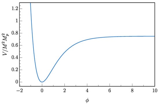
Figure 1.
The scalar potential (6) in the Starobinsky model of inflation [28].
As an inflationary model, the potential (6) leads to observables in excellent agreement with observations by Planck and other CMB experiments [54,55,56,57]. The comparison to experiments is easily made by first computing the slow-roll parameters, and for single-field inflationary models,
where the prime denotes a derivative with respect to inflaton field . Of particular interest is the tilt in the spectrum of scalar perturbations, [54,55], where
and the tensor-to-scalar ratio, r [56], where
The overall inflationary scale, M, is set by the amplitude of scalar perturbations, [54,55],
The number of e-folds, , of inflation between the initial and final values of the inflaton field is given by the formula
The number of e-folds between when the pivot scale () exits the horizon and the end of inflation is denoted by . Inflation ends when and . Typical values of are in the range ∼ 50–60, depending on the mechanism that ends inflation [54,55,58,59].
For the Starobinsky model, it is straightforward to compute the inflationary observable listed above [44]:
For the Starobinsky potential, [60,61] and for . In this case, we find , , and .
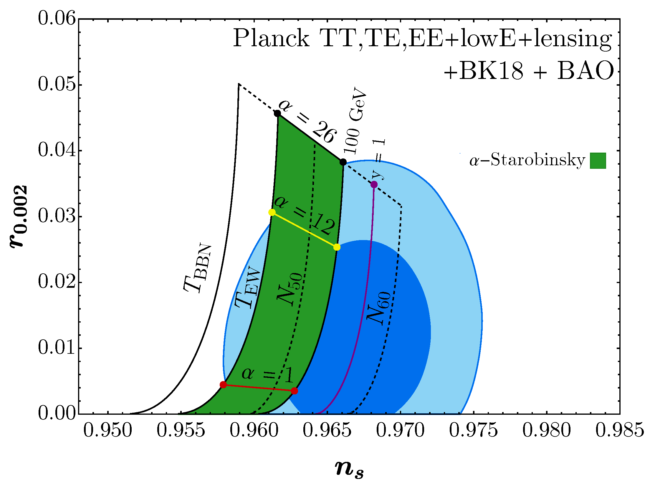
We show in Figure 2, taken from Ref. [61], the 68% and 95% CL regions of the plane allowed by the Planck and Keck/BICEP2 data [54,55,56]. The (nearly) horizontal line (labeled ; where the parameter refers to a generalization of the Starobinsky model whereby the exponent in Equation (6) becomes [45,62,63]) corresponds to the predictions of the Starobinsky model (6) for to e-folds, corresponding to limits from reheating (see below) 100 GeV GeV, with the latter corresponding to the upper limit on from the limit on gravitino production and the relic density of a 100 GeV lightest supersymmetric particle. The other nearly vertical curves correspond to (from left to right) MeV (solid); (dotted); GeV, obtained when a perturbative decay coupling is (with ) (solid); and (dotted). For the -Starobinsky model [45,62,63], we shade the region in green, which respects the constraint and the relic density constraint of GeV. For more details, see [61].
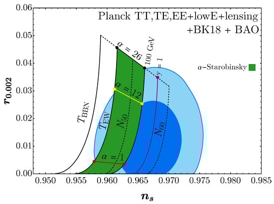
Figure 2.
Plot of the CMB observables and r. The blue shadings correspond to the 68% and 95% confidence level regions from Planck data combined with BICEP2/Keck results [54,55,56]. The red dots show the predictions of the -Starobinsky potential with (i.e., the Starobinsky model) for (left) and (right) corresponding to limits from reheating 100 GeV GeV. The upper pair of yellow (black) dots are the predictions when (the largest value of consistent with 68% CL (95% CL) CMB observations and GeV). The vertical lines correspond to the prediction assuming a reheating temperature (or value of as appropriate) of MeV, GeV, , GeV, GeV, and .
As described above, the -Starobinsky model will inflate and produce density fluctuation in agreement with the experiment. When , the inflaton begins a period of oscillations, and the energy density in these oscillations scales as , typical of a matter-dominated Universe. These oscillations continue until inflaton decays occur sufficiently fast to produce radiation. How this occurs depends on how the Standard Model is introduced in the context of inflationary theory and how the inflaton couples to the Standard Model (SM).
We first consider a simple model by adding a complex scalar field H to the action:
After performing the same conformal transformation (3) and the field redefinition , the above action can be rewritten as
By expanding the second line around the minimum, , we obtain a canonical kinetic term for the complex scalar, , as well as the couplings of the inflaton to H:
The dominant contribution to the decay, , comes from the first term (the second term gives a contribution which is suppressed by the Higgs mass), and the rate is given by
where is the number of the real scalar degrees of freedom of the SM Higgs doublet.
It is often useful to perform a field redefinition to obtain canonical fields in a particular background by using Riemann normal coordinates (RNCs). The term can be eliminated, and the coupling of the inflaton to Higgs is purely a potential interaction. The RNC fields can be obtained quite generally. Let us consider a Lagrangian of the form
where is a symmetric metric and is the potential. Here, we use the Latin indices for the flavor eigenbasis. To compute the interactions around the minimum, we introduce the field expansion , where is the vacuum expectation value and is the field fluctuation. Following the discussions in [64,65,66], the symmetrized covariant derivatives of the potential can be expressed as
where the covariant derivatives are symmetrized and include all permutations multiplied by a factor of symmetry . Here, we take the derivatives with respect to field , evaluated at their VEV . The Christoffel symbols are given by
By using these definitions, we find that the canonically normalized mass matrix at the minimum is given by . To canonically normalize the fields and transform from the flavor to mass eigenbasis, we introduce a tetrad that flattens the metric:
where the lowercase letters correspond to the mass eigenbasis and the indices may be raised or lower by using the Kronecker delta: or . The inverse tetrad can be computed by using the expression .
In Riemann normal coordinates, there are no cubic derivative interactions, which significantly simplifies the computation. Thus, in this case, the cubic interaction can arise only from the potential terms. From action (16), we find that the field metric of the kinetic terms can be expressed as
where . At the minimum, the VEVs of these fields are . We find that the tetrad at the minimum is given by
Finally, we compute the three-particle scattering amplitude by using Equation (20), which includes a symmetry factor for two identical final states in the amplitude. To compute the scattering amplitude in the mass eigenbasis, we use
and find
These couplings lead to the decay rate (18). For more details on how to use the RNCs to compute the scattering amplitudes, see Refs. [64,65,66].
Another alternative description of the model entails a conformal transform into the conformal frame where all the scalar fields conformally couple to gravity. This is achieved by the conformal transformation
with the inflaton () and the conformal factor satisfying
Then, the above action can be rewritten as [67]
In this frame, the scalar fields are canonical and conformally coupled to gravity without any kinetic mixing, and the decay is induced by the cubic interaction from the potential. Focusing on the Standard Model Higgs with , the decay is predominantly induced by the last term in Equation (29), and we recover the decay rate given in Equation (18), which is expected due to frame independence.
One may also introduce a non-minimal coupling to gravity, :
The conformal transformation in this case is
In the Einstein frame, this is equivalent to
where now .
To compute the decay rate in this frame, one can again expand the couplings around the minimum, which gives rise to the following dominant trilinear couplings:
The rate is then (see also [68,69] for discussions on inflaton decay in these models)
Alternatively, we may move to the conformal frame by
with the inflaton () and the conformal factor satisfying
and we obtain [67]
This form of action makes it manifest that the interaction between the inflaton and the Higgs is controlled by the combination . The decay is again induced by the cubic interaction from the last term in the potential (even if we assume that the Higgs mass is of the order of the electroweak scale after integrating out the inflaton, the inflaton coupling to the Higgs induces an additional Higgs mass term above the inflaton mass scale [70]; however, as long as is small, the generated mass is suppressed compared with M; therefore, it has a negligible contribution to the decay rate), and not surprisingly, the rate is given by Equation (34). Note that a very large negative value for forces the Higgs to participate in the inflationary dynamics, making it the so-called Higgs- inflation model [71,72,73,74]. In this case, the (p)reheating dynamics can be non-perturbative [75,76,77,78], and we do not consider this regime in the following.
The above formula shows that if the Higgs conformally couples to gravity, with , the inflaton does not decay into the Higgs. In this case, the inflaton predominantly decays into Standard Model gauge bosons through the trace anomaly [48]. In general, the coupling between the inflaton and Standard Model particles in the Starobinsky model is expressed to the lowest order as
where is the trace of the stress–energy tensor. One can see that Equations (17) and (33) indeed take this form. If the matter sector is (classically) conformal, and assuming the absence of direct coupling between the gauge sector and gravity beyond the minimal one in the original frame, is predominantly sourced by the trace anomaly. The origin of the trace anomaly depends on the regularization scheme (although the final result itself does not) [79,80,81]. For instance, in dimensional regularization, the inflaton couples to the gauge bosons as , with spacetime dimension , after the conformal transformation. This factor of is compensated by the pole arising from the wavefunction renormalization (and self-interactions in the non-Abelian case), resulting in a finite term in the limit proportional to , where is the beta function counting both heavy and light degrees of freedom. In addition, the inflaton directly couples to heavy degrees of freedom through their mass terms. After integrating out heavy degrees of freedom, the contribution from the mass term cancels with the one from the wavefunction renormalization, leaving only light degrees of freedom, as demonstrated in [79,80,81]. As a result, the trace anomaly is given by
where i runs over all the different gauge groups, a runs over the generators of each gauge group, and is the fine structure constant of gauge group i. The beta function is given by
where counts only the number of light degrees of freedom as explained above, and for U(1) (note that this corresponds to the beta function for ), for SU(2), and for SU(3) for the Standard Model (the Minimal Supersymmetric Standard Model). The decay rate of the inflaton to the gauge bosons is then given by
where is the number of gauge bosons in gauge group i, and we again explicitly include the Planck scale. To evaluate this expression, we use the couplings at the scale of after running the renormalization group. In the case of the Standard Model, by running the couplings up to two loops with SARAH [82] and taking the input values at the electroweak scale following [83], we obtain and , where .
There are of course numerous other ways to introduce the SM Lagrangian. For example, one can introduce it directly in the Einstein frame, leading to an action similar to the one in Equation (16) without the coupling of the inflaton to the Higgs kinetic and potential terms. In this case, there is no coupling of the inflaton to matter, though to achieve this starting from the Jordan frame is quite contrived. Hence, we restrict ourselves to the above simple possibilities.
If there is a non-negligible decay width for the inflaton, its decays will start populating the radiation bath, and initially, there will be a rapid increase in radiation temperature, followed by a slow redshift with [84,85,86,87]. We define the reheating temperature corresponding to , or
where is the number of degrees of reheating at . Subsequently, the radiation will redshift normally as . In the SM, , and for GeV, we find
where the former comes from and the latter from . Thus, in the Starobinsky model, there is always a significant source of reheating.
Before concluding this section, we note that many of the above arguments can be applied to T-model attractors [47]. Although originally formulated using an action with an O(1, 1) symmetry, these models can also be simply derived from a Jordan frame with an action [88]
with . After a transformation to the Einstein frame, we have
By taking and making the field redefinition , we obtain
Possible decay modes of inflaton can be obtained through the induced couplings to the Higgs bosons (once introduced) or through the gauge anomaly.
3. No-Scale Inflationary Models and Inflaton Decay
The bosonic sector of an supergravity theory is specified by a Kähler potential, , which determines the field-space geometry of the chiral scalar fields in the theory; a holomorphic function of these fields, , which determines the interactions between these fields and their fermionic partners; and a gauge kinetic function, . Taken together, the bosonic Lagrangian can be written as
where the first term is the minimal Einstein–Hilbert term of general relativity and, in the second term, is the field-space metric. The effective scalar potential is
where
and , , and is the inverse of the matrix of the second derivatives of G. In addition, there are also D-term contributions for gauge non-singlet chiral fields. For a review of local supersymmetry, see Ref. [89]. Minimal supergravity (mSUGRA) is characterized by a Kähler potential of the form
in which case the effective potential (48) can be written in the form
where .
Unlike the scalar potential in globally supersymmetric models, where , the minimal supergravity potential is not positive semi-definitive. Indeed, the negative term in (51) generates, in general, minima with [90], where is the gravitino mass. In addition, as noted earlier, it is difficult to generate flat directions suitable for inflation, as scalar fields tend to pick up masses of order [37].
In contrast, such difficulties are absent in no-scale supergravity. The simplest such (single field) theory is defined by [26,91]
This describes a maximally symmetric field space with constant curvature , and for , . The theory is generalized by adding additional scalar fields with [92,93]
This Kähler potential still describes a maximally symmetric field space with curvature , where is the number of ‘matter’ fields, . In this case, the Lagrangian becomes
where the effective scalar potential can be written as
with
When , the potential takes a form related to that in global supersymmetry, with a proportionality factor of , where K is the canonically redefined modulus. Large mass terms are not generated [94] in this case, and the -problem is avoided [39].
Interestingly, no-scale supergravity can be used as the framework to construct models of inflation [95,96,97,98,99,100,101,102,103,104,105,106,107]. In particular, by adopting a very simple (Wess–Zumino) form for the superpotential of a single matter field, (to construct a Starobinsky-like model, at least two fields, T and , are needed [45]), of the form [44]
the Starobinsky model potential (6) is obtained once a field redefinition is made to a canonically normalized field ,
and T is stabilized with a vacuum expectation value assumed here to be . By decomposing into its real and imaginary parts, , the potential is minimized for , and in the real direction, we obtain the Starobinsky potential with the identification of in Equation (6) with x here.
Note that the choice of superpotential in Equation (57) is not unique. There is another well-studied example, defined by [108,109,110,111,112,113,114,115,116,117,118,119,120,121,122,123,124,125,126,127,128,129]
In this case, the Starobinsky model potential (6) is obtained once a field redefinition is made to a canonically normalized field,
where t is real (t here plays the role of inflaton in Equation (6)) and . Indeed, there are multiple classes of such models, all related by the underlying SU(2,1)/SU(2)×U(1) no-scale symmetry [46].
Inflation in all of these models is indistinguishable from the original Starobinsky model, and the inflationary observables are the same as those given in Equations (10)–(14). However, as in the discussion of the previous section, the matter sector must also be considered in order to achieve reheating and a radiation-dominated Universe. In this case, there are a few possibilities. If we are considering only the possibility for decays to the Higgs boson, the superpotential must include a -term (in the minimal supersymmetric Standard Model (MSSM)),
The Higgs kinetic terms may arise from the Kähler potential either as untwisted fields
or as twisted fields
For the case of untwisted fields and inflaton (as opposed to T), it was shown that if the superpotential dependence on the inflaton does not extend beyond , from the canonical mass matrix, it is straightforward to see that there are no decay terms for the inflaton to scalars or fermions [49,50]. This result can be readily seen if one performs the necessary field redefinitions to canonical fields. By defining Kähler normal coordinates (KNCs), we can rewrite the Lagrangian and read off all possible couplings of the inflaton [65,66].
We follow the same procedure as for the RNCs. We consider a general theory with N massive complex scalar fields denoted by with general two-derivative interactions and potential , given by the Lagrangian (we note that we here use barred and unbarred indices instead of the upper and lower indices as in Equation (47))
where is a metric tensor that is Hermitian. Here, we use the holomorphic (unbarred) indices on the left and anti-holomorphic (barred) indices on the right, with . We expand the complex fields as
where is the complex scalar field VEV and is the field fluctuation. We introduce the complex tetrads that flatten the Kähler metric
When we use the complex notation, the Greek indices are used for the mass eigenbasis, and the indices can be raised by using the Kronecker delta; and . Inverse complex tetrad can be computed by using the relation .
We introduce the covariant derivatives acting on scalar potential :
where these covariant derivatives are not symmetrized, and we take the derivatives with respect to complex fields and . Following Ref. [130], the non-zero Christoffel symbols are given by
and the scalar mass matrix can be expressed as
From the Kähler potential (62), we find the following Kähler metric:
At the minimum, the VEVs of complex fields are given by , and the complex tetrad can be expressed as
If we compute the effective scalar potential (48) with the Cecotti superpotential (59) combined with and use the covariant derivatives (67) in the mass eigenbasis,
we find that inflaton fluctuation contains the following trilinear couplings to MSSM Higgs fields (the complete set of couplings can be found in [50]):
where we have ignored a coupling of T to , as it does not lead to reheating. If instead we use the Wess–Zumino superpotential (57), inflaton fluctuation does not have any trilinear couplings. Note that these couplings are proportional to . The decay rate is given by [50,131,132,133,134]
for decays into the eight real scalar Higgs fields. For TeV, the reheating temperature is eV. In the case of high-scale supersymmetry (with ), the reheating temperature can be significantly higher.
If we repeat the same procedure for the Kähler potential with twisted Higgs fields (63), we find that the Kähler metric is given by
By using the same VEVs at the minimum as before, we find the complex tetrad
In this case, for the Cecotti superpotential combined with , we find the following trilinear couplings to the MSSM Higgs for inflaton fluctuation :
and for the Wess–Zumino model, there are no trilinear couplings for inflaton fluctuation . These couplings, though three times larger, still provide a dismal amount of reheating.
Note that there are of course many other potential couplings of the inflaton to MSSM scalars. For example, there is a three-body decay to a Higgs, stop, and antistop, with decay rate , giving a reheating temperature of the order of 5 MeV [50,51]. Four-body decay rates into stops (and anti-stops) are more promising and provide a rate of , giving a reheating temperature of the order of GeV, provided that the MSSM fields are in the twisted sector. For untwisted matter fields, this four-body rate vanishes. Including MSSM fermions, three-body decays into Higgs, top, and antitop lead to the rate of for twisted fields, corresponding to GeV. For more information, see [50,51].
It is also possible that the inflaton does couple directly to SM fields if, for example, there is a superpotential coupling such as [100,135,136,137,138,139,140,141]
to the up-like Higgs and lepton doublets. When considered with the superpotential (57), there is an interaction term , and the inflaton decay width is given by
where we have neglected the masses of the final-state particles. There is also a decay to fermions with a rate equal to that in (79). By using Equation (42) for and the MSSM value with GeV, we have
Clearly, this is a very efficient way to reheat the Universe, if such a coupling exists.
It is also possible for the inflaton to decay to gauge bosons (and gauginos) if the gauge kinetic function () has a non-trivial dependence on the inflaton [49,50,105,142]. In this case, the decay rate is given by (the numerical prefactor of this rate differs from the prefactor of the rate computed in [142] by a factor of 2; the reason is the definition of in terms of a derivative with respect to the complex field and not the physical inflaton, which is the canonically normalized real part, )
where in the Standard Model (assuming a universal coupling of the inflaton to all gauge bosons) and is given by
This leads to a reheating temperature of
Finally, we note that the T-model potential for inflation found in Equation (46) can also be derived in no-scale supergravity. For Wess–Zumino-like models where the inflaton is , a choice of superpotential [86] is
Alternatively, choosing
yields the same potential when T is associated with the inflaton.
4. Relating No-Scale Supergravity and
It is not coincidental that the Starobinsky potential can be derived from an theory of gravity as well as no-scale supergravity [143,144,145]. The standard formulation of supergravity is in the Jordan frame, with , and only after a conformal transformation with do we arrive at the theory defined in the Einstein frame, with a Kähler potential given by
More specifically, we start with [146,147,148,149]
where
g is a holomorphic function of scalars (indices on scalars have been dropped for clarity) and is a function of . This expression only includes the purely scalar part of the Lagrangian and the gravitational curvature. By collecting the kinetic terms in Equations (88) and (89), we have
By setting , we see that this corresponds to the first two terms in Equation (47). The remaining terms in can be reorganized to give the scalar potential given in Equation (48), with . The simplest no-scale theory defined in Equation (52) is obtained when or in the more general theory, with additional chiral fields as in Equation (53).
Notice now that the Starobinsky model can be matched to the real part of the supergravity theory with the identification of from Equation (3) with in Equation (86). The latter can then be identified with to obtain the Kähler potential in Equation (52).
If we include matter fields in the Starobinsky model as in Equation (30), where H is a representative example of matter fields , we obtain the Kähler potential in Equation (53) if . In fact, this is to be expected, as we have seen that the supergravity couplings of the inflaton lead to vanishing decay rates from kinetic terms, which is precisely the case in the model when matter fields are conformally coupled with , as in Equation (34).
We have seen that the conformal transformation to the Einstein frame in the model gives rise to a potential
which becomes the Starobinsky potential when we set . When matter fields are included, the potential is
and now, we must set . The second term here again closely resembles the scalar potential in no-scale supergravity given by Equation (55) when we make the identification of with , with (), and H with a more general . In the supergravity case, of course, must be determined by the superpotential as in Equation (56). To completely match the scalar potentials in the and no-scale theories, additional potential interactions need to be added to the action in Equation (30) once a superpotential has been specified.
We have seen that matter fields introduced in the no-scale framework appear as conformally coupled fields with accounting for the lack of decay channels beyond those proportional to powers of the scalar masses, which breaks the conformal symmetry. Previously, we have also seen that inflaton decays are expected to occur through the trace anomaly, and we expect the same to be true in the context of supergravity. Indeed, the explicit factor of in Equation (55) is nothing other than the conformal factor in Equation (16), with . The classical couplings of K to scalar potential and kinetic terms may also be found from the coupling
as in Equation (38). We expect, therefore, that at the quantum level, there is a coupling of K to in Equation (39). Thus, up to a numerical factor, we further expect that this coupling will induce a decay of the inflaton [150] as in Equation (41). (This is only true when the inflaton is associated with T, as when evaluated at the minimum, in contrast to the case where the inflaton is and .) This coupling was also considered in the context of anomaly-mediated supersymmetry breaking [151,152].
5. Summary
Our view of inflation has evolved significantly since the original first-order GUT phase transition proposed by Guth [1]. The exit from accelerated expansion occurs naturally in slow-roll inflation. The problem of reheating is intimately connected with the detailed model of inflation and how inflaton couples to the Standard Model. In addition, far from being simply an abstract construct employed to solve cosmological problems, inflation has become a theory with testable experimental predictions. Even simple models of inflation typically make three predictions: the overall curvature, ; the tilt of the scalar anisotropy spectrum, ; and the scalar-to-tensor ratio, r. From experiments, we have [54,55]; [54,55]; and 95% CL [56] or 95% CL [57]. These values (and limits) can be compared, for example, to the predictions of the Starobinsky model [28], which gives , , and . It should be noted that (and, to a lesser extent, r) depends on the number of e-folds, which in turn depends on the reheating temperature [61].
For this paradigm to work, reheating and the production of Standard Model particles must occur. Adding couplings of the inflaton to the SM can, in some cases, become problematic if they distort the inflaton potential and spoil the positive aspects of the inflationary expansion. In this work, we examined the question of inflaton decay and reheating in two related frameworks for inflation. When formulated as a modified theory of gravity with a Lagrangian given by as in the Starobinsky model [28], we have seen that subsequent to the conformal transformation to the Einstein frame, couplings to Standard Model fields are automatically generated, leading to a decay width proportional to and a reheating temperature of the order of GeV. This is the case so long as the Standard Model fields are not conformally coupled to curvature with conformal coupling , in which case the coupling of the inflaton to the Higgs field vanishes. However, even in this case, at the quantum level, there is a coupling of the inflaton to gauge fields through the trace anomaly, leading to decay and a reheating temperature of the order of GeV.
We also considered the inflationary models constructed in the framework of no-scale supergravity [26]. Once a relatively simple superpotential is specified [44,108,109,114,115,129] (as in Equation (57) or Equation (59)), a Starobinsky-like potential is generated, yielding the same predictions for the inflationary observables. In this case, unless the inflaton is directly coupled to the matter (e.g., by associating the inflaton with the right-handed sneutrino [100,135]), the inflaton decay is highly suppressed. This can be understood when relating the no-scale supergravity models to the models, as was performed in the previous section, and one can see that the two theories are related when Standard Model fields are in fact conformally coupled with in the theory. We expect that in this case too, inflaton decay through the trace anomaly is possible. Alternatively, coupling the inflaton to gauge fields through the gauge kinetic function may also lead to inflaton decay and reheating.
We expect that the next significant test of these models will be available in the next round of CMB experiments, which can probe the tensor-to-scalar ratio down to and should either confirm or exclude the type of models discussed here, which predict .
Author Contributions
All authors contributed equally to conceptualization, methodology, formal analysis, investigation, writing—original draft preparation, and writing—review and editing. All authors have read and agreed to the published version of the manuscript.
Funding
The work of Y.E. and K.A.O. is supported in part by DOE grant DE-SC0011842 at University of Minnesota. The work of M.A.G.G. is supported by DGAPA-PAPIIT grant IA103123 at UNAM, CONAHCYT “Ciencia de Frontera” grant CF-2023-I-17, and the PIIF-2023 grant from Instituto de Física, UNAM. The work of S.V is supported in part by DOE grant DE-SC0022148 at University of Florida.
Data Availability Statement
No new data were created or analyzed in this study. Data sharing is not applicable to this article.
Acknowledgments
We would like to thank E. Dudas for helpful comments.
Conflicts of Interest
The authors declare no conflicts of interest.
References
- Guth, A.H. The Inflationary Universe: A Possible Solution to the Horizon and Flatness Problems. Phys. Rev. D 1981, 23, 347–356. [Google Scholar] [CrossRef]
- Guth, A.H.; Weinberg, E.J. Cosmological Consequences of a First Order Phase Transition in the SU(5) Grand Unified Model. Phys. Rev. D 1981, 23, 876–885. [Google Scholar] [CrossRef]
- Guth, A.H.; Weinberg, E.J. Could the Universe Have Recovered from a Slow First Order Phase Transition? Nucl. Phys. B 1983, 212, 321–364. [Google Scholar] [CrossRef]
- Linde, A.D. A New Inflationary Universe Scenario: A Possible Solution of the Horizon, Flatness, Homogeneity, Isotropy and Primordial Monopole Problems. Phys. Lett. B 1982, 108, 389–393. [Google Scholar] [CrossRef]
- Albrecht, A.; Steinhardt, P.J. Cosmology for Grand Unified Theories with Radiatively Induced Symmetry Breaking. Phys. Rev. Lett. 1982, 48, 1220–1223. [Google Scholar] [CrossRef]
- Olive, K.A. Inflation. Phys. Rep. 1990, 190, 307. [Google Scholar] [CrossRef]
- Linde, A.D. Particle Physics and Inflationary Cosmology. Contemp. Concepts Phys. 1990, 5, 1–362. [Google Scholar]
- Lyth, D.H.; Riotto, A. Particle physics models of inflation and the cosmological density perturbation. Phys. Rep. 1999, 314, 1–146. [Google Scholar] [CrossRef]
- Linde, A.D. Inflationary cosmology. Phys. Rep. 2000, 333, 575–591. [Google Scholar] [CrossRef]
- Martin, J.; Ringeval, C.; Vennin, V. Encyclopaedia Inflationaris. Phys. Dark Univ. 2014, 5–6, 75–235. [Google Scholar] [CrossRef]
- Martin, J.; Ringeval, C.; Trotta, R.; Vennin, V. The Best Inflationary Models after Planck. J. Cosmol. Astropart. Phys. 2014, 2014, 39. [Google Scholar] [CrossRef]
- Martin, J. The Observational Status of Cosmic Inflation after Planck. Astrophys. Space Sci. Proc. 2016, 45, 41–134. [Google Scholar]
- Nanopoulos, D.V.; Olive, K.A.; Srednicki, M. After Primordial Inflation. Phys. Lett. B 1983, 127, 30–34. [Google Scholar] [CrossRef]
- Dolgov, A.D.; Linde, A.D. Baryon Asymmetry in Inflationary Universe. Phys. Lett. B 1982, 116B, 329–334. [Google Scholar] [CrossRef]
- Abbott, L.F.; Farhi, E.; Wise, M.B. Particle Production in the New Inflationary Cosmology. Phys. Lett. B 1982, 117B, 29. [Google Scholar] [CrossRef]
- Davidson, S.; Sarkar, S. Thermalization after inflation. J. High Energy Phys. 2000, 2000, 12. [Google Scholar] [CrossRef]
- Harigaya, K.; Mukaida, K.; Yamada, M. Dark Matter Production during the Thermalization Era. J. High Energy Phys. 2019, 2019, 59. [Google Scholar] [CrossRef]
- Harigaya, K.; Kawasaki, M.; Mukaida, K.; Yamada, M. Dark Matter Production in Late Time Reheating. Phys. Rev. D 2014, 89, 083532. [Google Scholar] [CrossRef]
- Harigaya, K.; Mukaida, K. Thermalization after/during Reheating. J. High Energy Phys. 2014, 2014, 6. [Google Scholar] [CrossRef]
- Mukaida, K.; Yamada, M. Thermalization Process after Inflation and Effective Potential of Scalar Field. J. Cosmol. Astropart. Phys. 2016, 2016, 3. [Google Scholar] [CrossRef]
- Garcia, M.A.G.; Amin, M.A. Prethermalization production of dark matter. Phys. Rev. D 2018, 98, 103504. [Google Scholar] [CrossRef]
- Drees, M.; Najjari, B. Energy spectrum of thermalizing high energy decay products in the early universe. J. Cosmol. Astropart. Phys. 2021, 2021, 9. [Google Scholar] [CrossRef]
- Passaglia, S.; Hu, W.; Long, A.J.; Zegeye, D. Achieving the highest temperature during reheating with the Higgs condensate. Phys. Rev. D 2021, 104, 083540. [Google Scholar] [CrossRef]
- Drees, M.; Najjari, B. Multi-Species Thermalization Cascade of Energetic Particles in the Early Universe. J. Cosmol. Astropart. Phys. 2023, 2023, 37. [Google Scholar] [CrossRef]
- Mukaida, K.; Yamada, M. Cascades of high-energy SM particles in the primordial thermal plasma. J. High Energy Phys. 2022, 10, 116. [Google Scholar] [CrossRef]
- Cremmer, E.; Ferrara, S.; Kounnas, C.; Nanopoulos, D.V. Naturally Vanishing Cosmological Constant in N = 1 Supergravity. Phys. Lett. B 1983, 133, 61–66. [Google Scholar] [CrossRef]
- Lahanas, A.B.; Nanopoulos, D.V. The Road to No Scale Supergravity. Phys. Rep. 1987, 145, 1–139. [Google Scholar] [CrossRef]
- Starobinsky, A.A. A New Type of Isotropic Cosmological Models without Singularity. Phys. Lett. B 1980, 91, 99–102. [Google Scholar] [CrossRef]
- Stelle, K.S. Classical Gravity with Higher Derivatives. Gen. Relativ. Gravit. 1978, 9, 353. [Google Scholar] [CrossRef]
- Whitt, B. Fourth Order Gravity as General Relativity Plus Matter. Phys. Lett. B 1984, 145B, 176–178. [Google Scholar] [CrossRef]
- Mukhanov, V.F.; Chibisov, G.V. Quantum Fluctuation and Nonsingular Universe. JETP Lett. 1981, 33, 532. Erratum in Pisma Zh. Eksp. Teor. Fiz. 1981, 33, 549–553. (In Russian) [Google Scholar]
- Starobinsky, A.A. The Perturbation Spectrum Evolving from a Nonsingular Initially De-Sitte r Cosmology and the Microwave Background Anisotropy. Sov. Astron. Lett. 1983, 9, 302–304. [Google Scholar]
- Ellis, J.R.; Nanopoulos, D.V.; Olive, K.A.; Tamvakis, K. Primordial Supersymmetric Inflation. Nucl. Phys. B 1983, 221, 524–548. [Google Scholar] [CrossRef]
- Ellis, J.R.; Nanopoulos, D.V.; Olive, K.A.; Tamvakis, K. Cosmological Inflation Cries Out for Supersymmetry. Phys. Lett. B 1982, 118B, 335. [Google Scholar] [CrossRef]
- Nakayama, K.; Takahashi, F. Low-scale Supersymmetry from Inflation. J. Cosmol. Astropart. Phys. 2011, 2011, 33. [Google Scholar] [CrossRef]
- Ellis, J.R.; Nanopoulos, D.V.; Olive, K.A.; Tamvakis, K. Fluctuations In A Supersymmetric Inflationary Universe. Phys. Lett. B 1983, 120, 331–334. [Google Scholar] [CrossRef]
- Copeland, E.J.; Liddle, A.R.; Lyth, D.H.; Stewart, E.D.; Wands, D. False vacuum inflation with Einstein gravity. Phys. Rev. D 1994, 49, 6410–6433. [Google Scholar] [CrossRef] [PubMed]
- Stewart, E.D. Inflation, supergravity and superstrings. Phys. Rev. D 1995, 51, 6847. [Google Scholar] [CrossRef] [PubMed]
- Gaillard, M.K.; Murayama, H.; Olive, K.A. Preserving flat directions during inflation. Phys. Lett. B 1995, 355, 71–77. [Google Scholar] [CrossRef]
- Witten, E. Dimensional Reduction of Superstring Models. Phys. Lett. B 1985, 155, 151–155. [Google Scholar] [CrossRef]
- Horava, P. Gluino condensation in strongly coupled heterotic string theory. Phys. Rev. D 1996, 54, 7561–7569. [Google Scholar] [CrossRef] [PubMed]
- Giddings, S.B.; Kachru, S.; Polchinski, J. Hierarchies from fluxes in string compactifications. Phys. Rev. D 2002, 66, 106006. [Google Scholar] [CrossRef]
- Balasubramanian, V.; Berglund, P.; Conlon, J.P.; Quevedo, F. Systematics of moduli stabilisation in Calabi-Yau flux compactifications. J. High Energy Phys. 2005, 2005, 7. [Google Scholar] [CrossRef]
- Ellis, J.; Nanopoulos, D.V.; Olive, K.A. No-Scale Supergravity Realization of the Starobinsky Model of Inflation. Phys. Rev. Lett. 2013, 2013, 111301. [Google Scholar] [CrossRef] [PubMed]
- Ellis, J.; Nanopoulos, D.V.; Olive, K.A. Starobinsky-like Inflationary Models as Avatars of No-Scale Supergravity. J. Cosmol. Astropart. Phys. 2013, 2013, 9. [Google Scholar] [CrossRef]
- Ellis, J.; Nanopoulos, D.V.; Olive, K.A.; Verner, S. A general classification of Starobinsky-like inflationary avatars of SU(2,1)/SU(2) × U(1) no-scale supergravity. J. High Energy Phys. 2019, 2019, 99. [Google Scholar] [CrossRef]
- Kallosh, R.; Linde, A. Universality Class in Conformal Inflation. J. Cosmol. Astropart. Phys. 2013, 2013, 2. [Google Scholar] [CrossRef]
- Gorbunov, D.; Tokareva, A. R2-inflation with conformal SM Higgs field. J. Cosmol. Astropart. Phys. 2013, 12, 21. [Google Scholar] [CrossRef]
- Endo, M.; Kadota, K.; Olive, K.A.; Takahashi, F.; Yanagida, T.T. The Decay of the Inflaton in No-scale Supergravity. J. Cosmol. Astropart. Phys. 2007, 2007, 18. [Google Scholar] [CrossRef]
- Ellis, J.; García, M.A.G.; Nanopoulos, D.V.; Olive, K.A. Phenomenological Aspects of No-Scale Inflation Models. J. Cosmol. Astropart. Phys. 2015, 2015, 3. [Google Scholar] [CrossRef]
- Ellis, J.; Garcia, M.A.G.; Nagata, N.; Olive, N.D.V.K.A.; Verner, S. Building models of inflation in no-scale supergravity. Int. J. Mod. Phys. D 2020, 29, 2030011. [Google Scholar] [CrossRef]
- Kalara, S.; Kaloper, N.; Olive, K.A. Theories of Inflation and Conformal Transformations. Nucl. Phys. B 1990, 341, 252–272. [Google Scholar] [CrossRef]
- Maeda, K.I. Towards the Einstein-Hilbert Action via Conformal Transformation. Phys. Rev. D 1989, 39, 3159. [Google Scholar] [CrossRef]
- Aghanim, N.; Akrami, Y.; Ashdown, M.; Aumont, J.; Baccigalupi, C.; Ballardini, M.; Banday, A.J.; Barreiro, R.B.; Bartolo, N.; Basak, S.; et al. [Planck] Planck 2018 results. VI. Cosmological parameters. Astron. Astrophys. 2020, 641, A6. [Google Scholar] [CrossRef]
- Akrami, Y.; Arroja, F.; Ashdown, M.; Aumont, J.; Baccigalupi, C.; Ballardini, M.; Banday, A.J.; Barreiro, R.B.; Bartolo, N.; Basak, S.; et al. [Planck] Planck 2018 results. X. Constraints on inflation. Astron. Astrophys. 2020, 641, A10. [Google Scholar] [CrossRef]
- Ade, P.A.; Ahmed, Z.; Amiri, M.; Barkats, D.; Thakur, R.B.; Bischoff, C.A.; Beck, D.; Bock, J.J.; Boenish, H.; Bullock, E.; et al. [BICEP and Keck] Improved Constraints on Primordial Gravitational Waves using Planck, WMAP, and BICEP/Keck Observations through the 2018 Observing Season. Phys. Rev. Lett. 2021, 127, 151301. [Google Scholar] [CrossRef]
- Tristram, M.; Banday, A.J.; Górski, K.M.; Keskitalo, R.; Lawrence, C.R.; Andersen, K.J.; Barreiro, R.B.; Borrill, J.; Colombo, L.P.L.; Eriksen, H.K.; et al. Improved limits on the tensor-to-scalar ratio using BICEP and Planck data. Phys. Rev. D 2022, 105, 083524. [Google Scholar] [CrossRef]
- Liddle, A.R.; Leach, S.M. How long before the end of inflation were observable perturbations produced? Phys. Rev. D 2003, 68, 103503. [Google Scholar] [CrossRef]
- Martin, J.; Ringeval, C. First CMB Constraints on the Inflationary Reheating Temperature. Phys. Rev. D 2010, 82, 023511. [Google Scholar] [CrossRef]
- Ellis, J.; Garcia, M.A.G.; Nanopoulos, D.V.; Olive, K.A. Calculations of Inflaton Decays and Reheating: With Applications to No-Scale Inflation Models. J. Cosmol. Astropart. Phys. 2015, 2015, 50. [Google Scholar] [CrossRef]
- Ellis, J.; Garcia, M.A.G.; Nanopoulos, D.V.; Olive, K.A.; Verner, S. BICEP/Keck constraints on attractor models of inflation and reheating. Phys. Rev. D 2022, 105, 043504. [Google Scholar] [CrossRef]
- Kallosh, R.; Linde, A.; Roest, D. Superconformal Inflationary α-Attractors. J. High Energy Phys. 2013, 11, 198. [Google Scholar] [CrossRef]
- Ellis, J.; Nanopoulos, D.V.; Olive, K.A.; Verner, S. Unified No-Scale Attractors. J. Cosmol. Astropart. Phys. 2019, 2019, 40. [Google Scholar] [CrossRef]
- Cheung, C.; Helset, A.; Parra-Martinez, J. Geometric soft theorems. J. High Energy Phys. 2022, 2022, 11. [Google Scholar] [CrossRef]
- Dudas, E.; Gherghetta, T.; Olive, K.A.; Verner, S. Supergravity scattering amplitudes. Phys. Rev. D 2023, 108, 076024. [Google Scholar] [CrossRef]
- Dudas, E.; Gherghetta, T.; Olive, K.A.; Verner, S. Testing the Scalar Weak Gravity Conjecture in No-scale Supergravity. arXiv 2023, arXiv:2305.11636. [Google Scholar] [CrossRef]
- Ema, Y.; Mukaida, K.; Vis, J.V. Higgs inflation as nonlinear sigma model and scalaron as its σ-meson. J. High Energy Phys. 2020, 2020, 11. [Google Scholar] [CrossRef]
- Watanabe, Y.; Komatsu, E. Reheating of the universe after inflation with f(phi)R gravity. Phys. Rev. D 2007, 75, 061301. [Google Scholar] [CrossRef]
- Bernal, N.; Rubio, J.; Veermäe, H. UV Freeze-in in Starobinsky Inflation. J. Cosmol. Astropart. Phys. 2020, 2020, 21. [Google Scholar] [CrossRef]
- Ema, Y.; Mukaida, K.; Vis, J.V. Renormalization group equations of Higgs-R2 inflation. J. High Energy Phys. 2021, 2, 109. [Google Scholar] [CrossRef]
- Wang, Y.C.; Wang, T. Primordial perturbations generated by Higgs field and R2 operator. Phys. Rev. D 2017, 96, 123506. [Google Scholar] [CrossRef]
- Ema, Y. Higgs Scalaron Mixed Inflation. Phys. Lett. B 2017, 770, 403–411. [Google Scholar] [CrossRef]
- He, M.; Starobinsky, A.A.; Yokoyama, J. Inflation in the mixed Higgs-R2 model. J. Cosmol. Astropart. Phys. 2018, 2018, 64. [Google Scholar] [CrossRef]
- Gorbunov, D.; Tokarev, A. Scalaron the healer: Removing the strong-coupling in the Higgs- and Higgs-dilaton inflations. Phys. Lett. B 2019, 788, 37–41. [Google Scholar] [CrossRef]
- He, M.; Jinno, R.; Kamada, K.; Park, S.C.; Starobinsky, A.A.; Yokoyama, J. On the violent preheating in the mixed Higgs-R2 inflationary model. Phys. Lett. B 2019, 791, 36–42. [Google Scholar] [CrossRef]
- Bezrukov, F.; Gorbunov, D.; Shepherd, C.; Tokareva, A. Some like it hot: R2 heals Higgs inflation, but does not cool it. Phys. Lett. B 2019, 795, 657–665. [Google Scholar] [CrossRef]
- He, M.; Jinno, R.; Kamada, K.; Starobinsky, A.A.; Yokoyama, J. Occurrence of tachyonic preheating in the mixed Higgs-R2 model. J. Cosmol. Astropart. Phys. 2021, 2021, 66. [Google Scholar] [CrossRef]
- Bezrukov, F.; Shepherd, C. A heatwave affair: Mixed Higgs-R2 preheating on the lattice. J. Cosmol. Astropart. Phys. 2020, 2020, 28. [Google Scholar] [CrossRef]
- Kamada, A. On Scalaron Decay via the Trace of Energy-Momentum Tensor. J. High Energy Phys. 2019, 2019, 172. [Google Scholar] [CrossRef]
- Kamada, A.; Kuwahara, T. Lessons from Tμμ on inflation models: Two-scalar theory and Yukawa theory. Phys. Rev. D 2020, 101, 096012. [Google Scholar] [CrossRef]
- Kamada, A.; Kuwahara, T. Lessons from Tμμ on inflation models: Two-loop renormalization of η in the scalar QED. Phys. Rev. D 2021, 103, 116001. [Google Scholar] [CrossRef]
- Staub, F. SARAH 4: A tool for (not only SUSY) model builders. Comput. Phys. Commun. 2014, 185, 1773–1790. [Google Scholar] [CrossRef]
- Buttazzo, D.; Degrassi, G.; Giardino, P.P.; Giudice, G.F.; Sala, F.; Salvio, A.; Strumia, A. Investigating the near-criticality of the Higgs boson. J. High Energy Phys. 2013, 2013, 89. [Google Scholar] [CrossRef]
- Giudice, G.F.; Kolb, E.W.; Riotto, A. Largest temperature of the radiation era and its cosmological implications. Phys. Rev. D 2001, 64, 023508. [Google Scholar] [CrossRef]
- Chung, D.J.H.; Kolb, E.W.; Riotto, A. Production of massive particles during reheating. Phys. Rev. D 1999, 60, 063504. [Google Scholar] [CrossRef]
- Garcia, M.A.G.; Kaneta, K.; Mambrini, Y.; Olive, K.A. Reheating and Post-inflationary Production of Dark Matter. Phys. Rev. D 2020, 101, 123507. [Google Scholar] [CrossRef]
- Garcia, M.A.G.; Kaneta, K.; Mambrini, Y.; Olive, K.A. Inflaton Oscillations and Post-Inflationary Reheating. J. Cosmol. Astropart. Phys. 2021, 2021, 12. [Google Scholar] [CrossRef]
- Kallosh, R.; Linde, A. Non-minimal Inflationary Attractors. J. Cosmol. Astropart. Phys. 2013, 2013, 33. [Google Scholar] [CrossRef]
- Nilles, H.P. Supersymmetry, Supergravity and Particle Physics. Phys. Rep. 1984, 110, 1–162. [Google Scholar] [CrossRef]
- Ovrut, B.A.; Steinhardt, P.J. Supersymmetry and Inflation: A New Approach. Phys. Lett. B 1983, 133, 161–168. [Google Scholar] [CrossRef]
- Ellis, J.R.; Kounnas, C.; Nanopoulos, D.V. Phenomenological SU(1,1) Supergravity. Nucl. Phys. B 1984, 241, 406–428. [Google Scholar] [CrossRef]
- Ellis, J.R.; Lahanas, A.B.; Nanopoulos, D.V.; Tamvakis, K. No-Scale Supersymmetric Standard Model. Phys. Lett. B 1984, 134, 429–435. [Google Scholar] [CrossRef]
- Ellis, J.R.; Kounnas, C.; Nanopoulos, D.V. No Scale Supersymmetric Guts. Nucl. Phys. B 1984, 247, 373–395. [Google Scholar] [CrossRef]
- Diamandis, G.A.; Ellis, J.R.; Lahanas, A.B.; Nanopoulos, D.V. Vanishing Scalar Masses in No Scale Supergravity. Phys. Lett. B 1986, 173, 303–308. [Google Scholar] [CrossRef]
- Goncharov, A.S.; Linde, A.D. A Simple Realization of the Inflationary Universe Scenario In SU(1,1) Supergravity. Class. Quant. Grav. 1984, 1, L75. [Google Scholar] [CrossRef]
- Kounnas, C.; Quiros, M. A Maximally Symmetric No Scale Inflationary Universe. Phys. Lett. B 1985, 151, 189–194. [Google Scholar] [CrossRef]
- Ellis, J.R.; Enqvist, K.; Nanopoulos, D.V.; Olive, K.A.; Srednicki, M. SU(N,1) Inflation. Phys. Lett. 1985, 152B, 175, Erratum in Phys. Lett. 1985, 156B, 452. [Google Scholar] [CrossRef]
- Enqvist, K.; Nanopoulos, D.V.; Quiros, M. Inflation From a Ripple on a Vanishing Potential. Phys. Lett. B 1985, 159, 249–255. [Google Scholar] [CrossRef]
- Binétruy, P.; Gaillard, M.K. Candidates for the Inflaton Field in Superstring Models. Phys. Rev. D 1986, 34, 3069–3083. [Google Scholar] [CrossRef]
- Murayama, H.; Suzuki, H.; Yanagida, T.; Yokoyama, J.-i. Chaotic inflation and baryogenesis by right-handed sneutrinos. Phys. Rev. Lett. 1993, 70, 1912–1915. [Google Scholar] [CrossRef]
- Davis, S.C.; Postma, M. SUGRA chaotic inflation and moduli stabilisation. J. Cosmol. Astropart. Phys. 2008, 2008, 15. [Google Scholar] [CrossRef]
- Antusch, S.; Bastero-Gil, M.; Dutta, K.; King, S.F.; Kostka, P.M. Solving the eta-Problem in Hybrid Inflation with Heisenberg Symmetry and Stabilized Modulus. J. Cosmol. Astropart. Phys. 2009, 2009, 40. [Google Scholar] [CrossRef]
- Antusch, S.; Bastero-Gil, M.; Dutta, K.; King, S.F.; Kostka, P.M. Chaotic Inflation in Supergravity with Heisenberg Symmetry. Phys. Lett. B 2009, 679, 428. [Google Scholar] [CrossRef]
- Antusch, S.; Dutta, K.; Erdmenger, J.; Halter, S. Towards Matter Inflation in Heterotic String Theory. J. High Energy Phys. 2011, 2011, 65. [Google Scholar] [CrossRef]
- Kallosh, R.; Linde, A.; Olive, K.A.; Rube, T. Chaotic inflation and supersymmetry breaking. Phys. Rev. D 2011, 84, 083519. [Google Scholar] [CrossRef]
- Li, T.; Li, Z.; Nanopoulos, D.V. Supergravity Inflation with Broken Shift Symmetry and Large Tensor-to-Scalar Ratio. J. Cosmol. Astropart. Phys. 2014, 2014, 28. [Google Scholar] [CrossRef]
- Buchmuller, W.; Wieck, C.; Winkler, M.W. Supersymmetric Moduli Stabilization and High-Scale Inflation. Phys. Lett. B 2014, 736, 237–240. [Google Scholar] [CrossRef]
- Cecotti, S. Higher Derivative Supergravity Is Equivalent To Standard Supergravity Coupled To Matter. Phys. Lett. B 1987, 190, 86–92. [Google Scholar] [CrossRef]
- Ferrara, S.; Kehagias, A.; Riotto, A. The Imaginary Starobinsky Model. Fortsch. Phys. 2014, 62, 573–583. [Google Scholar] [CrossRef]
- Ferrara, S.; Kehagias, A.; Riotto, A. The Imaginary Starobinsky Model and Higher Curvature Corrections. Fortsch. Phys. 2015, 63, 2–11. [Google Scholar] [CrossRef]
- Kallosh, R.; Linde, A.; Vercnocke, B.; Chemissany, W. Is Imaginary Starobinsky Model Real? J. Cosmol. Astropart. Phys. 2014, 2014, 53. [Google Scholar] [CrossRef]
- Hamaguchi, K.; Moroi, T.; Terad, T. Complexified Starobinsky Inflation in Supergravity in the Light of Recent BICEP2 Result. Phys. Lett. B 2014, 733, 305–308. [Google Scholar] [CrossRef]
- Ellis, J.; García, M.A.G.; Nanopoulos, D.V.; Olive, K.A. Resurrecting Quadratic Inflation in No-Scale Supergravity in Light of BICEP2. J. Cosmol. Astropart. Phys. 2014, 2014, 37. [Google Scholar] [CrossRef]
- Ellis, J.; Garcia, M.A.G.; Nanopoulos, D.V.; Olive, K.A. A No-Scale Inflationary Model to Fit Them All. J. Cosmol. Astropart. Phys. 2014, 2014, 44. [Google Scholar] [CrossRef]
- Kallosh, R.; Linde, A. Superconformal generalizations of the Starobinsky model. J. Cosmol. Astropart. Phys. 2013, 2013, 28. [Google Scholar] [CrossRef]
- Li, T.; Li, Z.; Nanopoulos, D.V. No-Scale Ripple Inflation Revisited. J. Cosmol. Astropart. Phys. 2014, 2014, 18. [Google Scholar] [CrossRef]
- Burgess, C.P.; Cicoli, M.; Quevedo, F. String Inflation After Planck 2013. J. Cosmol. Astropart. Phys. 2013, 2013, 3. [Google Scholar] [CrossRef]
- Farakos, F.; Kehagias, A.; Riotto, A. On the Starobinsky Model of Inflation from Supergravity. Nucl. Phys. B 2013, 876, 187–200. [Google Scholar] [CrossRef]
- Ferrara, S.; Kallosh, R.; Linde, A.; Porrati, M. Minimal Supergravity Models of Inflation. Phys. Rev. D 2013, 88, 085038. [Google Scholar] [CrossRef]
- Buchmüller, W.; Domcke, V.; Wieck, C. No-scale D-term inflation with stabilized moduli. Phys. Lett. B 2014, 730, 155–160. [Google Scholar] [CrossRef]
- Pallis, C. Linking Starobinsky-Type Inflation in no-Scale Supergravity to MSSM. J. Cosmol. Astropart. Phys. 2014, 2014, 24. [Google Scholar] [CrossRef]
- Pallis, C. Induced-Gravity Inflation in no-Scale Supergravity and Beyond. J. Cosmol. Astropart. Phys. 2014, 2014, 57. [Google Scholar] [CrossRef]
- Antoniadis, I.; Dudas, E.; Ferrara, S.; Sagnotti, A. The Volkov-Akulov-Starobinsky supergravity. Phys. Lett. B 2014, 733, 32–35. [Google Scholar] [CrossRef]
- Li, T.; Li, Z.; Nanopoulos, D.V. Chaotic Inflation in No-Scale Supergravity with String Inspired Moduli Stabilization. Eur. Phys. J. C 2015, 75, 55. [Google Scholar] [CrossRef]
- Buchmuller, W.; Dudas, E.; Heurtier, L.; Wieck, C. Large-Field Inflation and Supersymmetry Breaking. J. High Energy Phys. 2014, 2014, 53. [Google Scholar] [CrossRef]
- Terada, T.; Watanabe, Y.; Yamada, Y.; Yokoyama, J. Reheating processes after Starobinsky inflation in old-minimal supergravity. J. High Energy Phys. 2015, 1502, 105. [Google Scholar] [CrossRef]
- Buchmuller, W.; Dudas, E.; Heurtier, L.; Westphal, A.; Wieck, C.; Winkler, M.W. Challenges for Large-Field Inflation and Moduli Stabilization. J. High Energy Phys. 2015, 2015, 58. [Google Scholar] [CrossRef]
- Lahanas, A.B.; Tamvakis, K. Inflation in no-scale supergravity. Phys. Rev. D 2015, 91, 085001. [Google Scholar] [CrossRef]
- Ellis, J.; García, M.A.G.; Nanopoulos, D.V.; Olive, K.A. Two-Field Analysis of No-Scale Supergravity Inflation. J. Cosmol. Astropart. Phys. 2015, 2015, 10. [Google Scholar] [CrossRef]
- Wess, J.; Bagger, J. Supersymmetry and Supergravity; Princeton University Press: Princeton, NJ, USA, 1992; ISBN 978-0-691-02530-8. [Google Scholar]
- Dudas, E.; Gherghetta, T.; Mambrini, Y.; Olive, K.A. Inflation and High-Scale Supersymmetry with an EeV Gravitino. Phys. Rev. D 2017, 96, 115032. [Google Scholar] [CrossRef]
- Dudas, E.; Gherghetta, T.; Kaneta, K.; Mambrini, Y.; Olive, K.A. Gravitino decay in high scale supersymmetry with R -parity violation. Phys. Rev. D 2018, 98, 015030. [Google Scholar] [CrossRef]
- Kaneta, K.; Mambrini, Y.; Olive, K.A. Radiative production of nonthermal dark matter. Phys. Rev. D 2019, 99, 063508. [Google Scholar] [CrossRef]
- Kaneta, K.; Mambrini, Y.; Olive, K.A.; Verner, S. Inflation and Leptogenesis in High-Scale Supersymmetry. Phys. Rev. D 2020, 101, 015002. [Google Scholar] [CrossRef]
- Ellis, J.; Nanopoulos, D.V.; Olive, K.A. A no-scale supergravity framework for sub-Planckian physics. Phys. Rev. D 2014, 89, 043502. [Google Scholar] [CrossRef]
- Murayama, H.; Suzuki, H.; Yanagida, T.; Yokoyama, J.-I. Chaotic inflation and baryogenesis in supergravity. Phys. Rev. D 1994, 50, 2356–2360. [Google Scholar] [CrossRef]
- Ellis, J.R.; Raidal, M.; Yanagida, T. Sneutrino inflation in the light of WMAP: Reheating, leptogenesis and flavor violating lepton decays. Phys. Lett. B 2004, 581, 9–18. [Google Scholar] [CrossRef]
- Croon, D.; Ellis, J.; Mavromatos, N.E. Wess-Zumino Inflation in Light of Planck. Phys. Lett. B 2013, 724, 165–169. [Google Scholar] [CrossRef]
- Nakayama, K.; Takahashi, F.; Yanagida, T.T. Chaotic Inflation with Right-handed Sneutrinos after Planck. Phys. Lett. B 2014, 730, 24–29. [Google Scholar] [CrossRef]
- Ellis, J.; Mavromatos, N.E.; Mulryne, D.J. Exploring Two-Field Inflation in the Wess-Zumino Model. J. Cosmol. Astropart. Phys. 2014, 2014, 12. [Google Scholar] [CrossRef]
- Evans, J.L.; Gherghetta, T.; Peloso, M. Affleck-Dine Sneutrino Inflation. Phys. Rev. D 2015, 92, 021303. [Google Scholar] [CrossRef]
- Garcia, M.A.G.; Kaneta, K.; Ke, W.; Mambrini, Y.; Olive, K.A.; Verner, S. The Role of Vectors in Reheating. arXiv 2023, arXiv:2311.14794. [Google Scholar]
- Diamandis, G.D.; Lahanas, A.B.; Tamvakis, K. Towards a formulation of f(R) supergravity. Phys. Rev. D 2015, 92, 105023. [Google Scholar] [CrossRef]
- Diamandis, G.A.; Georgalas, B.C.; Kaskavelis, K.; Lahanas, A.B.; Pavlopoulos, G. Deforming the Starobinsky model in ghost-free higher derivative supergravities. Phys. Rev. D 2017, 96, 044033. [Google Scholar] [CrossRef]
- Ellis, J.; Nanopoulos, D.V.; Olive, K.A. From R2 gravity to no-scale supergravity. Phys. Rev. D 2018, 97, 043530. [Google Scholar] [CrossRef]
- Cremmer, E.; Julia, B.; Scherk, J.; van Nieuwenhuizen, P.; Ferrara, S.; Girardello, L. Super-higgs effect in supergravity with general scalar interactions. Phys. Lett. B 1978, 79, 231–234. [Google Scholar] [CrossRef]
- Cremmer, E.; Julia, B.; Scherk, J.; Ferrara, S.; Girardello, L.; van Nieuwenhuizen, P. Spontaneous Symmetry Breaking and Higgs Effect in Supergravity without Cosmological Constant. Nucl. Phys. B 1979, 147, 105–131. [Google Scholar] [CrossRef]
- Cremmer, E.; Ferrara, S.; Girardello, L.; Proeyen, A.V. Coupling Supersymmetric Yang-Mills Theories to Supergravity. Phys. Lett. B 1982, 116, 231–237. [Google Scholar] [CrossRef]
- Cremmer, E.; Ferrara, S.; Girardello, L.; Proeyen, A.V. Yang-Mills Theories with Local Supersymmetry: Lagrangian, Transformation Laws and SuperHiggs Effect. Nucl. Phys. B 1983, 212, 413–442. [Google Scholar] [CrossRef]
- Endo, M.; Takahashi, F.; Yanagida, T.T. Inflaton Decay in Supergravity. Phys. Rev. D 2007, 76, 083509. [Google Scholar] [CrossRef]
- Bagger, J.A.; Moroi, T.; Poppitz, E. Anomaly mediation in supergravity theories. J. High Energy Phys. 2000, 2000, 9. [Google Scholar] [CrossRef]
- Bagger, J.A.; Moroi, T.; Poppitz, E. Quantum inconsistency of Einstein supergravity. Nucl. Phys. B 2001, 594, 354–368. [Google Scholar] [CrossRef]

Disclaimer/Publisher’s Note: The statements, opinions and data contained in all publications are solely those of the individual author(s) and contributor(s) and not of MDPI and/or the editor(s). MDPI and/or the editor(s) disclaim responsibility for any injury to people or property resulting from any ideas, methods, instructions or products referred to in the content. |
© 2024 by the authors. Licensee MDPI, Basel, Switzerland. This article is an open access article distributed under the terms and conditions of the Creative Commons Attribution (CC BY) license (https://creativecommons.org/licenses/by/4.0/).