Abstract
Because there are a few typos in the supersymmetry-breaking sfermion masses and trilinear soft term, regarding the current Large Hadron Collider (LHC) and dark matter searches, we revisit a three-family Pati–Salam model based on intersecting D6-branes in Type IIA string theory on a orientifold with a realistic phenomenology. We study the viable parameter space and discuss the spectrum consistent with the current LHC Supersymmetry searches and the dark matter relic density bounds from the Planck 2018 data. For the gluinos and first two generations of sfermions, we observe that the gluino mass is in the range [2, 14] TeV, the squarks mass range is [2, 13] TeV and the sleptons mass is in the range [1, 5] TeV. We achieve the cold dark matter relic density consistent with 5 Planck 2018 bounds via A-funnel and coannihilation channels such as stop–neutralino, stau–neutralino, and chargino–neutralino. Except for a few chargino–neutralino coannihilation solutions, these solutions satisfy current nucleon-neutralino spin-independent and spin-dependent scattering cross-sections and may be probed by future dark matter searches.
1. Introduction
In the Large Hadron Collider (LHC), no evidence has been found for physics beyond the Standard Model (SM). The observation of the Higgs boson with mass around = 125 TeV [1,2], whose properties are in good agreement with the SM predictions, poses challenges in the extension of SM, which has been proposed to provide gauge-coupling unification of the electromagnetic, weak, and strong interactions [3,4,5,6,7], a natural explanation of the hierarchy between the electroweak symmetry breaking (EWSB) and Plank scale. One of the promising candidates to deal with the hierarchy problem is supersymmetry (SUSY). The observed Higgs boson mass and null results from SUSY searches of the ATLAS and CMS collaboration have put the low-energy SUSY under stress. Thus, one can consider finding comparatively natural and non-minimal solutions. Besides the hierarchy problem, the promising motivation for physics at the LHC-accessible scale is to explain the observed dark matter (DM) in terms of relic particle density produced in the thermal freeze-out mechanism in the early universe. In the supersymmetric standard models (SSMs) with conserved R-parity, the Lightest Supersymmetric Particle (LSP) is stable and can be the dark matter candidate [8]. According to the recent searches, gluino mass 2.2 TeV applies for the first two generations of squark mass 2 TeV [9,10,11]. In the literature, several interesting scenarios have been recently discussed, particularly the one called “Super-Natural SUSY” [12,13,14]. In this framework, in the Minimal Supersymmetric Standard Model (MSSM), no residual fine tuning is left in the presence of no-scale supergravity boundary conditions [15,16,17,18,19] and Giudice–Masiero (GM) mechanism [20] despite a relatively heavy spectrum.
String theory is one of the most promising candidates for quantum gravity. Thus, string phenomenology aims to construct SM or SSMs from the string theory with moduli stabilization and without chiral exotics and try to make unique predictions that can be probed in LHC and other future experiments. In this article, we are interested in updating the phenomenological study of the intersecting D-brane models [21,22,23,24,25,26,27,28,29,30,31,32,33]. For the intersecting D-brane model building, the realistic SM fermion Yukawa couplings can be realized only within the Pati–Salam gauge group [34]. Three-family Pati–Salam models have been constructed systematically in Type IIA string theory on the orientifold with intersecting D6-branes [27], and it was found that one model has a realistic phenomenology: the tree-level gauge-coupling unification is realized naturally around the string scale, the Pati–Salam gauge symmetry can be broken down to the SM close to the string scale, the small number of extra chiral exotic states can be decoupled via the Higgs mechanism and strong dynamics, the SM fermion masses and mixing can be accounted for, the low-energy sparticle spectra may potentially be tested at the LHC, and the observed dark matter relic density may be generated for the lightest neutralino as the LSP, and so on [35,36,37]. In short, as far as we know, this is one of the best globally consistent string models that is phenomenologically viable from the string scale to the EWSB scale.
Because there are a few typos in the supersymmetry-breaking sfermion masses and trilinear soft term, the purpose of this study is to highlight the differences in parameter space associated with the soft SUSY-breaking terms in our previous work [37] and recalculated in [38] with 0. In this work, we display the viable parameter space satisfying the collider and DM bounds along with the Higgs mass bounds. We show that in our present scans, we have A/H-resonance solutions, chargino–neutralino coannihilation, stau–neutralino coannihilation, and stop–neutralino coannihilation. In the case of resonance solutions, is about 2 TeV or so. In the case of chargino–neutralino coannihilation, the NLSP chargino mass can be between 0.7 TeV to 2.3 TeV and the NLSP stau is in the mass range of 0.2 TeV to 1.8 TeV. As far as the NLSP stop solutions are concerned we have solutions from 0.15 TeV to 0.9 TeV. Most of the parameter space related to this scenario has already been probed by the LHC SUSY searches. It should also be noted that the above-mentioned solutions, except for some of the chargino–neutralino solutions, are consistent with the ongoing and future astrophysical dark matter experiments.
This paper is organized as follows. In Section 2 we highlight the model’s features related to our study. In Section 3 we review the detail of the range of values we employed and the phenomenological constraints we impose. We discuss the numerical results of our scanning in Section 4. Section 5 gives a summary and conclusion.
2. The Realistic Pati–Salam Model from the Intersecting D6-Branes Compatified on a Orientifold
We are going to focus on the realistic intersecting D6-brane model [27] with modified soft SUSY terms calculated in [38]. Ignoring the CP-violating phase, the SSB terms by nonzero F-terms of the dilaton and three complex structure moduli , where can be parametrized by the , , , and the gravitino mass . Here, applies for the dilaton case. The relationship between the ’s is given as [37]
The SSB terms at the grand unification (GUT) scale in terms of these parameters can be written as [38]
All the above results are subject to the constraint in Equation (1). Here, are the gauginos masses for the gauge groups , , , respectively, is a common trilinear scalar coupling term and and are the soft mass terms for the left-handed and right-handed squarks and sleptons, respectively, and are the SSB Higgs soft mass terms. The gauginos and Higgs soft masses are the same as in the case [37]. The trilinear coupling equation is different only by the coefficients of ’s with no new extra terms, unlike the case of and . In the left-handed squarks soft mass square term in Equation (2), apart from the coefficients of ’s we have some additional terms such as and . Similarly, the right-handed sleptons soft mass square term irrespective of the coefficients of ’s; we also have some additional new terms such as , , , and 1. These terms predict that our parameters space differs from the previously discussed results [37], and the details are discussed in Section 4.
3. Scanning Procedure and Phenomenological Constraints
We employ the ISAJET 7.85 package [39] to perform random scans over the parameter space of the above-presented intersecting D6-brane model. Following [37], we can parametrize the three independent with that enter the soft masses in (2) in terms of , , and as,
We perform random scans over the following ranges of the model parameters:
where tan is the ratio of vacuum expectation values (VEVs) of the Higgs fields. We use the GeV [40]. We employ the Metropolis–Hastings algorithm as described in [41,42]. We have done our scans with and collected the data points that satisfy the requirement of a successful radiative EWSB (REWSB). Besides, we have also selected those points, with the lightest neutralino being the LSP. After collecting the data, we impose the following constraints that the LEP2 experiment set on charged sparticles masses [43]
and the combined Higgs mass reported by the ATLAS and CMS collaborations [44]
Because of the theoretical uncertainty in the calculation of , we consider the following range for the Higgs mass [45,46]
Furthermore, we use the IsaTools package [47,48,49,50,51] to implement the following observables B-physics constraints [52,53]:
In addition to the above constraints, we consider the following conditions on the gluino and first/second-generation squarks masses from the LHC and Planck bound based on [9,10,11,54]
4. Numerical Results and Discussion
In Figure 1, we show graphs for various parameters in Equation (3). We consider and the color coding is as follows. Grey points satisfy the REWSB and yield LSP neutralino. Blue points satisfy LEP, Higgs mass bound, B-physics, and LHC sparticle mass bounds. Red points form a subset of blue points and satisfy Planck 2018 bounds on cold dark matter relic density within 5.
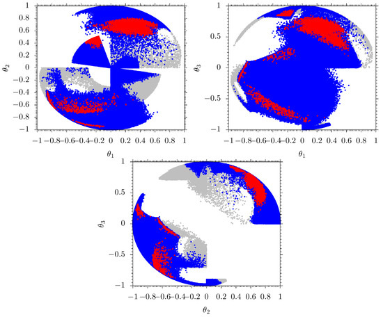
Figure 1.
Grey points satisfy the REWSB and yield LSP neutralinos. The blue points are the subset of gray points that satisfy the LEP bound, Higgs mass bound, B-physics, and LHC sparticle mass bounds. Red points are a subset of blue points that satisfy 5 Planck relic density bounds.
In our scanning, we see in the - plane, the range of the red points for is , but most of the points are concentrated from to , while for it is . Also, for most of the points are concentrated from to and to . For and , we have red point solutions almost everywhere in the entire range except for the where the solutions are in the to range. On the other hand, blue points are more or less everywhere in the plot. In - plane, the concentration of red points favors the positive range as in the case of - plane. We also see a small concentration of red points in the negative range for the small negative value of and for the large negative value of . Blue points are almost everywhere in the plot in contrast to the - plane, as we have the density of points around the center of the plot. In the - plane, here again, we see the concentration of red points favors the positive range for and . But we also see a small concentration of red points in the negative range smaller than that of the positive range for a small negative value of and a large negative value of . For all points, we see a polarization-like pattern compared to other planes and having no points in the center of the plot.
We calculate the (SSB) parameters given in Equation (2). We present the results in Figure 2 and Figure 3, color coding is the same as that of Figure 1. We present the – plane in the top left panel. Red points are in the range from [−5, 6] TeV for , but the large density favors the positive range from [4, 6] TeV. The density of red points smaller than that of the positive range was also concentrated for the negative values [−5, −2] TeV for . For the blue points, we have solutions almost everywhere for from [−5, 6] TeV except around 1 TeV. We also see the concentration of red points at [1, 3] TeV in the positive range and [−3.5, −1] TeV in the negative range for . For the blue points, we have solutions almost everywhere from [−5, 4.5] TeV for . In short, we see a polarisation kind of pattern for red and blue points having no points in the center. We present the – plane in the top right panel. We see almost a similar pattern to that of the – plane but a slight difference can be observed in that the red points are concentrated at [2, 3] TeV and [−3.5, −2] TeV for , and at [4, 7] TeV and [−2, −6] TeV for . For blue points, we have solutions for everywhere from [−5, 4.5] TeV, and for , [−6, 7.5] TeV except in the middle. In short, for all the points, we again see a similar pattern as that of the – plane. Finally, we see the – plot in the bottom panel. Similar to the two gaugino plots, here too we see a similar polarization pattern in solutions. The only difference is that since the ranges of and are relatively larger than , the plot in – looks slim.
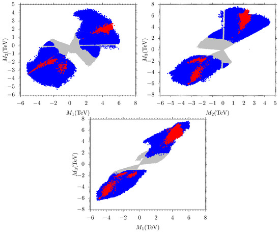
Figure 2.
Plots of results in –, –, and – planes. The color coding and the panel description are the same as in Figure 1.
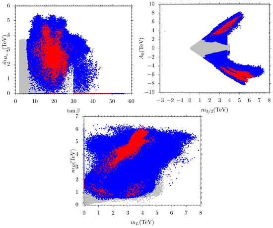
Figure 3.
Plots in –, , and – planes. The color coding and the panel description are the same as in Figure 1.
In Figure 3, we present the –, –, and – planes. Color coding is the same as in Figure 1. In the plane, we see that the red points solution is with TeV but most of the points concentrate in the range to . For blue points, we have a solution for and TeV. In the plane, most of the red points concentrate in the range [2, 7] TeV for and TeV to TeV for . But it can be seen that red solutions favor .
In the – plane we see most of the concentrations of red points at [2, 4.5] TeV for and at [3, 6] TeV for . For the blue points, we have solutions almost everywhere from [0, 7.9] TeV for and from [0.5, 6.5] TeV for .
In Figure 4 we present – and – planes. The panel description and color coding are the same as in Figure 1. As we know LHC is a color particle machine and among the color sparticles, gluinos are the smoking guns for SUSY signals. As we have seen before we have heavy and also relatively heavy left-handed and right-handed scalars, consequentially we have heavy gluinos and stops. For both red and blue points, gluino mass is in the range of 2.2 TeV to 15 TeV, and stop mass is from 0.1 TeV to 11 TeV. It should be noted that at the 100 TeV collider with 30 integrated luminosity, gluino () mass can be probed up to 11 TeV and 17 TeV via heavy flavor decays and via light flavor decays, respectively, and stop () mass up to 11 TeV can be discovered [55,56,57,58]. In the right panel, we display the plot in the – plane. Here we see that both red and blue points are in the range [0.8, 9] TeV. This implies that we have heavier higgsinos.
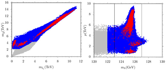
Figure 4.
Plots of results in and planes. The color coding and the panel description are the same as in Figure 1.
We now present results with the LSP neutralino mass and the masses of other particles of our model that are possibly light, i.e., , A, , and masses in Figure 5. The description and color coding are the same as in Figure 1. The solid black lines show the mass degeneracy between the listed particles and for plane, indicates the region. In the top left panel, we present a plot in the plane. We see that there are a couple of red points that have . In this scenario, correct relic density is achieved when a pair of LSP neutralinos annihilates into a CP-odd Higgs. It should be noted that for 1.7 TeV is excluded for 30 [59]. In addition to it at Run 2, Run 3, and HL-LHC the CP-odd Higgs A with 10 can be excluded for masses 1 TeV, 1.1 TeV, and 1.4 TeV, respectively. We hope that future research will be able to investigate such solutions [60,61].
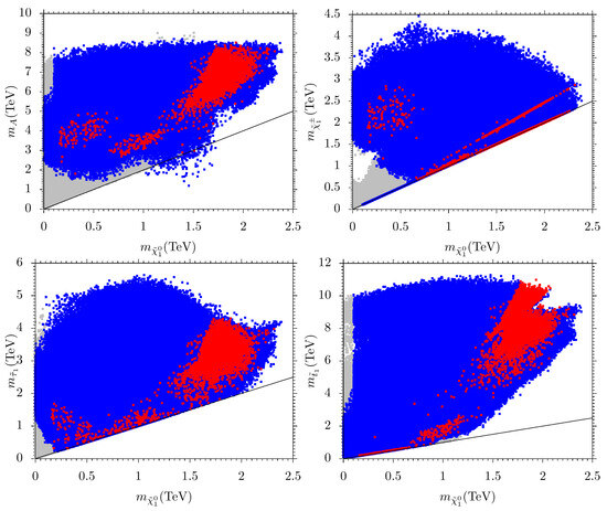
Figure 5.
Plots in –, –, – and – planes. Color coding and panel description are the same as in Figure 1.
In the top right panel, we show a plot in the plane. If we do not care about Planck2018 relic density bounds, we have a neutralino and chargino degenerate masses solution from [0.1, 2.4] TeV but the degenerate masses solution is compatible with Planck2018 bounds from [0.7, 2.3] TeV range. The Ref. [62] has reported the 95% exclusion for sleptons as well as SM-boson-mediated decays of and . It can be seen that the charginos heavier than 300 GeV are safe when they are mass-degenerate with the LSP neutralino. On the other hand in the parameter space where slepton masses are heavier than charginos, these slepton-mediated decays will not take place. Since we also have heavier NLSP chargino solutions, we hope that such solutions will be probed in future LHC searches. In the lower left panel, we present the plot in the plane. Here, we observe that the range of red points where is nearly degenerate with is from [0.3, 1.8] TeV but for the blue points the mass degeneracy ranges are from [0.15, 2.1] TeV. Thus we note that our solutions are consistent with the results reported in [63] with 137 at 13 TeV.
In the lower left panel we present the plot in the plane. Here we have red points along the solid line. Such solutions represent scenarios where NLSP stop is mass-degenerate with the LSP neutralino. In such a case, is the dominant decay channel. From the latest study [64], it is evident that in such a scenario the stop mass around 600 GeV has been excluded [65]. Thus, nearly half of our solutions have already been excluded. We anticipate that future studies will investigate the remaining NLSP stop solution in a small mass gap region.
In Figure 6, we present the plots for spin-independent (left) and spin-dependent (right) neutralino–proton scattering cross-section vs. the neutralino mass. We consider the impact of current and future dark matter (DM) searches on our model. In the left panel, the solid black and yellow lines represent the current LUX [66] and XENON1T [67,68] bounds, respectively, whereas the green and red lines depict the projection of future limits [69] of XENON1T with 2 exposure and XENONnT with 20 exposure, respectively. In the right panel, the solid black line represents the current LUX bound [70], the orange line represents the future Lux–Zeplin (LZ) bound [71] and the blue line represents the IceCube DeepCore [72]. It can be seen that most points are consistent with current LUX and XENON1T bounds. Some points will also be investigated by future Xenon experiments. On the other hand, there are some points that are excluded by the current LUX and Xenon1T experiments. Such points represent the scenario where the chargino is the NLSP and the LSP neutralino is bino-higgsino mixed dark matter. We also want to make a comment here that our NLSP stop solutions are constrained by the collider searches below 600 GeV and the remaining solutions are constrained by the LUX and Xenon experiments. We note that points with NLSP mass around 900 GeV ( which is the heaviest NLSP stop in our model) have just below the current LUX and Xenon1T bounds. Thus future DM searches will definitely investigate such solutions.
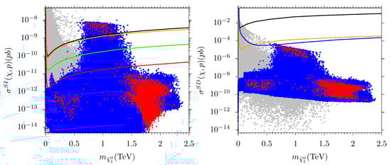
Figure 6.
The spin-independent (left) and spin-dependent (right) neutralino–proton scattering cross-section vs. the neutralino mass. In the left panel, the solid black and orange lines depict the current LUX [66] and XENON1T [67,68] bounds, and the solid green and red lines show the projection of future limits [69] of XENON1T with 2 exposure and XENONnT with 20 exposure, respectively. In the right panel, the black solid line is the current LUX bound [70], the blue solid line represents the IceCube DeepCore [72], and the orange line shows the future LZ bound [71]. The color code in the description is the same as in the Figure 1.
In the right panel, the black solid line represents the current LUX bound [70], the orange line represents the future Lux–Zeplin (LZ) bound [71] and the blue line represents the IceCube DeepCore [72]. Here we see that all solutions are consistent with current and future dark matter searches.
To be specific, we also present a table of benchmark points from our data which explain the various scenarios of our discussion. In Table 1, all points satisfy the constraints described in Section 3, and masses are given in GeV. Point 1 is an example of a chargino–neutralino coannihilation scenario. Here 0.711 TeV and 0.724 TeV. Point 2 shows a stop–neutralino case where 0.876 TeV and 0.911 TeV. Point 3 represents resonance solutions with 2900 GeV (2919 GeV). Finally, point 3 displays a stau–neutralino scenario with 0.807 TeV and 0.821 TeV. We also note that point 2 and point 4 have 1 TeV which means these are relatively less fine-tuned solutions.

Table 1.
All quantities with mass dimension are in the unit of GeV and . All points satisfy the particle mass bounds, B-physics constraints, and Planck bounds described in Section 3. Point 1 represents chargino–neutralino coannihilation while point 2 represents neutralino–stop coannihilations. Point 3 depicts A-resonance; and finally, point 4 displays neutralino–stau coannihilation.
5. Summary and Conclusions
Because there are a few typos in the supersymmetry-breaking sfermion masses and trilinear soft term, we revisit the phenomenological survey of the intersecting D-brane model with modified soft SUSY terms, focused on the LHC and DM constraints, and predict low-energy SUSY particle spectra. The three-family Pati–Salam models have been constructed systematically in Type IIA string theory on the orientifold with intersecting D6-branes [27]. Our phenomenological survey of this three-family Pati–Salam model has been presented in detail in Section 4. In this work, we display the viable parameter space satisfying the collider and DM bounds along with the Higgs mass bounds. We show that in our present scans, we have A/H-resonance solutions, chargino–neutralino coannihilation, stau–neutralino coannihilation, and stop–neutralino coannihilation. In the case of resonance solutions, is about 2 TeV or so. In the case of chargino–neutralino coannihilation, the NLSP chargino mass can be between 0.7 TeV to 2.3 TeV and the NLSP stau is in the mass range of 0.2 TeV to 1.8 TeV. As far as the NLSP stop solutions are concerned we we have solutions from 0.15 TeV to 0.9 TeV. Most of the parameter space related to this scenario has already been probed by the LHC SUSY searches. It should also be noted that the above-mentioned solutions, except for some of the chargino–neutralino solutions, are consistent with the ongoing and future astrophysical dark matter experiments.
Author Contributions
Investigation, I.K.; Writing—review & editing, W.A. and S.R.; Supervision, T.L. All authors have read and agreed to the published version of the manuscript.
Funding
T.L. is supported in part by the National Key Research and Development Program of China Grant No. 2020YFC2201504, by the Projects No. 11875062, No. 11947302, No. 12047503, and No. 12275333 supported by the National Natural Science Foundation of China, by the Key Research Program of the Chinese Academy of Sciences, Grant NO. XDPB15, by the Scientific Instrument Developing Project of the Chinese Academy of Sciences, Grant No. YJKYYQ20190049, and by the International Partnership Program of Chinese Academy of Sciences for Grand Challenges, Grant No. 112311KYSB20210012. I.K. would like to acknowledge the CAS-TWAS president’s fellowship program.
Data Availability Statement
Data are contained within the article.
Conflicts of Interest
The authors declare no conflicts of interest.
Note
| 1 | The gaugino masses are almost squeezed up to 50% from the previous study, which provided an important contribution in evaluating the sparticle masses from the GUT to electroweak scale in SUSY GUTs. Similarly, the spectrum for , , , and in the negative range are also squeezed up to 50% in our new study. In short, the overall mass spectrum is squeezed from 20% to 50%. Furthermore, we are unable to have the gluino coannihilation channel in our new results, and previously we were expecting to have some points that are important regarding LHC SUSY searches. We have no stop coannihilation in the previous study and in the new study there is stop coannihilation up to 1 TeV for the Planck2018 relic density (within 5) satisfied points. Similarly, we have no stau coannihilation points below 1 TeV consistent with the Planck20018 relic density bounds within 5 and in the new study, there is stau coannihilation below 1 TeV. |
References
- Aad, G.; Abajyan, T.; Abbott, B.; Abdallah, J.; Khalek, S.A.; Abdelalim, A.A.; Aben, R.; Abi, B.; Abolins, M.; AbouZeid, O.S.; et al. Observation of a new particle in the search for the Standard Model Higgs boson with the ATLAS detector at the LHC. Phys. Lett. B 2012, 716, 1–29. [Google Scholar]
- Chatrchyan, S.; Khachatryan, V.; Sirunyan, A.M.; Tumasyan, A.; Adam, W.; Aguilo, E.; Bergauer, T.; Dragicevic, M.; Erö, J.; Fabjan, C.; et al. Observation of a new boson at a mass of 125 GeV with the CMS experiment at the LHC. Phys. Lett. B 2012, 716, 30–61. [Google Scholar]
- Dimopoulos, S.; Raby, S.; Wilczek, F. Supersymmetry and the Scale of Unification. Phys. Rev. D 1981, 24, 1681. [Google Scholar] [CrossRef]
- Marciano, W.J.; Senjanovic, G. Predictions of Supersymmetric Grand Unified Theories. Phys. Rev. D 1982, 25, 3092. [Google Scholar] [CrossRef]
- Amaldi, U.; de Boer, W.; Furstenau, H. Comparison of grand unified theories with electroweak and strong coupling constants measured at LEP. Phys. Lett. B 1991, 260, 447. [Google Scholar] [CrossRef]
- Ellis, J.R.; Kelley, S.; Nanopoulos, D.V. Probing the desert using gauge coupling unification. Phys. Lett. B 1991, 260, 131. [Google Scholar] [CrossRef]
- Langacker, P.; Luo, M.X. Implications of precision electroweak experiments for Mt, ρ0, sin2θW and grand unification. Phys. Rev. D 1991, 44, 817. [Google Scholar] [CrossRef]
- Jungman, G.; Kamionkowski, M.; Griest, K. Supersymmetric Dark Matter. Phys. Rept. 1996, 267, 195. [Google Scholar] [CrossRef]
- Aaboud, M.; Aad, G.; Abbott, B.; Abeloos, B.; Abidi, S.H.; AbouZeid, O.S.; Abraham, N.L.; Abramowicz, H.; Abreu, H.; Abreu, R.; et al. Search for squarks and gluinos in final states with jets and missing transverse momentum using 36 fb−1 of = 13 TeV pp collision data with the ATLAS detector. Phys. Rev. D 2018, 97, 112001. [Google Scholar] [CrossRef]
- Vami, T.A.; ATLAS; CMS. Searches for gluinos and squarks. In Proceedings of the 7th Large Hadron Collider Physics Conference (LHCP 2019), Puebla, Mexico, 20–25 May 2019; Volume 168. [Google Scholar] [CrossRef]
- Sirunyan, A.M.; Tumasyan, A.; Adam, W.; Ambrogi, F.; Asilar, E.; Bergauer, T.; Brandstetter, J.; Brondolin, E.; Dragicevic, M.; Erö, J.; et al. Search for new phenomena with the MT2 variable in the all-hadronic final state produced in proton–proton collisions at = 13 TeV. Eur. Phys. J. C 2017, 77, 710. [Google Scholar] [CrossRef]
- Leggett, T.; Li, T.; Maxin, J.A.; Nanopoulos, D.V.; Walker, J.W. No Naturalness or Fine-tuning Problems from No-Scale Supergravity. arXiv 2014, arXiv:1403.3099. [Google Scholar]
- Leggett, T.; Li, T.; Maxin, J.A.; Nanopoulos, D.V.; Walker, J.W. Confronting Electroweak Fine-tuning with No-Scale Supergravity. Phys. Lett. B 2015, 740, 66. [Google Scholar] [CrossRef]
- Du, G.; Li, T.; Nanopoulos, D.V.; Raza, S. Super-Natural MSSM. Phys. Rev. D 2015, 92, 025038. [Google Scholar]
- Cremmer, E.; Ferrara, S.; Kounnas, C.; Nanopoulos, D.V. Naturally Vanishing Cosmological Constant In N = 1 Supergravity. Phys. Lett. B 1983, 133, 61. [Google Scholar] [CrossRef]
- Ellis, J.R.; Lahanas, A.B.; Nanopoulos, D.V.; Tamvakis, K. No-Scale Supersymmetric Standard Model. Phys. Lett. B 1984, 134, 429. [Google Scholar]
- Ellis, J.R.; Kounnas, C.; Nanopoulos, D.V. Phenomenological SU(1,1) Supergravity. Nucl. Phys. B 1984, 241, 406. [Google Scholar] [CrossRef]
- Ellis, J.R.; Kounnas, C.; Nanopoulos, D.V. No Scale Supersymmetric Guts. Nucl. Phys. B 1984, 247, 373. [Google Scholar] [CrossRef]
- Lahanas, A.B.; Nanopoulos, D.V. The Road to No Scale Supergravity. Phys. Rept. 1987, 145, 1–139. [Google Scholar] [CrossRef]
- Giudice, G.F.; Masiero, A. A Natural Solution to the mu Problem in Supergravity Theories. Phys. Lett. B 1988, 206, 480. [Google Scholar] [CrossRef]
- Berkooz, M.; Douglas, M.R.; Leigh, R.G. Branes intersecting at angles. Nucl. Phys. B 1996, 480, 265. [Google Scholar] [CrossRef]
- Ibanez, L.E.; Marchesano, F.; Rabadan, R. Getting just the standard model at intersecting branes. J. High Energy Phys. 2001, 0111, 2. [Google Scholar]
- Blumenhagen, R.; Kors, B.; Lust, D.; Ott, T. The standard model from stable intersecting brane world orbifolds. Nucl. Phys. B 2001, 616, 3–33. [Google Scholar]
- Cvetič, M.; Shiu, G.; Uranga, A.M. Three-family supersymmetric standardlike models from intersecting brane worlds. Phys. Rev. Lett. 2001, 87, 201801. [Google Scholar] [CrossRef] [PubMed]
- Cvetič, M.; Shiu, G.; Uranga, A.M. Chiral four-dimensional N = 1 supersymmetric type IIA orientifolds from intersecting D6-branes. Nucl. Phys. B 2001, 615, 3. [Google Scholar] [CrossRef]
- Cvetič, M.; Papadimitriou, I.; Shiu, G. Supersymmetric three family SU(5) grand unified models from type IIA orientifolds with intersecting D6-branes. Nucl. Phys. B 2003, 659, 193, Erratum in Nucl. Phys. B 2004, 696, 298. [Google Scholar] [CrossRef][Green Version]
- Cvetic, M.; Li, T.; Liu, T. Supersymmetric patiSalam models from intersecting D6-branes: A Road to the standard model. Nucl. Phys. B 2004, 698, 163. [Google Scholar] [CrossRef]
- Cvetic, M.; Langacker, P.; Li, T.; Liu, T. D6-brane splitting on type IIA orientifolds. Nucl. Phys. B 2005, 709, 241. [Google Scholar] [CrossRef][Green Version]
- Cvetic, M.; Li, T.; Liu, T. Standard-like models as type IIB flux vacua. Phys. Rev. D 2005, 71, 106008. [Google Scholar] [CrossRef]
- Chen, C.-M.; Kraniotis, G.V.; Mayes, V.E.; Nanopoulos, D.V.; Walker, J.W. A supersymmetric flipped SU(5) intersecting brane world. Phys. Lett. B 2005, 611, 156. [Google Scholar] [CrossRef][Green Version]
- Chen, C.-M.; Kraniotis, G.V.; Mayes, V.E.; Nanopoulos, D.V.; Walker, J.W. A K-theory anomaly free supersymmetric flipped SU(5) model from intersecting branes. Phys. Lett. B 2005, 625, 96. [Google Scholar] [CrossRef][Green Version]
- Chen, C.M.; Li, T.; Nanopoulos, D.V. Standard-like model building on type II orientifolds. Nucl. Phys. B 2006, 732, 224. [Google Scholar] [CrossRef]
- Blumenhagen, R.; Cvetic, M.; Langacker, P.; Shiu, G. Toward realistic intersecting D-brane models. Ann. Rev. Nucl. Part. Sci. 2005, 55, 71. [Google Scholar] [CrossRef]
- Pati, J.C.; Salam, A. Lepton Number as the Fourth Color. Phys. Rev. D 1974, 10, 275, Erratum in Phys. Rev. D 1975, 11, 703. [Google Scholar] [CrossRef]
- Chen, C.M.; Li, T.; Mayes, V.E.; Nanopoulos, D.V. A Realistic world from intersecting D6-branes. Phys. Lett. B 2008, 665, 267. [Google Scholar] [CrossRef]
- Chen, C.M.; Li, T.; Mayes, V.E.; Nanopoulos, D.V. Towards realistic supersymmetric spectra and Yukawa textures from intersecting branes. Phys. Rev. D 2008, 77, 125023. [Google Scholar] [CrossRef]
- Li, T.; Nanopoulos, D.V.; Raza, S.; Wang, X.C. A Realistic Intersecting D6-Brane Model after the First LHC Run. J. High Energy Phys. 2014, 1408, 128. [Google Scholar] [CrossRef]
- Sabir, M.; Li, T.; Mansha, A.; Wang, X.C. The supersymmetry breaking soft terms, and fermion masses and mixings in the supersymmetric Pati-Salam model from intersecting D6-branes. J. High Energy Phys. 2022, 4, 89. [Google Scholar] [CrossRef]
- Baer, H.; Paige, F.E.; Protopopescu, S.D.; Tata, X. ISAJET 7.48: A Monte Carlo event generator for p p, anti-p p, and e+ e-reactions. arXiv 2003, arXiv:hep-ph/0001086. [Google Scholar]
- Tevatron Electroweak Working Group; CDF Collaboration; D0 Collab. Combination of CDF and D0 Results on the Mass of the Top Quark. arXiv 2009, arXiv:0903.2503. [Google Scholar]
- Belanger, G.; Boudjema, F.; Pukhov, A.; Singh, R.K. Constraining the MSSM with universal gaugino masses and implication for searches at the LHC. J. High Energy Phys. 2009, 911, 26. [Google Scholar] [CrossRef]
- Baer, H.; Kraml, S.; Sekmen, S.; Summy, H. Dark matter allowed scenarios for Yukawa-unified SO(10) SUSY GUTs. J. High Energy Phys. 2008, 803, 56. [Google Scholar] [CrossRef]
- Patrignani, C.; Agashe, K.; Aielli, G.; Amsler, C.; Antonelli, M.; Asner, D.M.; Baer, H.; Banerjee, S.; Barnett, R.M.; Basaglia, T.; et al. Review of Particle Physics. Chin. Phys. C 2016, 40, 100001. [Google Scholar]
- Aad, G.; Abbott, B.; Abbott, D.C.; Abud, A.A.; Abeling, K.; Abhayasinghe, D.K.; Abidi, S.H.; AbouZeid, O.S.; Abraham, N.L.; Abramowicz, H.; et al. Measurements of the Higgs boson production and decay rates and constraints on its couplings from a combined ATLAS and CMS analysis of the LHC pp collision data at = 7 and 8 TeV. J. High Energy Phys. 2016, 1608, 45. [Google Scholar]
- Slavich, P.; Heinemeyer, S.; Bagnaschi, E.; Bahl, H.; Goodsell, M.; Haber, H.E.; Hahn, T.; Harlander, R.; Hollik, W.; Lee, G.; et al. Higgs-mass predictions in the MSSM and beyond. Eur. Phys. J. C 2021, 81, 450. [Google Scholar] [CrossRef]
- Allanach, B.C.; Djouadi, A.; Kneur, J.L.; Porod, W.; Slavich, P. Precise determination of the neutral Higgs boson masses in the MSSM. J. High Energy Phys. 2004, 9, 44. [Google Scholar] [CrossRef]
- Baer, H.; Brhlik, M. Signals for the minimal gauge-mediated supersymmetry-breaking model at the Fermilab Tevatron collider. Phys. Rev. D 1997, 55, 4463. [Google Scholar] [CrossRef]
- Baer, H.; Brhlik, M.; Castano, D.; Tata, X. b→ s γconstraints on the minimal supergravity model with large tan β. Phys. Rev. D 1998, 58, 015007. [Google Scholar] [CrossRef]
- Babu, K.; Kolda, C. Higgs-mediated B0→μ+μ− in minimal supersymmetry. Phys. Rev. Lett. 2000, 84, 228. [Google Scholar] [CrossRef] [PubMed]
- Dedes, A.; Dreiner, H.; Nierste, U. Correlation of Bs→μ+μ− and (g − 2) μ in minimal supergravity. Phys. Rev. Lett. 2001, 87, 251804. [Google Scholar] [CrossRef] [PubMed]
- Mizukoshi, J.K.; Tata, X.; Wang, Y. Higgs-mediated leptonic decays of Bs and Bd mesons as probes of supersymmetry. Phys. Rev. D 2002, 66, 115003. [Google Scholar] [CrossRef]
- Khachatryan, V.; Sirunyan, A.M.; Tumasyan, A.; Adam, W.; Bergauer, T.; Filipovic, N.; Bencze, G.; Hajdu, C.; Hidas, P.; Horváth, D.; et al. Observation of the rare →μ+μ− decay from the combined analysis of CMS and LHCb data. Nature 2015, 522, 68. [Google Scholar]
- Amhis, Y.; Banerjee, S.; Ben-Haim, E.; Blyth, S.; Bozek, A.; Bozzi, C.; Carbone, A.; Chistov, R.; Chrząszcz, M.; Cibinetto, G.; et al. Averages of b-hadron, c-hadron, and τ-lepton properties as of summer 2014. arXiv 2014, arXiv:1412.7515. [Google Scholar]
- Aghanim, N.; Akrami, Y.; Arroja, F.; Ashdown, M.; Aumont, J.; Baccigalupi, C.; Ballardini, M.; Banday, A.J.; Barreiro, R.B.; Bartolo, N.; et al. Planck 2018 results. I. Overview and the cosmological legacy of Planck. Astron. Astrophys. 2020, 641, A1. [Google Scholar] [CrossRef]
- Cohen, T.; Golling, T.; Hance, M.; Henrichs, A.; Howe, K.; Loyal, J.; Padhi, S.; Wacker, J.G. SUSY Simplified Models at 14, 33, and 100 TeV Proton Colliders. J. High Energy Phys. 2014, 4, 117. [Google Scholar] [CrossRef]
- Arkani-Hamed, N.; Han, T.; Mangano, M.; Wang, L.T. Physics opportunities of a 100 TeV proton–proton collider. Phys. Rept. 2016, 652, 1–49. [Google Scholar] [CrossRef]
- Fan, J.; Jaiswal, P.; Leung, S.C. Jet Observables and Stops at 100 TeV Collider. Phys. Rev. D 2017, 96, 036017. [Google Scholar] [CrossRef]
- Golling, T.; Hance, M.; Harris, P.; Mangano, M.L.; McCullough, M.; Moortgat, F.; Schwaller, P.; Torre, R.; Agrawal, P.; Alves, D.S.M.; et al. Physics at a 100 TeV pp collider: Beyond the Standard Model phenomena. arXiv 2016, arXiv:1606.00947. [Google Scholar] [CrossRef]
- Tumasyan, A.; Adam, W.; Andrejkovic, J.W.; Bergauer, T.; Chatterjee, S.; Damanakis, K.; Dragicevic, M.; Del Valle, A.E.; Fruehwirth, R.; Jeitler, M.; et al. Searches for additional Higgs bosons and for vector leptoquarks in ττ final states in proton-proton collisions at = 13 TeV. arXiv 2022, arXiv:2208.02717. [Google Scholar]
- Baer, H.; Barger, V.; Tata, X.; Zhang, K. Prospects for Heavy Neutral SUSY HIGGS Scalars in the hMSSM and Natural SUSY at LHC Upgrades. Symmetry 2022, 14, 2061. [Google Scholar] [CrossRef]
- Baer, H.; Barger, V.; Tata, X.; Zhang, K. Detecting heavy neutral SUSY Higgs bosons decaying to sparticles at the high-luminosity LHC. arXiv 2022, arXiv:2212.09198. [Google Scholar]
- [ATLAS]. SUSY Summary Plots June 2021. ATL-PHYS-PUB-2021-019. Available online: https://cds.cern.ch/record/2771785/files/ATL-PHYS-PUB-2021-019.pdf (accessed on 25 February 2024).
- Tumasyan, A.; Adam, W.; Andrejkovic, J.W.; Bergauer, T.; Chatterjee, S.; Damanakis, K.; Dragicevic, M.; Escalante Del Valle, A.; Fruehwirth, R.; Jeitler, M.; et al. Search for direct pair production of supersymmetric partners of τ leptons in the final state with two hadronically decaying τ leptons and missing transverse momentum in proton-proton collisions at = 13 TeV. arXiv 2022, arXiv:2207.02254. [Google Scholar]
- Aad, G.; Abbott, B.; Abbott, D.C.; Abud, A.A.; Abeling, K.; Abhayasinghe, D.K.; Abidi, S.H.; AbouZeid, O.S.; Abraham, N.L.; Abramowicz, H.; et al. Search for new phenomena in events with an energetic jet and missing transverse momentum in pp collisions at = 13 TeV with the ATLAS detector. Phys. Rev. D 2021, 103, 112006. [Google Scholar]
- [ATLAS]. SUSY March 2023 Summary Plot Update. ATL-PHYS-PUB-2023-005. Available online: https://atlas.web.cern.ch/Atlas/GROUPS/PHYSICS/PUBNOTES/ATL-PHYS-PUB-2023-005/ (accessed on 25 February 2024).
- Akerib, D.S.; Alsum, S.; Araújo, H.M.; Bai, X.; Bailey, A.J.; Balajthy, J.; Beltrame, P.; Bernard, E.P.; Bernstein, A.; Biesiadzinski, T.P.; et al. Results from a search for dark matter in the complete LUX exposure. Phys. Rev. Lett. 2017, 118, 021303. [Google Scholar] [CrossRef] [PubMed]
- Aprile, E.; Aalbers, J.; Agostini, F.; Alfonsi, M.; Amaro, F.D.; Anthony, M.; Arneodo, F.; Barrow, P.; Baudis, L.; Bauermeister, B.; et al. First Dark Matter Search Results from the XENON1T Experiment. Phys. Rev. Lett. 2017, 119, 181301. [Google Scholar] [CrossRef] [PubMed]
- Collaboration, X.E.N.O.N.; Aprile, E.; Aalbers, J.; Agostini, F.; Alfonsi, M.; Althueser, L.; Amaro, F.D.; Anthony, M.; Arneodo, F.; Baudis, L.; et al. Dark Matter Search Results from a One Ton-Year Exposure of XENON1T. Phys. Rev. Lett. 2018, 121, 111302. [Google Scholar]
- Aprile, E.; Aalbers, J.; Agostini, F.; Alfonsi, M.; Amaro, F.D.; Anthony, M.; Arazi, L.; Arneodo, F.; Balan, C.; Barrow, P.; et al. Physics reach of the XENON1T dark matter experiment. J. Cosmol. Astropart. Phys. 2016, 1604, 27. [Google Scholar] [CrossRef]
- Akerib, D.S.; Alsum, S.; Araújo, H.M.; Bai, X.; Bailey, A.J.; Balajthy, J.; Beltrame, P.; Bernard, E.P.; Bernstein, A.; Biesiadzinski, T.P.; et al. Limits on spin-dependent WIMP-nucleon cross section obtained from the complete LUX exposure. Phys. Rev. Lett. 2017, 118, 251302. [Google Scholar] [CrossRef] [PubMed]
- Akerib, D.S.; Araújo, H.M.; Bai, X.; Bailey, A.J.; Balajthy, J.; Beltrame, P.; Bernard, E.P.; Bernstein, A.; Biesiadzinski, T.P.; Boulton, E.M.; et al. Results on the Spin-Dependent Scattering of Weakly Interacting Massive Particles on Nucleons from the Run 3 Data of the LUX Experiment. Phys. Rev. Lett. 2016, 116, 161302. [Google Scholar] [CrossRef]
- Abbasi, R.; Abdou, Y.; Ackermann, M.; Adams, J.; Ahlers, M.; Andeen, K.; Auffenberg, J.; Bai, X.; Baker, M.; Barwick, S.W.; et al. Limits on a muon flux from neutralino annihilations in the Sun with the IceCube 22-string detector. Phys. Rev. Lett. 2009, 102, 201302. [Google Scholar] [CrossRef]


Disclaimer/Publisher’s Note: The statements, opinions and data contained in all publications are solely those of the individual author(s) and contributor(s) and not of MDPI and/or the editor(s). MDPI and/or the editor(s) disclaim responsibility for any injury to people or property resulting from any ideas, methods, instructions or products referred to in the content. |
© 2024 by the authors. Licensee MDPI, Basel, Switzerland. This article is an open access article distributed under the terms and conditions of the Creative Commons Attribution (CC BY) license (https://creativecommons.org/licenses/by/4.0/).