Abstract
A Friedmann–Lemaitre–Robertson–Walker space–time model with all curvatures is explored in gravity, where R is the Ricci scalar, and T is the trace of the energy–momentum tensor. The solutions are obtained via the parametrization of the scale factor that leads to a model transiting from a decelerated universe to an accelerating one. The physical features of the model are discussed and analyzed in detail. The study shows that gravity can be a good alternative to the hypothetical candidates of dark energy to describe the present accelerating expansion of the universe.
1. Introduction
Observational data such as Planck [1], baryon acoustic oscillations (BAO) [2], the Wilkinson microwave anisotropy probe (WMAP) [3], large-scale structures (LSS) [4], cosmic microwave background radiation (CMBR) [5], and Type-Ia supernova (SNe-Ia) [6,7,8], have become a vital pillar in comprehending modern cosmology. These observations suggest that the universe has undergone a pillar of accelerated expansion twice, viz., early inflation [9,10,11] and late-time acceleration. The inflationary phase has resolved the flatness and horizon problems [9] as well as the entropy problem partially. Acceleration at late-times is supposed to be caused by an unknown component known as dark energy (DE) that occupies approximately two-thirds of the total energy budget of the universe [12,13]. The most widely acknowledged CDM (cold dark matter) model based on Einstein’s theory of general relativity (GR) explains the late-time acceleration phenomenon via a cosmological constant (CC), [14,15], which is characterized by an equation of state (EoS) parameter .
Though the standard model explains various physical phenomena, such as the formation and evolution of the large-scale structure in the early universe and the abundance of matter and energy [16,17], etc., it experiences setbacks such as coincidence and fine-tuning problems [18,19]. Due to these setbacks, researchers have proposed some dynamic candidates for DE. These include quintessence [20], phantom energy [21,22], tachyons [23], Chaplygin gas [24], and k-essence [25]. However, due to the lack of evidence of the existence of any of these forms of DE, a class of researchers are not in favor of accommodating these hypothetical candidates of DE. Instead of such a theoretical form of energy, they prefer to seek some other alternatives to explain acceleration at late times. One way is to modify the action of GR. The modified theories naturally unify early-time inflation and late-time acceleration [26,27]. The most popular modified theories include theories [28,29], scalar Gauss–Bonnet gravity [30], generalized Gauss–Bonnet [31], theory [32], theory [33], and gravity [34].
Among modified gravity theories, initially, the focus was put only on altering the geometrical part of the EH action. Later, explicit coupling of an arbitrary function of the Ricci scalar R and the matter lagrangian was introduced, and a maximal extension of the EH action was proposed [35]. These theories came to be known as the gravity theories [36]. In 2011, Harko et al. [37], through non-minimal general coupling between geometry and matter, introduced gravity, where T is the trace of the stress–energy tensor. Exotic imperfect fluids or quantum effects provide the rationale for selecting T as a Lagrangian argument. The authors argued that the variation of the stress–energy tensor with respect to the metric is represented by a source term. Consequently, the matter content, as well as the geometrical part, contribute to cosmic acceleration. Furthermore, neither ghosts nor Laplacian instabilities exist in this theory [38]. Additionally, the theory has passed observational tests on intra- and extra-galactic scales. This extraordinary behavior and observational validity set this theory apart from other theories of gravity by producing notable signatures and effects. Therefore, gravity has gained a lot of interest and rose to the top of the list of potential solutions in many contexts on galactic and intra-galactic scales.
Jamil et al. [39] reconstructed some gravity models and showed that the dust fluid reproduces CDM, phantom-non-phantom era and phantom cosmology. Azizi [40] studied wormhole solutions in the framework of gravity. Alvarenga et al. [41] studied the evolution of scalar cosmological perturbations in the metric formalism. Sharif et al. [42] studied the energy conditions for the FLRW universe with perfect fluid. Pasqua et al. [43] reconstructed modified holographic Ricci dark energy. Alves et al. [44] explored gravitational waves in this theory. Momeni et al. [45] presented a study of the generalized second law of thermodynamics in the scope of gravity. Das et al. [46] generated a set of solutions describing the interior of a compact star which admits conformal motion. Using a perfect fluid as the only matter content, Shabani and Ziaie [47] studied classical bouncing solutions in a flat FLRW background. Deb et al. [48] explored the physical features of anisotropic strange stars beyond the standard maximum mass limit in gravity. Elizalde and Khurshudyan [49] discussed the formation of specific static wormhole models. Ordines and Carlson [50] investigated changes in the earth’s atmospheric models coming from the modified theory of gravity (for more details, see [51,52] and the references therein).
On the other hand, it is also well known that prior to the current accelerating expansion, the universe had undergone a decelerated phase in the past. However, constructing viable scaling models that allow the universe to transition from a decelerating to an accelerating phase is still a challenging task. An alternative is to seek the solutions of the field equations under an assumption which would be consistent with the observed kinematics of the universe. This phenomenon has piqued the interest of many researchers. Some theorists working in this area have attempted to study it by constructing cosmological models using geometrical parameters, such as the parametrization of the deceleration parameter, Hubble parameter, or scale factor, which can provide the transition from past deceleration to present acceleration [53,54,55,56]. Most of these models have been studied in homogeneous and isotropic backgrounds [57,58,59,60,61,62,63,64,65], but some studies have also been considered in homogeneous but anisotropic backgrounds [66,67,68,69,70,71,72].
Knowing the EoS of DE is one of the biggest challenges in theoretical physics [73,74,75,76,77] as well as in observational cosmology today [78,79]. The observations seem to favor an evolving EoS for DE [80,81]. Considering all curvatures , the present study deals with a transit FLRW model in gravity. We consider a scale factor as proposed in Ref. [82]. We investigate the nature of matter and its sources, which exhibit cosmological evolution as suggested by the theoretical background and supported by the various observations. In particular, we seek to answer whether gravity could be a possible alternative to various hypothetical forms of DE.
The work is organized as follows. The model and field equations followed by their solutions are presented in Section 2. The geometrical behavior of the deceleration parameter is also presented in the same section, and the constraints for a physically realistic scenario are obtained therein. Thereafter, the nature of matter is examined. As compared to GR, in the theory of gravity, due to coupling, some additional terms arise in the energy–momentum tensor. These extra terms may be considered as coupled matter or energy, which may behave as either perfect fluid or DE. The nature of this coupled matter is examined in Section 3. The behaviour of effective matter is studied in Section 4. The results are summarized in Section 5.
2. The Model in Gravity
The spatially homogeneous and isotropic FLRW space–time metric is given as follows:
where , , a is the scale factor, and k represents the geometrical curvature of the universe, i.e., implies a flat universe, is a closed universe, and is an open universe. We consider the energy–momentum tensor of the matter as follows:
where is the energy density and is the thermodynamic pressure of the matter. In comoving coordinates, , where is the four-velocity of the fluid that satisfies the condition .
Harko et al. [37] considered some functional forms of gravity models. The authors mentioned that in the theory of gravity, the field equations are governed by the choice of the source of matter. Therefore, by choosing suitable matter fields, a different cosmological model is obtained by choosing a different functional form for f. In their paper, those authors took the simplest case, i.e., , showing the equivalence with a cosmological model with an effective cosmological constant, which varies with Hubble parameter, i.e., . It was also shown that gravitational coupling is no longer constant, but is now a function of time, viz., , where a prime represents a derivative with respect to the argument. Thus, the term in the gravitational action modifies the gravitational interaction between matter and curvature. Although there is not any fundamental basis for considering a liner combination of R and T, the authors showed that the choice of for the dust matter leads to the power-law expansion of the universe, , where depends on the coupling parameter .
The choice also corresponds to GR with an additional matter content on the right side of the field equations. This allows for a wider variety of behaviour, which reduces to GR when . The right side of the field equations are similar (but not the same) to general relativity, containing a fluid with viscosity or heat conduction. Hence, the entropy problem could be solved using the theory. Several problems, such as the fine-tuning problem, coincidence problem, and cosmological constant problem can be solved by the dynamic in theory, and it can still satisfy observations [83]. The variable parameter occurring in the theory may be written as a function of T where T is the trace of , and is sometimes called “ gravity”. Hence, this means that a variable can be derived naturally from gravity via a Lagrangian formulation. However, the choice has not always been met with a positive reception by the scientific community in a few papers [84,85]. Such criticism has been addressed in Ref. [86] recently. Very recently, Jaekel et al. [87], on some observational grounds, proposed that and models should be ruled out. However, their analysis is biased. Staying on the conservative side, those authors considered the age of the universe as more than 14.16 Gyrs. Also, there are some other constraints that were followed in their study. These models are, at the very least, still viable at lower redshift limits, as shown in Ref. [88]. We shall return further to the comments in Ref. Jaekel et al. [87] later in the conclusion.
Moreover, it was shown earlier [89] that when reconstructing , an exponential solution implies that . A similar result is true for power-law solutions, but in this case, , where is a constant. It is well known that the conservation equation does not necessarily hold in gravity—see Appendix A. Moreover, a scalar field with flat potential was studied earlier in the theory of gravity [90], looking for conditions for energy conservation. Surprisingly, it was found that the expression had the same form as before, viz., . Hence, this linear form of has a significant physical and mathematical basis. Whilst being simple, this form allows one to investigate salient points of this theory. Hence, this simple form is popular with most researchers in the field. In the present study, we also consider this form.
The field equations in gravity with the system of units , are obtained as follows:
where a prime represents the derivative with respect to T. The above equation for , i.e., , where , simplifies as follows:
For the (1) metric and the energy–momentum tensor (2), the above equation yields the following:
It is vital to note that in the theory of gravity, both and do not reflect the effective pressure and energy density as in GR. Indeed, the coupling between matter and gravity adds some additional terms visible on the RHS of the field equations. Additional contributions can be collected in terms of geometrical effective pressure and energy density. This can be associated with the dark sector. If the modified gravity sector is responsible for the late time accelerated phase, then the additional terms can be interpreted as DE. This is the convention that we adopt in this work. We term the additional terms with as “coupled matter” or “coupled energy”. Therefore, to distinguish the “main” matter from the “coupled” matter or energy, we write and , which represents the coupled matter or energy.
Now, Einstein’s equations with the cosmological constant on the right-hand side of the field equations are as follows:
Comparing this with (4), we notice that a variable in gravity may be defined as follows:
Hence, we see that variable arises naturally in gravity. Thus, additional matter–geometry coupling terms work as a variable cosmological parameter. This can assist in solving the fine-tuning problem, coincidence problem, and cosmological constant problem. In addition, observations can also be satisfied [83].
Ideally, the solutions of (5) and (6) are supposed to be obtained by solving the conservation equation. However, as far as gravity, as mentioned earlier, is concerned, the usual conservation equation in GR is not satisfied [37]. However, only in a few cases does the chosen function lead to a conservation equation holding true. In Ref. [90], two of the present authors studied such a case. For a complete discussion on this, we would like to refer to a recent study [91]. Secondly, if one tries to compute the analogue of the conservation equation in gravity, this leads to very complicated expressions, and even more so if one inserts this into the Friedmann Equation (5). This is extremely difficult to solve; hence, most researchers resort to assuming some form of scale factor, Hubble parameter, deceleration parameter, equation of state parameter, etc.
The transition from a decelerated phase to an accelerated phase must be present in any realistic model. However, due to our lack of knowledge of dark energy, constructing viable scaling models that allow the universe to transition from a decelerating phase to an accelerating phase is still a challenging task. An alternative is to seek solutions of field equations under an assumption which would be consistent with the observed kinematics of the universe. This phenomenon has piqued the interest of many researchers. Some theorists working in this area have attempted to study it by constructing cosmological models using geometrical parameters, such as the parametrization of the deceleration parameter, Hubble parameter, or scale factor, which can provide the transition from past deceleration to present acceleration, and be consistent with observations. Many researchers have considered similar geometrical evolutions (for an extensive list, see Refs. given in [92]). Some authors [68,93,94,95] have studied another form of the hybrid scale factor, which also describes the transition from the decelerated to accelerated expansion of the universe. Apart from these works, there are a plethora of similar works.
We see that Equations (5) and (6) consist of three unknowns, i.e., , and H. Hence, to determine a solution, one extra assumption is required. We have considered the simple parametrization of the scale factor as recently studied by Mishra and Dua [82]:
where , , and are arbitrary constants.
Now, let us discuss the scale factor considered here further. The approach to seek solutions of the field equations under an assumption which would be consistent with the observed kinematics of the universe is known as cosmography, which has been extensively studied in the literature. In Ref. [90], two of the present authors cited many such works conducted earlier. While following this reverse approach, the authors obtained similar scale factors.
As far as the parameters are concerned in solution (7), we have tried to consider the most general form. Later, while investigating, we realized that some of the parameters are just scaling and shifting parameters. Therefore, we dropped them out. If we would have analyzed without those parameters, it would be a very specific study, and one could argue why such a particular study must be considered. In any case, there are many papers in the literature where such parameters are included.
The Hubble parameter, yields the following:
Using , where is the present value of a, and z is the redshift, one obtains the relationship [82]:
where , is the present time. Using the above relationship, the Hubble parameter is obtained in terms of redshift z as follows:
Similarly, the deceleration parameter, , in terms of the redshift, is as follows:
where , and is the present value of the deceleration parameter.
Recently, using the 51 points data set [96] and the 1048 points Pantheon SNe-Ia data set [97] with = 67.77 km [98], Mishra and Dua [82] obtained observational constraints on and p, and reported the best-fitted values and with the data set and and with the Pantheon data set.
Figure 1 plots the deceleration parameter q versus redshift z for the best-fitted values mentioned above. We observe that the universe transits from deceleration () to acceleration () at a redshift od for the data and for the Pantheon data.
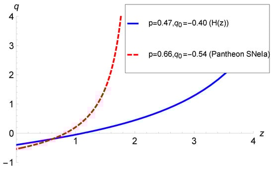
Figure 1.
Deceleration parameter q in terms of redshift z with the best-fitted values of p and .
We note the following. Firstly, the deceleration parameter for the adopted form of the scale factor describes a transition from a deceleration in the past to acceleration in the future. Secondly, the values of p and the current deceleration parameter occur in our equation for the deceleration parameter . To plot our deceleration parameter, as in Figure 1, we use the values of and p obtained from observations, as mentioned above. The calculated values of the transition redshift work out to be 0.8 and 1.2. Whilst this is somewhat higher than the value for the CDM model, it is within the error bounds [99]. Thirdly, the usually quoted values of are based on the CDM model, and values for alternative theories or models could be somewhat different whilst the model has the required salient features.
The main objectives of our study are as follows:
- Investigating the nature of matter in the presence of which the model can yield the desired evolution of the universe.
- Examining the role of gravity.
- Comparing and distinguishing outcomes from those of Einstein’s gravity.
Using (7) and (8) in (5) and (6), we obtain the energy density and pressure of matter as follows:
The vital requirement is now to corroborate that the assumption we chose to find a solution results in a realistic cosmological model, e.g., . We note that requires in all the three models .
Let us examine the behavior of actual matter. The EoS parameter of actual matter provides the following:
Since is a scaling parameter and is just a shifting parameter, the only crucial parameter in this study is p. Therefore, we set and to study the behavior of the EoS parameter for the best-fitted values ( data) and (Pantheon data). Figure 2 and Figure 3 depict the behavior of matter with the and Pantheon data, respectively.
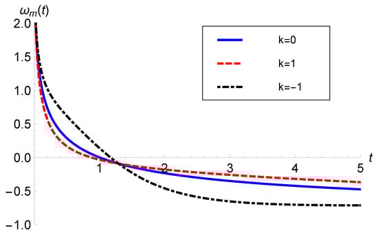
Figure 2.
versus t with ( data) and .
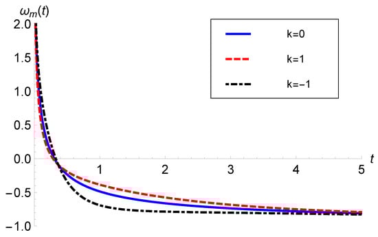
Figure 3.
versus t with (Pantheon data) and .
Analytically, we find that for all three spatial curvature models, at , and as . Therefore, starts with a finite value with the evolution and approaches the cosmological constant at late times. Hence, the matter exhibits a unified description of all kinds of matter, including stiff matter (), radiation (), dust (), quintessence (), and a cosmological constant (), in the same order as is required for unified cosmological evolution.
3. The Behavior of Coupled Matter
The energy density and pressure of coupled matter are obtained as follows:
In all three spatial curvature models, we note that the energy density of coupled matter is negative at very early stages of evolution, and turns out to be positive after a particular length of time. Since becomes zero at the transition time, it is noteworthy to use the EoS parameter to study the behavior of coupled matter as would diverge at that instant of time. Alternatively, we study the implications of the energy conditions, which are stated as follows:
- Null energy conditions (NEC): ;
- Weak energy conditions (WEC): , ;
- Strong energy conditions (SEC): ;
- Dominant energy conditions (DEC): .
Figure 4 shows the behavior of energy density for a flat model, which shows that the WEC is violated at very early times. We observe the same behavior in closed and open models. Although the energy density of a field in classical physics is strictly positive, the energy density in quantum field theory can be negative due to quantum coherence effects [100]. The Casimir effect [101,102] and squeezed states of light [103] are two familiar examples which have been studied experimentally. As a result, all the known pointwise energy conditions in GR, such as the WEC and NEC, are allowed to be violated. Even for a scalar field in flat Minkowski spacetime, it can be proven that the existence of quantum states with negative energy density is inevitable [100]. The violation of the WEC of coupled matter can be advocated by any of such mechanisms.
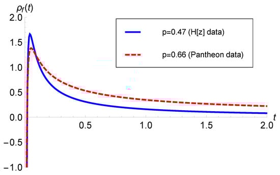
Figure 4.
versus t for flat model with ( data), (Pantheon data) and .
The expression for is obtained as follows:
Since and , the above expression implies for flat and closed models. For , Figure 5 plots , implying the NEC also holds good for the open model.
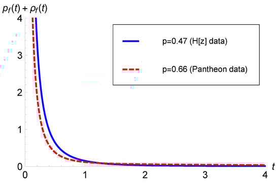
Figure 5.
versus t for with .
Further, following is the expression of ,
Figure 6 and Figure 7 plot with and Pantheon data, respectively. Due to the domination of the term at very early times, starts from a negative value, later it becomes positive, and, after attaining a maximum value, it starts decreasing and finally approaches zero at late times. Hence, the DEC is satisfied, except during the very early stages of evolution. This shows that coupled matter behaves as a phantom type of DE during the very early stage of evolution. Mechanically, phantom matter can originate from scalar fields with a global minimum in their effective potential [104], from higher-order curvature terms in higher-order theories of gravity [105,106,107,108,109], from bulk viscous stress due to particle production [110], in Brans–Dicke and non-minimally coupled scalar field theories [111], in strange effective quantum field theory [112,113], and by some other means (for details, see [114]). Most of these disparate prescriptions require the weakly coupled scalar field to be displaced from its equilibrium state. However, in the present study, we do not need any such hypothetical form of DE; rather, it is the natural outcome of matter–geometry coupling of gravity.
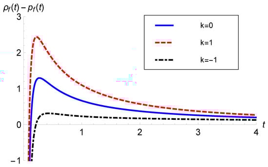
Figure 6.
versus t with ( data), and .
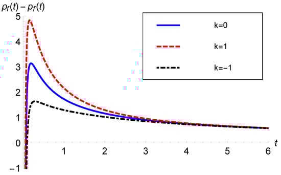
Figure 7.
versus t with (Pantheon data) and .
Lastly, we have the follows:
Figure 8 and Figure 9 depict the behavior of with data and Pantheon data, respectively. In both models, becomes negative at late times. Hence, the SEC was violated during late-time evolution in all three models. This shows that coupled matter contributes as a quintessence type of DE and accelerates the expansion of the universe at late times. Again, it is interesting to note that no physical quintessence kind of matter is required to drive the late-time acceleration. Rather, the matter–geometry coupling of gravity plays the role of DE in this model.
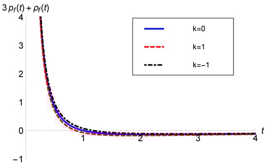
Figure 8.
versus t with ( data) and .
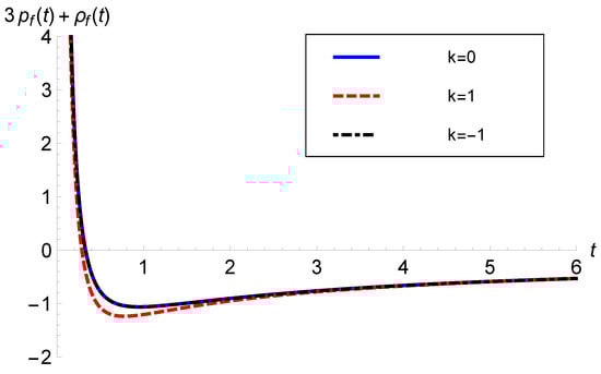
Figure 9.
versus t with (Pantheon data) and .
Thus, we observed that the main matter behaves as a phantom kind of DE, whereas the coupled matter acts as a quintessence kind of DE. However, since the model’s evolution in this study is controlled by effective matter, this makes it more crucial for the study of the behavior of effective matter together with individual matter sources.
4. The Behavior of Effective Matter
The energy density and pressure of effective matter can be obtained from and , which also can be read from Equations (11) and (12) with . Similarly, the EoS of effective matter can be read from Equation (13) with , which implies that effective matter behaves similarly to GR. We note that effective matter obeys the WEC for all three curvature models. The behavior of effective matter with and Pantheon data is illustrated in Figure 10 and Figure 11, respectively.
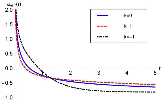
Figure 10.
versus t with ( data).
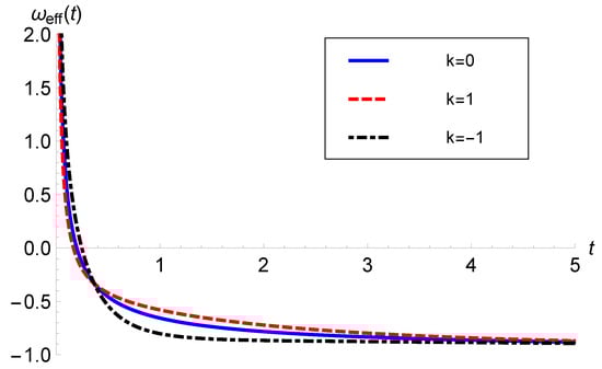
Figure 11.
versus t with (Pantheon data).
The behavior of effective matter follows the same pattern as the matter discussed in Section 2. This can be observed by comparing Figure 2 and Figure 3 with Figure 10 and Figure 11. Therefore, the interpretation made for actual matter applies to the effective one, too. We note that the overall behavior of the effective matter follows the behavioral characteristics of the scalar field. Kinetic energy dominates the scalar potential early on in the evolution of the model. Thus, the scalar field behaves similarly to stiff matter. During inflation, this leads to extremely fast expansion driven by negative pressure. Just as a cosmological constant exerts stress at late times, the scalar field does as well as the potential term dominates the kinetic term during this era. It is important to note that the energy density is different to that during inflation. However, the effective matter in this study does not accommodate early inflation, but it effectively comprises the behavior of the hybrid scale factor considered in this study to transition from a decelerated era to the present accelerating era.
5. Conclusions
In this paper, we studied an FLRW space–time model filled with a perfect fluid in the framework of gravity, where for all spatially curved models. In order to find solutions, we chose parametrization of the scale factor, , where and , which yields a deceleration parameter consistent with early deceleration to a late-time acceleration phase for the parameters that best fit the data, viz. data) and (Pantheon data) [82]. The transition takes place at a redshift of for the data and for the Pantheon data.
Figure 2 and Figure 3 depict the behavior of matter for the and Pantheon data, respectively. The kinematical dynamics of the model are independent of the theory and were studied earlier by Mishra and Dua [82] in the Brans–Dicke theory. To eschew repetition, the kinematical study is not presented in this paper. We found that a physically realistic cosmological model is possible only for . We investigated the role of gravity.
As compared to GR, in gravity, due to coupling, if we look at the field equations on the right-hand side, there are extra terms. These extra terms may be termed coupled matter, which may behave either as perfect fluid or DE. First and foremost, we ascertain that all three spatial curvature models () demand a positive coupling constant () to have a physically realistic scenario, i.e., to obey the WEC. Further, we identified the nature of the main matter and coupled matter to exhibit the transition from early deceleration to late time accelerated expansion. The main attributes of the models are the individual behaviors of primary matter and coupled matter, which are summarized below:
- The primary matter exhibits the characteristics of all kinds of matter, viz., stiff matter (), radiation (), dust (), quintessence (), and a cosmological constant (), in the same order as is required to depict the cosmic history, including the transition from a decelerating to an accelerating universe.
- The coupled matter satisfies the NEC throughout the evolution of the universe. However, it violates the WEC and the NEC during very early stages of evolution. It also violates the SEC at late times, which shows that the coupled matter contributes to quintessence DE.
Since effective matter governs how the universe evolves, in this investigation, it was crucial to study the behavior of effective matter separately from individual matter sources. Effective matter follows an evolving EoS, as shown in Figure 10 and Figure 11. Effective matter exhibits a dual nature, i.e., a perfect fluid at early times and exotic matter at late times, which is consistent with observations. If geometric parameters govern the kinematic behavior in the theory of gravity, then the way of behaving of the effective matter is not altered. Hence, as compared to GR, effective matter behaves similarly. It is also noteworthy to caption that all three spatial curvature models (flat, closed, and open) are indistinguishable as far as either the individual matter contents or effective matter are concerned.
It is noteworthy to mention here that Malik et al. [115] considered a more general form of the scale factor to study the bouncing cosmological scenario. The crucial element in facilitating a successful bounce is the violation of the NEC around the bouncing point, which the authors found in their study. However, our model does not violate the NEC at any stage of evolution. Moreover, the hybrid scale factor explored in the present study is completely different from that considered by Malik et al. and does not encounter a bounce at any stage. One can easily verify that the scale factor studied here is not a particular case of the one considered in [115]. However, there might be a possibility that the present model is one cycle of a bounce.
Further, we comment on Ref. [87]. Their conclusion is that gravity is not able to provide a full cosmological scenario and should be ruled out as a modified gravity alternative to the DE phenomena. This is strongly based on the assumption that the universe is old enough to accommodate the existence of galactic globular clusters with ages of at least Gyrs. This can be seen in their statement, “stay on the conservative side, let us consider that the universe should be older than 14.16 Gyrs”. In addition, the authors, in Equation (24), mentioned the age of the universe as . However, they considered only the positive error (upper bound) in their work.
In justification of the above comment, we would like to acknowledge another study [88], where the authors challenged some of the available models by arguing that, although the low evolution of models can be reasonably supported by the available data, there is considerable discrepancy in high () dynamics in comparison with standard CDM cosmology. Thus, the proposal of ruling out in Ref. [87] may be valid for the higher redshift zone. The gravity model studied here is still viable for lower redshift, i.e., for late times.
We mentioned earlier that if one tries to substitute the analogue of the conservation equation into the Friedmann Equation (5), solving the resulting equation is difficult. However, in Ref. [87], the authors conducted a broad study of models with , where n is a constant. Their conclusion of Section III was that “ cosmologies have a viable parameter space to describe the late-time cosmological observables”. Our model has in their notation, so it also falls into the category of having “a viable parameter space to describe the late-time cosmological observables”. Secondly, those authors discussed the effects of radiation. This approach is highly problematic for at least two reasons: (1) theory is not valid for pure radiation with , and (2) as the authors themselves acknowledge, radiation plays a negligible role in the late universe. However, the authors still wrote evolution equations, including terms with , but without making any comments on how they computed the derivatives of f for . Even if they initially considered a model, after substituting in the field equations, an incorrect (from the point of view of the theory) model was obtained. Since the theory is not valid for , any pathological behavior shown for this case is not relevant for the understanding of the theory. Therefore, their study confirms through cosmological observations the validity of the correctly formulated and applied theory [116].
As a final remark, the model explains late-time acceleration without including any form of hypothetical exotic matter, indicating that gravity can be a good alternative to DE. In the absence of any fundamental physical phenomenon, the matter–geometry coupling terms simply can be interpreted as a variable cosmological parameter, which not only explains the current accelerating expansion but can also resolve problems such as the fine-tuning problem and the coincidence problem, whilst being consistent with cosmological observations [83].
Author Contributions
Conceptualization, S.J., V.S. and A.B.; methodology, V.S., S.J. and A.B.; software, V.S. and S.J.; validation, V.S. and A.B.; formal analysis, V.S.; data curation, V.S.; writing—original draft preparation, S.J.; writing—review and editing, V.S. and A.B.; visualization, V.S. and S.J.; supervision, V.S. and A.B.; project administration, A.B.; funding acquisition, S.J. and A.B. All authors have read and agreed to the published version of the manuscript.
Funding
This work was based on the research supported in part by the National Research Foundation of South Africa (Grant Numbers: 118511).
Data Availability Statement
The original contributions presented in the study are included in the article, further inquiries can be directed to the corresponding author.
Acknowledgments
The authors are grateful to the reviewers for their critical comments, which led to the improvement of the manuscript. A.B. acknowledges private correspondence with Tiberio Harko regarding some aspects of gravity.
Conflicts of Interest
The authors declare no conflicts of interest. The funders had no role in the design of the study; in the collection, analyses, or interpretation of data; in the writing of the manuscript; or in the decision to publish the results.
Appendix A
In this appendix, we confirm that our model is non-conservative. Setting , in Equation (10) of Ref. [117], the covariant derivative of the field equations in gravity lead to the following:
where we considered .
For , the above equation reduces to the following:
Since , p, and H are known in our model, one may verify that the above equation is violated for our study, which supports the fact that the conservation equation does not hold in gravity, in general.
References
- Aghanim, N.; Akrami, Y.; Ashdown, M.; Aumont, J.; Baccigalupi, C.; Ballardini, M.; Banday, A.J.; Barreiro, R.B.; Bartolo, N.; Basak, S.; et al. Planck 2018 results. VI. Cosmological parameters. Astron. Astrophys. 2018, 641, A6. [Google Scholar]
- Anderson, L.; Aubourg, E.; Bailey, S.; Beutler, F.; Bhardwaj, V.; Blanton, M.; Bolton, A.S.; Brinkmann, J.; Brownstein, J.R.; Burden, A.; et al. The clustering of galaxies in the SDSS-III Baryon Oscillation Spectroscopic Survey: Baryon Acoustic Oscillations in the data release 9 spectroscopic galaxy sample. Mon. Not. Roy. Astron. Soc. 2013, 427, 3435. [Google Scholar] [CrossRef]
- Bennett, C.L.; Larson, D.; Weiland, J.L.; Jarosik, N.; Hinshaw, G.; Odegard, N.; Smith, K.M.; Hill, R.S.; Gold, B.; Halpern, M.; et al. Nine-Year Wilkinson Microwave Anisotropy Probe (WMAP) Observations: Final maps and results (WMAP Collaboration). Astrophys. J. Suppl. 2013, 208, 20. [Google Scholar] [CrossRef]
- Spergel, D.N.; Verde, L.; Peiris, H.V.; Komatsu, E.; Nolta, M.R.; Bennett, C.L.; Halpern, M.; Hinshaw, G.; Jarosik, N.; Kogut, A.; et al. First year Wilkinson Microwave Anisotropy Probe (WMAP) observations: Determination of cosmological parameters. Astrophys. J. Suppl. 2003, 148, 175–194. [Google Scholar] [CrossRef]
- Netterfield, C.B.; Ade, P.A.; Bock, J.J.; Bond, J.R.; Borrill, J.; Boscaleri, A.; Coble, K.; Contaldi, C.R.; Crill, B.P.; de Bernardis, P.; et al. A measurement by BOOMERANG of multiple peaks in the angular power spectrum of the cosmic microwave background. Astrophys. J. 2002, 571, 604. [Google Scholar] [CrossRef]
- Riess, A.G.; Filippenko, A.V.; Challis, P.; Clocchiatti, A.; Diercks, A.; Garnavich, P.M.; Gilliland, R.L.; Hogan, C.J.; Jha, S.; Kirshner, R.P.; et al. Observational evidence from supernovae for an accelerating universe and a cosmological constant. Astrophy. J. 1998, 116, 1009. [Google Scholar] [CrossRef]
- Perlmutter, S.; Aldering, G.; Goldhaber, G.; Knop, R.A.; Nugent, P.; Castro, P.G.; Deustua, S.; Fabbro, S.; Goobar, A.; Groom, D.E.; et al. Measurements of Ω and Λ from 42 high-redshift supernovae. Astrophy. J. 1999, 517, 565. [Google Scholar] [CrossRef]
- Schmidt, B.P.; Suntzeff, N.B.; Phillips, M.M.; Schommer, R.A.; Clocchiatti, A.; Kirshner, R.P.; Garnavich, P.; Challis, P.; Leibundgut, B.R.U.N.O.; Spyromilio, J.; et al. The high-z supernova search: Measuring cosmic deceleration and global curvature of the universe using type Ia supernovae. Astrophy. J. 1998, 507, 46. [Google Scholar] [CrossRef]
- Guth, A.H. Inflationary universe: A possible solution to the horizon and flatness problems. Phys. Rev. 1981, 23, 347. [Google Scholar] [CrossRef]
- Albrecht, A.; Steinhardt, P.J. Cosmology for grand unified theories with radiatively induced symmetry breaking. Phys. Rev. Lett. 1982, 48, 1220–1223. [Google Scholar] [CrossRef]
- Linde, A. A new inflationary universe scenario: A possible solution of the horizon, flatness, homogeneity, isotropy and primordial monopole problems. Phys. Lett. B 1982, 108, 389–393. [Google Scholar] [CrossRef]
- Frieman, J.A.; Turner, M.S.; Huterer, D. Dark Energy and the accelerating universe. Ann. Rev. Astron. Astrophys. 2008, 46, 385. [Google Scholar] [CrossRef]
- Copeland, E.J.; Sami, M.; Tsujikawa, S. Dynamics of dark energy. Int. J. Mod. Phys. D 2006, 15, 1753–1936. [Google Scholar] [CrossRef]
- Komatsu, E.; Dunkley, J.; Nolta, M.R.; Bennett, C.L.; Gold, B.; Hinshaw, G.; Jarosik, N.; Larson, D.; Limon, M.; Page, L.E.A.; et al. Five-year Wilkinson microwave anisotropy probe (WMAP) observations: Cosmological interpretation. Astrophys. J. Suppl. 2009, 180, 330–376. [Google Scholar] [CrossRef]
- Sahni, V.; Starobinsky, A.A. The case for a positive cosmological Lambda-term. Int. J. Mod. Phys. D 2000, 9, 373–444. [Google Scholar] [CrossRef]
- Popolo, A.D. Non-baryonic dark matter in cosmology. AIP Conf. Proc. 2013, 1548, 2–63. [Google Scholar]
- Popolo, A.D.; Delliou, M.L.; Lee, X. Correlations in the matter distribution in CLASH galaxy clusters. Phys. Dark Universe 2019, 26, 100342. [Google Scholar] [CrossRef]
- Weinberg, S. The cosmological constant problem. Rev. Mod. Phys. 1989, 61, 1. [Google Scholar] [CrossRef]
- Astashenok, A.V.; Popolo, A.D. Cosmological measure with volume averaging and the vacuum energy problem. Class. Quantum Grav. 2012, 29, 085014. [Google Scholar] [CrossRef]
- Martin, J. Quintessence: A mini-review. Mod. Phys. Lett. A 2008, 23, 1252–1265. [Google Scholar] [CrossRef]
- Caldwell, R.R.; Kamionkowski, M.; Weinberg, N.N. Phantom energy: Dark energy with ω < −1 causes a cosmic doomsday. Phys. Rev. Lett. 2003, 91, 071301. [Google Scholar] [PubMed]
- Tonry, J.L.; Schmidt, B.P.; Barris, B.; Candia, P.; Challis, P.; Clocchiatti, A.; Coil, A.L.; Filippenko, A.V.; Garnavich, P.; Hogan, C.; et al. Cosmological results from high-z supernovae. Astrophys. J. 2003, 594, 1. [Google Scholar] [CrossRef]
- Padmanabhan, T.; Choudhury, T.R. Can the clustered dark matter and the smooth dark energy arise from the same scalar field? Phys. Rev. D 2002, 66, 081301. [Google Scholar] [CrossRef]
- Bento, M.C.; Bertolami, O.; Sen, A.A. Generalized Chaplygin gas, accelerated expansion, and dark-energy-matter unification. Phys. Rev. D 2002, 66, 043507. [Google Scholar] [CrossRef]
- Takeshi, C.; Okabe, T.; Yamaguchi, M. Kinetically driven quintessence. Phys. Rev. D 2000, 62, 023511. [Google Scholar]
- Nojiri, S.I.; Odintsov, S.D. Unifying inflation with ΛCDM epoch in modified f (R) gravity consistent with Solar System tests. Phys. Lett. B 2007, 657, 238–245. [Google Scholar] [CrossRef]
- Nojiri, S.I.; Odintsov, S.D. Unified cosmic history in modified gravity: From f (R) theory to Lorentz non-invariant models. Phys. Rep. 2011, 505, 59–144. [Google Scholar] [CrossRef]
- Sotiriou, T.P.; Faraoni, V. f (R) theories of gravity. Rev. Mod. Phys. 2010, 82, 451. [Google Scholar] [CrossRef]
- Felice, A.D.; Tsujikawa, S. f (R) theories. Living Rev. Relativ. 2010, 13, 3. [Google Scholar] [CrossRef]
- Nojiri, S.I.; Odintsov, S.D. Modified Gauss–Bonnet theory as gravitational alternative for dark energy. Phys. Lett. B 2005, 631, 1–6. [Google Scholar] [CrossRef]
- Cognola, G.; Elizalde, E.; Nojiri, S.I.; Odintsov, S.D.; Zerbini, S. String-inspired Gauss-Bonnet gravity reconstructed from the universe expansion history and yielding the transition from matter dominance to dark energy. Phys. Rev. D 2007, 75, 086002. [Google Scholar] [CrossRef]
- Mandal, S.; Sahoo, P.K. A complete cosmological scenario in teleparallel gravity. Eur. Phys. J. Plus 2020, 135, 706. [Google Scholar] [CrossRef]
- Järv, L.; Rünkla, M.; Saal, M.; Vilson, O. Nonmetricity formulation of general relativity and its scalar-tensor extension. Phys. Rev. D 2018, 97, 124025. [Google Scholar] [CrossRef]
- Xu, Y.; Harko, T.; Shahidi, S.; Liang, S.D. Weyl type f (Q, T) gravity, and its cosmological implications. Eur. Phys. J. C 2020, 80, 449. [Google Scholar] [CrossRef]
- Bertolami, O.; Lobo, F.S.N.; Paramos, J. Nonminimal coupling of perfect fluids to curvature. Phys. Rev. D 2008, 78, 064036. [Google Scholar] [CrossRef]
- Harko, T.; Lobo, F.S.N. f (R, Lm) gravity. Eur. Phys. J. C 2010, 70, 373–379. [Google Scholar] [CrossRef]
- Harko, T.; Lobo, F.S.; Nojiri, S.I.; Odintsov, S.D. f (R, T) gravity. Phy. Rev. D 2011, 84, 024020. [Google Scholar] [CrossRef]
- Tretyakov, P.V. Cosmology in modified f (R, T)-gravity. Eur. Phys. J. C 2018, 78, 896. [Google Scholar] [CrossRef]
- Jamil, M.; Momeni, D.; Raza, M.; Myrzakulov, R. Reconstruction of some cosmological models in f (R, T) cosmology. Eur. Phys. J. C 2012, 72, 1999. [Google Scholar] [CrossRef]
- Azizi, T. Wormhole geometries in f (R, T) Gravity. Int. J. Theor. Phys. 2013, 52, 3486. [Google Scholar] [CrossRef]
- Alvarenga, F.G.; de la Cruz-Dombriz, A.; Houndjo, M.J.S.; Rodrigues, M.E.; Sáez-Gómez, D. Dynamics of scalar perturbations in f (R, T) gravity. Phys. Rev. D 2013, 87, 103526. [Google Scholar] [CrossRef]
- Sharif, M.; Rani, S.; Myrzakulov, R. Analysis of F (R, T) gravity models through energy conditions. Eur. Phys. J. Plus 2013, 128, 123. [Google Scholar] [CrossRef]
- Pasqua, A.; Chattopadhyay, S.; Khomenkoc, I. A reconstruction of modified holographic Ricci dark energy in f (R, T) gravity. Can. J. Phys. 2013, 91, 632. [Google Scholar] [CrossRef]
- Alves, M.E.S.; Moraes, P.H.R.S.; de Araujo, J.C.N.; Malheiro, M. Gravitational waves in f (R, T) and f (R, Tϕ) theories of gravity. Phys. Rev. D 2016, 94, 024032. [Google Scholar] [CrossRef]
- Momeni, D.; Moraes, P.H.R.S.; Myrzakulov, R. Generalized second law of thermodynamics in f (R, T) theory of gravity. Astrophys. Space Sci. 2016, 361, 228. [Google Scholar] [CrossRef]
- Das, A.; Rahaman, F.; Guha, B.K.; Ray, S. Compact stars in f (R, T) gravity. Eur. Phys. J. C 2016, 76, 654. [Google Scholar] [CrossRef]
- Shabani, H.; Ziaie, A.H. Bouncing cosmological solutions from f (R, T) gravity. Eur. Phys. J. C 2018, 78, 397. [Google Scholar] [CrossRef]
- Deb, D.; Ketov, S.V.; Maurya, S.K.; Khlopov, M.; Moraes, P.H.R.S.; Ray, S. Exploring physical features of anisotropic strange stars beyond standard maximum mass limit in gravity. Mon. Not. Astron. Soc. 2019, 485, 5652. [Google Scholar] [CrossRef]
- Elizalde, E.; Khurshudyan, M. On wormhole formation in f (R, T) gravity: Varying Chaplygin gas and barotropic fluid. Phys. Rev. D 2018, 98, 123525. [Google Scholar] [CrossRef]
- Ordines, T.M.; Carlson, E.D. Limits on f (R, T) gravity from Earth’s atmosphere. Phys. Rev. D 2019, 99, 104052. [Google Scholar] [CrossRef]
- Singh, V.; Beesham, A. Plane symmetric model in f (R, T) gravity. Eur. Phys. J. Plus 2020, 135, 319. [Google Scholar] [CrossRef]
- Singh, V.; Beesham, A. LRS Bianchi I model with constant expansion rate in f (R, T). Astrophys. Space Sci. 2020, 13, 125. [Google Scholar] [CrossRef]
- Banerjee, N.; Das, S. Acceleration of the universe with a simple trigonometric potential. Gen. Relativ. Gravit. 2005, 37, 1695–1703. [Google Scholar] [CrossRef]
- Akarsu, A.; Dereli, T. Cosmological models with linearly varying deceleration parameter. Int. J. Theor. Phys. 2012, 51, 612–621. [Google Scholar] [CrossRef]
- Mishra, B.; Tripathy, S.K.; Tarai, S. Cosmological models with a hybrid scale factor in an extended gravity theory. Mod. Phys. Lett. A 2018, 33, 1850052. [Google Scholar] [CrossRef]
- Pradhan, A.; Goswami, G.; Beesham, A. The reconstruction of constant jerk parameter with f (R, T) gravity. J. High Energy Astrophys. 2023, 38, 12–21. [Google Scholar] [CrossRef]
- Chawla, C.; Mishra, R.K.; Pradhan, A. String cosmological models from early deceleration to current acceleration phase with varying G and Λ. Eur. Phys. J. Plus 2012, 127, 137. [Google Scholar] [CrossRef]
- Mishra, R.K.; Chand, A. Cosmological models in alternative theory of gravity with bilinear deceleration parameter. Astrophys. Space Sci. 2016, 361, 259. [Google Scholar] [CrossRef]
- Mishra, R.K.; Dua, H.; Chand, A. Bianchi-III cosmological model with BVDP in modified f (R, T) theory. Astrophys. Space Sci. 2018, 363, 112. [Google Scholar] [CrossRef]
- Mishra, R.K.; Dua, H. Phase transition of cosmological model with statistical techniques. Astrophys. Space Sci. 2020, 365, 131. [Google Scholar] [CrossRef]
- Tiwari, R.K.; Sofuoglu, D. Quadratically varying deceleration parameter in f (R, T) gravity. Int. J. Geom. Methods Mod. Phys. 2020, 17, 2030003. [Google Scholar] [CrossRef]
- Katore, S.D.; Gore, S.V. ΛCDM cosmological models with quintessence in f (R) theory of gravitation. J. Astrophys. Astron. 2020, 41, 12. [Google Scholar] [CrossRef]
- Ahmed, N.; Fekry, M.; Shaker, A.A. Transition from decelerating to accelerating universe with quadratic equation of state in f (R, T) gravity. NRIAG J. Astron. Geophys. 2019, 8, 198–203. [Google Scholar] [CrossRef]
- Tiwari, R.K.; Sofuoglu, D.; Beesham, A. FRW universe in f (R, T) gravity. Int. J. Geom. Methods Mod. Phys. 2021, 18, 2150104. [Google Scholar] [CrossRef]
- Pradhan, A.; Garg, P.; Dixit, A. FRW cosmological models with cosmological constant in f (R, T) theory of gravity. Can. J. Phys. 2021, 999, 741–753. [Google Scholar] [CrossRef]
- Pradhan, A.; Saha, B.; Rikhvitsky, V. Bianchi type-I transit cosmological models with time dependent gravitational and cosmological constants: Reexamined. Indian J. Phys. 2015, 89, 503–513. [Google Scholar] [CrossRef]
- Yadav, A.K. Cosmological constant dominated transit universe from the early deceleration phase to the current acceleration phase in Bianchi-V spacetime. Chin. Phys. Lett. 2012, 29, 079801. [Google Scholar] [CrossRef][Green Version]
- Tripathy, S.K.; Mishra, B.; Khlopov, M.; Ray, S. Cosmological models with a hybrid scale factor. Int. J. Mod. Phys. 2021, 30, 2140005. [Google Scholar] [CrossRef]
- Tarai, S.; Ray, P.P.; Mishra, B.; Tripathy, S.K. Effect of bulk viscosity in cosmic acceleration. Int. J. Geom. Methods Mod. Phys. 2022, 19, 2250060. [Google Scholar] [CrossRef]
- Mishra, B.; Tripathy, S.K.; Tarai, S. Accelerating models with a hybrid scale factor in extended gravity. J. Astrophys. Astron. 2021, 42, 2. [Google Scholar] [CrossRef]
- Tiwari, R.K.; Beesham, A.; Mishra, S.; Dubey, V. Anisotropic Cosmological Model in a Modified Theory of Gravitation. Universe 2021, 7, 226. [Google Scholar] [CrossRef]
- Jokweni, S.; Singh, V.; Beesham, A. LRS Bianchi-I Transit Cosmological Models in f (R, T) Gravity. Phys. Sci. Forum 2023, 7, 34. [Google Scholar] [CrossRef]
- Linder, E.V. Exploring the expansion history of the universe. Phys. Rev. Lett. 2003, 90, 091301. [Google Scholar] [CrossRef]
- Ray, S.; Mukhopadhyay, U.; Duttachowdhury, S.B. Dark energy models with a time-dependent gravitational constant. Int. J. Mod. Phys. D 2007, 16, 1791. [Google Scholar] [CrossRef]
- Mukhopadhyay, U.; Ray, S.; Duttachowdhury, S.B. Λ-CDM universe: A phenomenological approach with many possibilities. Int. J. Mod. Phys. D 2008, 17, 301. [Google Scholar] [CrossRef]
- Linder, E.V. The dynamics of quintessence, the quintessence of dynamics. Gen. Rel. Grav. 2008, 40, 329–356. [Google Scholar] [CrossRef]
- Ray, S.; Rahaman, F.; Mukhopadhyay, U.; Sarkar, R. Variable equation of state for generalized dark energy model. Int. J. Theor. Phys. 2011, 50, 2687–2696. [Google Scholar] [CrossRef]
- Knop, R.A.; Aldering, G.; Amanullah, R.; Astier, P.; Blanc, G.; Burns, M.S.; Conley, A.; Deustua, S.E.; Doi, M.; Ellis, R.S.; et al. New constraints on ΩM, ΩΛ, and Ω from an independent set of 11 high-redshift supernovae observed with the Hubble Space Telescope. Astrophys. J. 2003, 598, 102. [Google Scholar] [CrossRef]
- Tegmark, M.; Blanton, M.R.; Strauss, M.A.; Hoyle, F.; Schlegel, D.; Scoccimarro, R.; Vogeley, M.S.; Weinberg, D.H.; Zehavi, I.; Berlind, A.; et al. The three-dimensional power spectrum of galaxies from the sloan digital sky survey. Astrophys. J. 2004, 606, 702. [Google Scholar] [CrossRef]
- Huterer, D.; Turner, M.S. Probing dark energy: Methods and strategies. Phys. Rev. D 2001, 64, 123527. [Google Scholar] [CrossRef]
- Huterer, D.; Cooray, A. Uncorrelated estimates of dark energy evolution. Phys. Rev. D 2005, 71, 023506. [Google Scholar] [CrossRef]
- Mishra, R.K.; Dua, H. Evolution of FLRW universe in Brans-Dicke gravity theory. Astrophys. Space Sci. 2021, 366, 6. [Google Scholar] [CrossRef]
- Basilakos, S. Solving the main cosmological puzzles with a generalized time varying vacuum energy. Astron. Astrophys. 2009, 508, 575. [Google Scholar] [CrossRef]
- Saha, B. Interacting Scalar and Electromagnetic Fields in f (R, T) Theory of Gravity. Int. J. Theor. Phys. 2015, 54, 3776. [Google Scholar] [CrossRef]
- Fisher, S.B.; Carlson, E.D. Reexamining f (R, T) gravity. Phys. Rev. D 2019, 100, 064059. [Google Scholar] [CrossRef]
- Harko, T.; Moraes, P.H. Comment on Reexamining f (R, T) gravity. Phys. Rev. D 2020, 101, 108501. [Google Scholar] [CrossRef]
- Jaekel, A.P.; da Silva, J.P.; Velten, H. Revisiting f (R, T) cosmologies. Phys. Dark Univ. 2024, 43, 101401. [Google Scholar] [CrossRef]
- Velten, H.; Carames, T.R.P. Cosmological inviability of f (R, T) gravity. Phys. Rev. D 2017, 95, 123536. [Google Scholar] [CrossRef]
- Singh, C.P.; Singh, V. Reconstruction of modified f (R, T) f (R, T) gravity with perfect fluid cosmological models. Gen. Relativ. Grav. 2014, 46, 1696. [Google Scholar] [CrossRef]
- Singh, V.; Beesham, A. The f (R, Tϕ) gravity models with conservation of energy–momentum tensor. Eur. Phys. J. C 2018, 78, 564. [Google Scholar] [CrossRef]
- Bertini, N.R.; Velten, H. Fully conservative f (R, T) gravity and Solar System constraints. Phys. Rev. D 2023, 107, 124005. [Google Scholar] [CrossRef]
- Singh, V.; Beesham, A. A time-varying deceleration parameter for unified description of cosmological evolution. Int. J. Geom. Meth. Mod. Phys. 2018, 15, 1850145. [Google Scholar] [CrossRef]
- Narawade, S.A.; Koussour, M.; Mishra, B. Observational Constraints on Hybrid Scale Factor in f (Q, T) Gravity with Anisotropic Space-Time. Annalen Der Physik 2023, 535, 2300161. [Google Scholar] [CrossRef]
- Singh, S.S.; Anjana Devi, L. Interacting anisotropic dark energy with hybrid expansion in f (R, T) gravity. New Astr. 2022, 90, 101656. [Google Scholar] [CrossRef]
- Aydiner, E. Late time transition of Universe and the hybrid scale factor. Eur. Phys. J. C 2022, 82, 39. [Google Scholar] [CrossRef]
- Magana, J.; Amante, M.H.; Garcia-Aspeitia, M.A.; Motta, V. The Cardassian expansion revisited: Constraints from updated Hubble parameter measurements and type Ia supernova data. Mon. Not. R. Astron. Soc. 2018, 476, 1036–1049. [Google Scholar] [CrossRef]
- Scolnic, D.M.; Jones, D.O.; Rest, A.; Pan, Y.C.; Chornock, R.; Foley, R.J.; Huber, M.E.; Kessler, R.; Narayan, G.; Riess, A.G.; et al. The complete light-curve sample of spectroscopically confirmed SNe Ia from Pan-STARRS1 and cosmological constraints from the combined pantheon sample. Astrophys. J. 2018, 859, 101. [Google Scholar] [CrossRef]
- Macaulay, E.; Nichol, R.C.; Bacon, D.; Brout, D.; Davis, T.M.; Zhang, B.; Bassett, B.A.; Scolnic, D.; A. Möller, A.; D’Andrea, C.B.; et al. First cosmological results using Type Ia supernovae from the Dark Energy Survey: Measurement of the Hubble constant. Mon. Not. R. Astron. Soc. 2019, 486, 2184–2196. [Google Scholar] [CrossRef]
- Kumar, D.; Jain, D.; Mahajan, S.; Mukherjee, A.; Rana, A. Constraints on the transition redshift using Hubble phase space portrait. Int. J. Mod. Phys. D 2023, 32, 2350039. [Google Scholar] [CrossRef]
- Epstein, H.; Glaser, V.; Jaffe, A. Nonpositivity of the energy density in quantized field theories. Nuovo Cimento 1965, 36, 1016. [Google Scholar] [CrossRef]
- Lamoreaux, S.K. Demonstration of the Casimir Force in the 0.6 to 6 μm Range. Phys. Rev. Lett. 1997, 78, 5. [Google Scholar] [CrossRef]
- Mohideen, U.; Roy, A. Precision measurement of the Casimir force from 0.1 to 0.9 μm. Phys. Rev. Lett. 1998, 81, 4549. [Google Scholar] [CrossRef]
- Wu, L.A.; Kimble, H.J.; Hall, J.L.; Wu, H. Generation of squeezed states by parametric down conversion. Phys. Rev. Lett. 1986, 57, 2520. [Google Scholar] [CrossRef] [PubMed]
- Linde, A.D. Phase transitions in gauge theories and cosmology. Rep. Prog. Phys. 1985, 42, 389. [Google Scholar] [CrossRef]
- Barrow, J.D.; Ottewil, A. The stability of general relativistic cosmological theory. J. Phys. A Math. Gen. 1983, 16, 2757. [Google Scholar] [CrossRef]
- Hawking, S.W.; Luttrell, J.C. Higher derivatives in quantum cosmology: (I). The isotropic case. Nucl. Phys. B 1984, 247, 250. [Google Scholar] [CrossRef]
- Whitt, B. Fourth-order gravity as general relativity plus matter. Phys. Lett. B 1984, 145, 176. [Google Scholar] [CrossRef]
- Mijic, M.B.; Morris, M.B.; Suen, W.W. The R2 cosmology: Inflation without a phase transition. Phys. Rev. D 1986, 34, 2934. [Google Scholar] [CrossRef] [PubMed]
- Pollock, M.D. On the initial conditions for super-exponential inflation. Phys. Lett. B 1988, 215, 635. [Google Scholar] [CrossRef]
- Barrow, J.D. String-driven inflationary and deflationary cosmological models. Nucl. Phys. B 1988, 310, 743. [Google Scholar] [CrossRef]
- Torres, D.F. Quintessence, superquintessence, and observable quantities in Brans-Dicke and nonminimally coupled theories. Phys. Rev. D 2002, 66, 043522. [Google Scholar] [CrossRef]
- Nojiri, S.; Odintsov, S.D. Quantum de Sitter cosmology and phantom matter. Phys. Lett. B 2003, 562, 147. [Google Scholar] [CrossRef]
- Nojiri, S.; Odintsov, S.D. Effective equation of state and energy conditions in phantom/tachyon inflationary cosmology perturbed by quantum effects. Phys. Lett. B 2003, 571, 1. [Google Scholar] [CrossRef]
- Piao, Y.S.; Zhang, Y.Z. Phantom inflation and primordial perturbation spectrum. Phys. Rev. D 2004, 70, 063513. [Google Scholar] [CrossRef]
- Malik, A.; Naz, T.; Rauf, A.; Shamir, M.F.; Yousaf, Z. f (R, T) Gravity Bouncing Universe with Cosmological Parameters. Eur. Phys. J. Plus 2024, 139, 276. [Google Scholar] [CrossRef]
- Harko, T.; (Babes-Bolyai University, 1 Kogalniceanu Street, Cluj, Romania). Private communication, 2024.
- Baffou, E.H.; Kpadonou, A.V.; Rodrigues, M.E.; Houndjo, M.J.S.; Tossa, J. Cosmological viable f (R, T) dark energy model: Dynamics and stability. Astrophys. Space Sci. 2015, 356, 173–180. [Google Scholar] [CrossRef]
Disclaimer/Publisher’s Note: The statements, opinions and data contained in all publications are solely those of the individual author(s) and contributor(s) and not of MDPI and/or the editor(s). MDPI and/or the editor(s) disclaim responsibility for any injury to people or property resulting from any ideas, methods, instructions or products referred to in the content. |
© 2024 by the authors. Licensee MDPI, Basel, Switzerland. This article is an open access article distributed under the terms and conditions of the Creative Commons Attribution (CC BY) license (https://creativecommons.org/licenses/by/4.0/).