Combined Studies Approach to Rule Out Cosmological Models Which Are Based on Nonlinear Electrodynamics

Abstract

We apply a combined study in order to investigate the dynamics of cosmological models incorporating nonlinear electrodynamics (NLED). The study is based on the simultaneous investigation of such fundamental aspects as stability and causality, complemented with a dynamical systems investigation of the involved models, as well as Bayesian inference for parameter estimation. We explore two specific NLED models: the power-law and the rational Lagrangian. We present the theoretical framework of NLED coupled with general relativity, followed by an analysis of the stability and causality of the various NLED Lagrangians. We then perform a detailed dynamical analysis to identify the ranges where these models are stable and causal. Our results show that the power-law Lagrangian model transitions through various cosmological phases, evolving from a Maxwell radiation-dominated state to a matter-dominated state. For the rational Lagrangian model, including the Maxwell term, stable and causal behavior is observed within specific parameter ranges, with critical points indicating the evolutionary pathways of the universe. To validate our theoretical findings, we perform Bayesian parameter estimation using a comprehensive set of observational data, including cosmic chronometers, baryon acoustic oscillation (BAO) measurements, and supernovae type Ia (SNeIa). The estimated parameters for both models align with the expected values for the current universe, particularly the matter density ${\Omega }_m$ and the Hubble parameter h. However, the parameters of the models are not tightly constrained within the prior ranges. Our combined studies approach rules out the mentioned models as an appropriate description of the cosmos. Our results highlight the need for further refinement and exploration of NLED-based cosmological models to fully integrate them into the standard cosmological framework.

1. Introduction

The present paradigm of cosmology includes an early period of inflationary expansion [1], a stage of decelerated matter dominance [2], and accelerated expansion at late times [3,4]. These distinct phases are well supported by observational evidence and are essential components of the standard cosmological model [5]. These dynamics can be achieved by introducing various material contents into Einstein’s theory of general relativity [6,7] or by appropriately modifying the theory itself [8].

Nonlinear electrodynamics (NLED) has been a subject of interest since the early 20th century, primarily due to its potential to address issues not explained by classical Maxwellian electrodynamics. One of the first significant models was introduced by Born and Infeld in 1934; it aimed to eliminate the singularities associated with the self-energy of point charges [9]. NLED theories have since been studied extensively for their ability to describe high-intensity electromagnetic fields and their applications in various areas of physics, including cosmology and astrophysics [10,11,12]. In cosmology, NLED can provide alternative mechanisms for inflation, structure formation, and the late-time accelerated expansion of the universe [13,14]. These models are particularly valuable for their potential to offer insights into the early universe’s dynamics and the nature of dark energy and dark matter.

In the context of cosmological models, NLED has been extensively studied, offering alternative mechanisms for early-universe inflation, structure formation, and late-time accelerated expansion. Various Lagrangians have been proposed to capture the nonlinear effects of electrodynamics in different cosmological scenarios. For instance, the Born–Infeld-type Lagrangian, $L=-{\beta }^2(\sqrt{1+{\displaystyle \frac{F}{2{\beta }^2}}-{\displaystyle \frac{G^2}{16{\beta }^4}}}-1)$, has been analyzed in early-universe models, FRW cosmologies, and Bianchi universes, with a focus on the squared sound speed $c_s^2$ [13,15,16,17,18,19,20,21]. Another model, represented by $L=-{\beta }^2[{(1+{\displaystyle \frac{\beta F}{\sigma }}-{\displaystyle \frac{\beta \gamma G^2}{2\sigma }})}^{\sigma }-1]$, explores nonsingular universes and bouncing scenarios, demonstrating that the NLED behaves as a cosmological constant at early and late times [22]. Additionally, the Lagrangian $L=-{\displaystyle \frac{1}{{\mu }_{o}4}}F+\alpha F^2+\beta G^2$ has been studied extensively in the context of magnetic universes, inflation, and singularity-free scenarios within FRW cosmologies [23,24,25,26,27]. The Lagrangian $L=-{\displaystyle \frac{1}{{\mu }_{o}4}}F+\alpha F^2$ has been analyzed primarily for early-time expansion, inflation, and singularity-free models in FRW cosmologies [19,21,23,24,28,29,30]. Other notable Lagrangians include $L=-{\displaystyle \frac{F}{2\beta F+1}}$, which has been studied in FRW and Bianchi I universes, showing early-time acceleration without singularities [31,32,33,34], and $L=-F{e}^{-\alpha F}$, which addresses inflation, singularity-free scenarios, and the squared sound speed $c_s^2$ [29,35]. These studies highlight the diverse applications and significant potential of NLED in addressing key questions in cosmology, from early-universe dynamics to the late-time accelerated expansion.

The stability and causality analysis of NLED models ensures their physical viability, especially when considering cosmological applications. One of the critical indicators of stability is the behavior of the squared sound speed (SSS), defined as $c_s^2=dp/d\rho$ [36,37]. A stable cosmological model requires a positive SSS ($c_s^2>0$) to prevent the uncontrolled growth of energy density perturbations, which leads to classical instabilities known as gradient instabilities [38]. Additionally, the SSS must not exceed the local speed of light ($c_s^2\le 1$) to avoid superluminal propagation, which would violate causality [39,40,41]. Early works on NLED, such as [25], laid the foundation for these analyses, and subsequent studies, including [21], have provided detailed discussions on the bounds of the SSS and their implications for the stability and causality of NLED models. Ensuring these conditions are met is important for the theoretical consistency and observational compatibility of NLED-based cosmological models. Similarly, the Lagrangian $L=-F{e}^{-\alpha F}$ has been studied for its implications in inflationary scenarios and singularity-free models, with specific focus on ensuring that $c_s^2$ remains within the acceptable range to avoid instabilities [29,35]. Ensuring the stability and causality of NLED models through $c_s^2$ analysis is a theoretical exercise and a necessary step in validating these models against observational data and ensuring their applicability in describing the universe’s evolution.

The present paper explores several cosmological models based on NLED, so the background radiation goes beyond Maxwell’s radiation. Specifically, we investigate NLED models as potential candidates to replicate the observed dynamics of the universe. The novelty of the present investigation is in the combined study we perform through using different complementary tools: (1) the tools of dynamical systems theory, which are useful to expose the asymptotic cosmological dynamics of the models, i.e., to uncover those solutions which are generic and truly relevant; (2) the study of the instabilities which are due to small perturbations of the cosmic background filled with non-Maxwellian radiation, as well as of the tachyonic instabilities which arise due to violation of causality; and (3) a parameter fitting investigation through implementing a Bayesian analysis of the relevant cosmological parameters. The latter study allows us to determine the values of the model parameters that best match the empirical data, providing a robust test of the theoretical models against real-world observations. This procedure enables us to quantify the degree of agreement between the theoretical predictions and the observed data, thus assessing the viability of the models. In addition, by constraining the parameter values, we can reduce the uncertainty in the model predictions, leading to more precise cosmological insights. The dynamical systems tools, in the meantime, allow one to inspect the global (asymptotic) dynamics of the cosmological models in some phase space. The equilibrium asymptotic configurations amount to those generic solutions which are preferred by the system of differential equations on which the cosmological model is based. Attractor solutions represent those cosmological stages which the system naturally evolves to in the asymptotic future. Meanwhile, source critical points represent those asymptotic cosmological stages in the past from where the system evolves into the future. Saddle equilibrium points represent transient stages to which the system is temporarily attracted but from where it is repelled into the future attractor. The importance of the stability study has been already established.

The importance of the present study lies in the power of the combined study we perform here. There are separate parameter fitting studies as well as dynamical systems and stability investigations of several cosmological models which are based on nonlinear electromagnetic fields as the sources of gravitation. According to these studies some models can successfully explain the inflationary stage of early-time cosmic dynamics, while others can explain the present stage of accelerated expansion of the universe without the need for dark energy. As we shall show in this paper for two different NLED-based models, after the application of the combined study we are proposing here, we consistently show that none of these are acceptable models of our cosmos despite published work leading to contrary results. Hence, our approach serves as a consistent way to rule out cosmological models which otherwise are investigated as serious candidates for either the inflaton or dark energy.

We have organized the paper as follows: Section 2 presents the theoretical framework of NLED coupled to general relativity. Section 3 analyzes the stability and causality of various NLED Lagrangians. Section 4 performs a dynamical analysis of models with stable and causal Lagrangian densities. Section 5 provides Bayesian parameter estimation using observational data. Finally, Section 6 summarizes the conclusions and suggests directions for future research.

2. Nonlinear Electrodynamics Coupled to General Relativity

2.1. Modified Friedmann Equations

This paper will consider the Einstein gravitational equations coupled with nonlinear radiation, represented by a nonlinear Lagrangian. In this context, the four-dimensional (4D) action of gravity coupled to nonlinear electrodynamics is given by (${\displaystyle \frac{8\pi G}{c^4}}=1$, geometrical units)

$$S=\int d^{4}x\sqrt{-g}\left[R+L_m+L(F,G)\right],$$

(1)

where R is the curvature scalar, $L_m$ is the Lagrangian density of the background perfect fluid, and $L(F,G)$ is the gauge-invariant electromagnetic (EM) Lagrangian density, which is a function of the electromagnetic invariants

$$F=F_{\mu \nu }{F}^{\mu \nu }=2(B^2-E^2),G={\displaystyle \frac{1}{2}}{ϵ}_{\alpha \beta \mu \nu }{F}^{\alpha \beta }{F}^{\mu \nu }=-4\mathbf{E}·\mathbf{B},$$

(2)

where B and E are the magnetic induction and electric fields, respectively, and $F_{\mu \nu }={\partial }_{\mu }{A}_{\nu }-{\partial }_{\nu }{A}_{\mu }$, with $A_{\mu }$ being the electromagnetic potential. In this work, we do not include a cosmological constant $\Lambda$ in the action, since we want to investigate whether nonlinear electrodynamics can contribute to the current stage of accelerated expansion of the universe without relying on $\Lambda$. Our approach allows us to explore the possibility that the effects of nonlinear electrodynamics might provide an alternative explanation for dark energy.

In electrodynamics, the Maxwell–Lagrangian density can be formulated differently, affecting the resulting equations of motion and the interpretation of physical quantities. Specifically, the Lagrangian density for the electromagnetic field can be written as $L=-F$, where $F={\displaystyle \frac{1}{4}}{F}_{\mu \nu }{F}^{\mu \nu }$, or $L=-F/4$, where $F=F_{\mu \nu }{F}^{\mu \nu }$. The first formulation, $L=-F$, includes the normalization factor within the definition of the invariant F, simplifying some mathematical expressions. However, this approach can complicate the interpretation of the energy and momentum densities. On the other hand, the formulation $L=-{\displaystyle \frac{1}{4}}F$ explicitly includes the normalization factor in the Lagrangian, which aligns more closely with the standard conventions in classical electrodynamics, making the interpretation of physical quantities more straightforward. Therefore, we adopt this formulation in this work, as it is particularly useful in deriving and analyzing the equations of motion and the stability conditions for the nonlinear electrodynamics (NLED) models considered in this study.

The Born–Infeld theory was the first nonlinear extension of electromagnetism to avoid the singularities associated with infinite electric fields in Maxwell’s theory [9]. The Born–Infeld Lagrangian can be expressed as

$$L=b^2\left(1-\sqrt{1-{\displaystyle \frac{1}{2b^2}}F}\right),$$

(3)

where $F=F_{\mu \nu }{F}^{\mu \nu }$. Core concepts of NLED [10,42,43], their applications across various physics disciplines [44] and potential avenues for further research are explored. However, this work focuses solely on nonlinear electrodynamics as the material content for a cosmological model, excluding further research directions.

The corresponding gravitational field equations can be derived from the action (1) by performing variations with respect to the spacetime metric $g_{\mu \nu }$ to obtain

$$G_{\mu \nu }=T_{\mu \nu }^m+T_{\mu \nu }^{EM},$$

where $G_{\mu \nu }$ is the Einstein tensor containing all the geometric information, and

$$\begin{array}{ccc}\hfill T_{\mu \nu }^m& =& \left({\rho }_m+p_m\right)u_{\mu }{u}_{\nu }-p_m{g}_{\mu \nu },\hfill \\ \hfill T_{\mu \nu }^{EM}& =& g_{\mu \nu }\left[L(F,G)-G{L}_{,G}\right]-4F_{\mu \alpha }{F}_{\nu }^{\alpha }{L}_{,F},\hfill \end{array}$$

(4)

are the energy–momentum tensors for ordinary matter (m) and the nonlinear electromagnetic field ($EM$), respectively. Here, ${\rho }_m={\rho }_m(t)$ and $p_m=p_m(t)$ are the energy density and barotropic pressure of the background fluid, respectively, and $u_{\mu }$ is the normalized ($u_{\mu }{u}^{\mu }=1$) velocity of the reference frame where the fields are measured. Also, $L_{,X}\equiv dL/dX$ and $L_{,XX}\equiv d^{2}L/d{X}^2$, etc.

Variation of the action (1) with respect to the components of the electromagnetic potential $A_{\mu }$ results in the electromagnetic field equations, referred to as modified Maxwell equations:

$${\nabla }_{\mu }\left(F^{\mu \nu }{L}_{,F}+{\displaystyle \frac{1}{2}}{ϵ}^{\alpha \beta \mu \nu }{F}_{\alpha \beta }{L}_{,G}\right)=0,$$

(5)

where ${\nabla }_{\mu }$ denotes the covariant derivative.

Observations indicate that the current universe is very close to a spatially flat geometry [45,46,47]. Therefore, in this paper, we consider a homogeneous and isotropic Friedman–Lemaitre–Robertson–Walker (FLRW) universe with flat spatial sections, described by the Robertson–Walker metric:

$$d{s}^2=d{t}^2-a{(t)}^2{\delta }_{ij}d{x}^{i}d{x}^j,$$

where $a(t)$ is the cosmological scale factor, and the Latin indices run over three-space.

In order to effectively incorporate NLED into a homogeneous and isotropic geometric framework, we employ an averaging technique that satisfies specific criteria [48]. These criteria include ensuring that the volumetric average of the electromagnetic field remains direction-independent [48], that field fluctuations are equally probable in all directions [49,50], and that there is no net energy flow as observed by comoving observers. Additionally, it is assumed that the electric and magnetic fields, as random fields, possess coherent lengths much shorter than cosmological horizon scales. This ensures that the NLED equations are compatible with the FLRW geometry, facilitating a consistent analysis of cosmological dynamics [14,20,21,23,51].

Under these conditions, the average energy–momentum tensor adopts the perfect fluid form:

$$〈T_{\mu \nu }^{EM}〉=({\rho }_{EM}+p_{EM}){\displaystyle \frac{u_{\mu }{u}_{\nu }}{c^2}}-p_{EM}{g}_{\mu \nu },$$

(6)

where the density and pressure of the nonlinear radiation are given by

$${\rho }_{EM}=-L+G{L}_{,G}-4L_{,F}{E}^2,p_{EM}=L-G{L}_{,G}-{\displaystyle \frac{4}{3}}\left(2B^2-E^2\right)L_{,F},$$

where $E^2$ and $B^2$ are the averaged electric and magnetic fields squared.

In cosmological models coupled with NLED, particularly in the context of the early universe, the analysis often focuses solely on magnetic fields, setting the electric field to zero ($E=0$). This simplification stems from several compelling reasons. Firstly, the early universe’s hot, dense plasma environment favors magnetic fields due to magnetohydrodynamic effects and their energy density scaling with $B^2$ compared to $E^2$ [50]. Secondly, limiting the analysis to magnetic fields reduces the complexity of the dynamical equations. Thirdly, NLED can give rise to intriguing magnetic phenomena, such as magnetic monopoles or the self-organization of magnetic structures, making magnetic fields a central focus for understanding these phenomena and their potential cosmological implications. Finally, in many cosmological scenarios, the effects of the electric field are negligible compared to those of magnetic fields, particularly in the early universe. This approach, commonly referred to as studying magnetic universes (MUs), enables the investigation of the specific effects of NLED on magnetic phenomena in the early universe while maintaining a manageable analytical framework [14,20,21,23,51]. Thus,

$${\rho }_B=-L,p_B=L-{\displaystyle \frac{4}{3}}F{L}_{,F},$$

(7)

and $F=2B^2$, $G=0$.

In the context of an MU, where NLED is incorporated, the Friedmann equations describe the dynamics of the universe. These equations can be written for the energy density and pressure components, considering the contribution of a magnetic field. The total energy density ${\rho }_t$ and pressure $p_t$ in such a universe include contributions from both matter and the nonlinear electromagnetic field.

We are now ready to formulate the dynamical equations for the FLRW model coupled with dark matter and NLED. Even this simplified framework can provide significant physical insights. We shall focus on MUs driven by electromagnetic Lagrangian densities that depend only on the invariant $F=2B^2$. In this case, the cosmological equations take the following form:

$$\begin{array}{ccc}\hfill 3H^2& =& {\rho }_m-L,2\dot{H}=-({\rho }_m+p_m)+{\displaystyle \frac{4}{3}}F{L}_{,F},\hfill \\ \hfill {\dot{\rho }}_m& =& -3H{\rho }_m(1+{\omega }_m),\dot{F}=-4HF,\hfill \end{array}$$

(8)

where $H=\dot{a}/a$ is the Hubble parameter (the overdot denotes a derivative with respect to cosmic time t), and ${\omega }_m$ is the equation of state (EOS) parameter of the ordinary matter.

The solutions to the last equations in (8) are given by

$${\rho }_m={\displaystyle \frac{{\rho }_{0m}}{a^{3(1+{\omega }_m)}}},F={\displaystyle \frac{F_0}{a^4}},$$

(9)

where $F_0$ and ${\rho }_{0m}$ are integration constants, and $a=a(t)$ is the scale factor.

2.2. Cosmological Parameters

This section provides an in-depth introduction of cosmological parameters that play a fundamental role in our analysis [52]. These parameters allow us to characterize the different critical points that emerge from the analysis using dynamical systems. These critical points represent the initial conditions from which all trajectories of cosmological model evolution originate, the points toward which these trajectories inevitably converge during their evolution, and the transient stages through which the models pass on their evolution. Understanding these parameters provides insights into various features that can be tested against astronomical observations.

2.2.1. Energy Density Parameter

The energy density parameter, denoted as $\Omega$, is a dimensionless quantity that plays an important role in cosmology. It is defined as the ratio of the energy density ${\rho }_x$ of a particular component x (such as matter, radiation, or dark energy) to the critical density ${\rho }_{crit}$, which is the density required for the universe to be spatially flat. Mathematically, it is expressed as

$${\Omega }_x={\displaystyle \frac{{\rho }_x}{{\rho }_{crit}}},{\rho }_{crit}=3H^2,$$

(10)

where H is the Hubble parameter.

The energy density parameter allows cosmologists to characterize the universe’s composition and predict its dynamics. It provides insights into whether the universe is open ($\Omega <1$), closed ($\Omega >1$), or flat ($\Omega =1$).

The energy density parameter is essential for interpreting observational data, evaluating the stability of cosmological models, and understanding the universe’s ultimate fate. It helps identify the relative contributions of different components, such as dark matter, dark energy, and ordinary matter, to the overall energy budget of the universe.

2.2.2. EOS Parameter

The EOS parameter, $\omega$, is a key relationship in cosmology and fluid physics that describes the connection between the pressure p and the energy density $\rho$ of a perfect fluid:

$$\omega ={\displaystyle \frac{p}{\rho }}.$$

(11)

where p is the pressure of the fluid, and $\rho$ is its energy density. This parameter is important because it determines how the fluid affects the universe’s expansion. Depending on the value of $\omega$, the dynamic behavior of the fluid can vary significantly.

When considering a cosmological model with multiple material components, such as matter, radiation, and nonlinear electromagnetic fields, the effective barotropic parameter ${\omega }_{eff}$ provides a useful way to describe the overall relationship between the total pressure and the total energy density of the universe. The effective barotropic parameter is defined as

$${\omega }_{eff}={\displaystyle \frac{p_t}{{\rho }_t}},$$

(12)

where $p_t$ and ${\rho }_t$ are the total pressure and energy density, respectively, summed over all components. The effective barotropic parameter ${\omega }_{eff}$ can also be expressed in terms of the Hubble parameter H as follows:

$${\omega }_{eff}=-1-{\displaystyle \frac{2\dot{H}}{3H^2}}.$$

(13)

This expression provides a direct relationship between the effective barotropic parameter and the Hubble parameter, offering insights into the overall dynamics of the universe.

In a similar way, we can define the effective EOS parameter of the NLED electromagnetic field:

$${\omega }_{eff}^B={\displaystyle \frac{p_B}{{\rho }_B}}=-1+{\displaystyle \frac{4L_{,F}}{3L}}F.$$

(14)

2.2.3. Deceleration Parameter

The deceleration parameter, denoted by q, is a dimensionless quantity that describes the rate of change of the universe’s expansion rate. It indicates whether the expansion of the universe is accelerating or decelerating. The deceleration parameter is defined as

$$q=-{\displaystyle \frac{\ddot{a}a}{{\dot{a}}^2}},$$

(15)

where a is the scale factor and $\dot{a}$ and $\ddot{a}$ are the first and the second time derivatives of a.

The deceleration parameter can be expressed in terms of the Hubble parameter H and its time derivative $\dot{H}$ as follows:

$$q=-1-{\displaystyle \frac{\dot{H}}{H^2}}.$$

(16)

It is essential for understanding the universe’s expansion history and future evolution.

2.2.4. Squared Sound Speed

The SSS, denoted as $c_s^2$, is a fundamental parameter in cosmology and fluid dynamics that describes the propagation speed of pressure (acoustic) waves through a given medium. It is defined as the ratio of the change in pressure p to the change in energy density $\rho$ and is mathematically expressed as [36,37]

$$c_s^2={\displaystyle \frac{dp}{d\rho }}.$$

(17)

The SSS is important for several reasons. The value of $c_s^2$ bounds the stability and causality within a given cosmological model. In order to assure stability of the background against small perturbations, $c_s^2$ must be non-negative ($c_s^2\ge 0$) [21,38]. A negative SSS leads to exponential growth of perturbations, indicating a so-called gradient instability. Even if $c_s^2$ is a positive quantity, a causality issue may arise whenever the squared sound speed exceeds the local speed of light1. Indeed, it is commonly assumed that $c_s^2\le 1$, while the complementary bound $c_s^2>1$ is employed as a criterion for rejecting theories [21,39,40].

In a similar way, we can define the squared sound speed in terms of the NLED electromagnetic field as

$$c_s^2={\displaystyle \frac{d{p}_B}{d{\rho }_B}}={\displaystyle \frac{1}{3}}+{\displaystyle \frac{4}{3}}{\displaystyle \frac{F{L}_{,FF}}{L_{,F}}},$$

(18)

where $p_B$ and ${\rho }_B$ are given by Equations (7).

2.3. Statefinder Analysis

In this subsection, we present the statefinder analysis, an essential diagnostic tool in cosmology used to distinguish between different dark energy models and to compare them with the standard $\Lambda$CDM model. The statefinder parameters [53] provide a higher-order characterization of the expansion dynamics of the universe beyond the Hubble parameter H and the deceleration parameter q.

The statefinder analysis is based on two dimensionless parameters, r and s, derived from the universe’s scale factor $a(t)$. These parameters are defined as follows:

$$r={\displaystyle \frac{\stackrel{⃛}{a}}{a{H}^3}},s={\displaystyle \frac{r-1}{3(q-1/2)}},$$

(19)

where, as before, H is the Hubble parameter and q is the deceleration parameter. The jerk parameter j is closely related to the statefinder parameter r and is defined as

$$j={\displaystyle \frac{1}{H^3}}{\displaystyle \frac{d^{3}a}{d{t}^3}}.$$

In a flat universe, the jerk parameter and the statefinder parameter r are identical, i.e., $j=r$ [54]. The statefinder parameters r and s (19) can also be expressed in terms of the Hubble parameter and its derivatives as follows:

$$r={\displaystyle \frac{\ddot{H}}{H^3}}+3{\displaystyle \frac{\dot{H}}{H^2}}+1=1-{\displaystyle \frac{2F{L}_{,F}}{3H^2}}\left(1+4{\displaystyle \frac{L_{,FF}}{L_{,F}}}F\right)=1-2c_s^2{\displaystyle \frac{F{L}_{,F}}{H^2}},$$

(20)

while

$$s={\displaystyle \frac{4F{L}_{,F}\left(1+4\frac{L_{,FF}}{L_{,F}}F\right)}{3(4F{L}_{,F}-3L)}}=c_s^2{\displaystyle \frac{4F{L}_{,F}}{4F{L}_{,F}-3L}},$$

(21)

where we have used (18).

The statefinder parameters, r and s, serve several critical purposes in cosmology. Providing a more nuanced view of the universe’s dynamics, they help differentiate between dark energy models, such as quintessence, Chaplygin gas, and braneworld models. The $\Lambda$CDM model, considered the standard model of cosmology, corresponds to the fixed point $(r,s)=(1,0)$. Any deviation from this point indicates a difference from the $\Lambda$CDM model. Additionally, while the Hubble parameter H and the deceleration parameter q offer information about the first and second derivatives of the scale factor, r and s incorporate the third derivative, enhancing the characterization of the universe’s evolution. In order to perform the statefinder analysis for a given cosmological model, one must first determine the form of the scale factor $a(t)$ for the model, then derive $H(t)$ and $q(t)$ from $a(t)$, and finally, use the definitions of r and s to calculate these parameters.

For specific models, the $\Lambda$CDM model has statefinder parameters $(r,s)=(1,0)$, quintessence models generally exhibit $r<1$ and $s>0$, and Chaplygin gas models typically fall in the region where $r>1$ and $s<0$. As we shall see, for the NLED-based models under study the values of the statefinder parameters can even change sign during cosmic expansion. In particular, the sign of the parameter s is correlated with the sign of $c_s^2$, as seen from (21): for a definite sign of the ratio $4F{L}_{,F}/(4F{L}_{,F}-3L),$ whenever the dynamics become unstable against small perturbations of the cosmic background, s changes sign. However, even for models that are stable against small perturbations, the parameter s changes sign whenever the above ratio changes sign (see Section 6).

3. Stability and Causality Analysis of Several NLED Lagrangians

We shall consider Lagrangians that only depend on the invariant F where $E=0$, so that only magnetic fields are assumed. The adiabatic speed of sound squared (SSS) for scalar perturbations is given by (18). Hence, the bounds on the SSS, $0\le c_s^2\le 1$, translate into the following bounds on the NLED Lagrangian and its F-derivatives [21]:

$$-{\displaystyle \frac{1}{4}}\le {\displaystyle \frac{F{L}_{,FF}}{L_{,F}}}\le {\displaystyle \frac{1}{2}}.$$

(22)

These bounds ensure the given model is free of gradient and tachyon instabilities. Otherwise, following the causality principle, the group velocity of excitations over the background should be less than the speed of light, ensuring no tachyons are in the theory’s spectrum. The unitarity principle guarantees the absence of ghosts. Both principles lead to the inequalities [55]

$$L_{,F}\le 0,L_{,FF}\ge 0,L_{,F}+2F{L}_{,FF}\le 0,$$

(23)

for a Lagrangian that only depends on the invariant F. As we can see, the stability and causality of the material content of the model corresponding to NLED radiation depend strongly on its Lagrangian dependence on the electromagnetic invariant F.

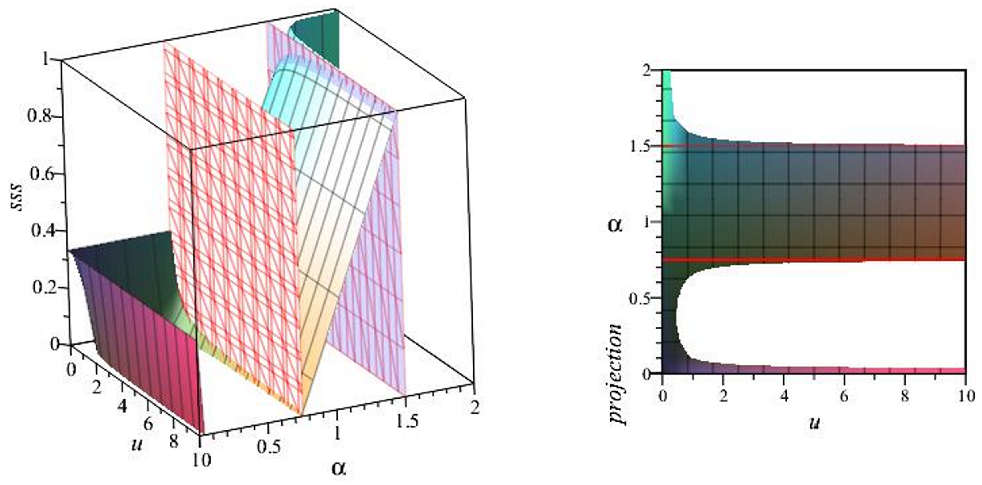
3.1. Power-Law NLED Lagrangian

Magnetic universes have been extensively explored within the framework of NLED theories, often characterized by simple Lagrangian densities. One of the simplest Lagrangians is given by

$$L=-{\displaystyle \frac{1}{4}}F+\alpha F^2,$$

(24)

where the nonlinear term $\propto F^2$ [19,21,23,24,28,29,30] has been suggested to potentially induce a cosmic bounce, thus avoiding the initial singularity known as the Big Bang [23]. On the other hand, Lagrangians featuring inverse powers of the electromagnetic field F are intriguing due to the potential significance of nonlinear electromagnetic effects in both the early and late stages of cosmic evolution. Models employing Lagrangian densities like [14,21,51]

$$L=-{\displaystyle \frac{1}{4}}F-{\displaystyle \frac{\gamma }{F}},$$

(25)

have been proposed to elucidate the late-time accelerated expansion of MUs [14]. Additionally, combinations of positive and negative powers of F have been investigated [21,51,56], as exemplified by

$$L=-{\displaystyle \frac{1}{4}}F-{\displaystyle \frac{\gamma }{F}}+\alpha F^2.$$

(26)

This composite model captures key cosmic evolutionary stages and remarkably avoids the cosmological Big Bang singularity. Specifically, the quadratic term $\propto F^2$ dominates during early epochs, facilitating a nonsingular bounce, while the Maxwell term $\propto -F$ takes precedence in the radiation era. At late times, the term $\propto F^{-1}$ governs, driving cosmic acceleration [51].

In [21], it was demonstrated that numerous cosmological models rooted in NLED Lagrangians (24)–(26) are susceptible to curvature singularities of sudden and/or big rip varieties, or exhibit pronounced instability against minor perturbations of the cosmological background—often attributed to the negative sign of SSS. Moreover, concerns regarding causality may emerge due to the potential superluminal propagation of background perturbations.

The subsequent extension of the Lagrangian density involves incorporating a power-law dependence on the invariant F, expressed as

$$L=-\gamma F^{\alpha }.$$

(27)

In this scenario, upon evaluating the SSS Equation (18), we find $c_s^2=-1+{\displaystyle \frac{4}{3}}\alpha$. It becomes evident that the Lagrangian density of NLED remains causal and stable within the range of $\alpha$ values spanning $3/4\le \alpha \le 3/2$.

Now, let us examine the Lagrangian density of NLED expressed as

$$L=-{\displaystyle \frac{1}{4}}F-\gamma F^{\alpha }.$$

(28)

This model characterizes a universe featuring linear Maxwell radiation alongside a nonlinear power-law term. A prior investigation [21] explored specific cases of $\alpha$ ($\alpha =-1$ and $\alpha =2$), revealing that these models fail to meet the necessary constraints for SSS. In [57], the authors examined a variant incorporating cold dark matter (${\rho }_m$ with $p_m=0$). Their analysis, anchored in astronomical observations and with $\gamma <0$, demonstrated that the Lagrangian (28) accurately replicates dark energy phenomena for $\alpha =-1/4$ and $\alpha =-1/8$. More recently, Ref. [58] explored a cosmological framework involving a variable Newton’s constant, $G(t)$, alongside an NLED of the form $L=-{\displaystyle \frac{F^{\alpha }}{4}}$. They established its stability within the range $7/4\le \alpha \le 5/2$.

The expression for the SSS Equation (18), corresponding to the Lagrangian (28) in terms of the scale factor a and the parameter $\alpha$, reads

$$c_s^2={\displaystyle \frac{1}{3}}+{\displaystyle \frac{16\alpha (\alpha -1)\gamma F^{\alpha }}{12\alpha \gamma F^{\alpha }+3F}}={\displaystyle \frac{1}{3}}+{\displaystyle \frac{16\alpha (\alpha -1)\gamma F_0^{\alpha -1}{a}^{4(1-\alpha )}}{12\alpha \gamma F_0^{\alpha -1}{a}^{4(1-\alpha )}+3}},$$

(29)

where on the right-hand side of this equation we have used the solution to the equation of the conservation of the electromagnetic field (9): $F=F_0{a}^{-4}$.

The plot of the SSS (29) in the right panel of Figure 1 shows that the model (28) remains stable and causal within a narrow range of $\alpha$ values, specifically $3/4\le \alpha \le 3/2$. In [57], the NLED Lagrangian (28) was considered, and for the obtained values of $\alpha$, namely, $\alpha =-1/4$ and $\alpha =-1/8$), the resulting SSSs are $c_s^2=-4/3$ and $c_s^2=-7/6$, respectively, indicating gradient instability. Similarly, the cases with $\alpha =-1$ and $\alpha =2$, as shown in [21], yield $c_s^2=-7/3$ and $c_s^2=5/3$, respectively, reaffirming the gradient and also tachyon instabilities in these models.

We have already commented on the fact that for NLED-based models like the one given by the Lagrangian (28) a change in sign of the statefinder parameter s is correlated with a change in sign of the squared speed of sound $c_s^2$. In the present case,

$$s=c_s^2{\displaystyle \frac{4F{L}_{,F}}{4F{L}_{,F}-3L}}=4c_s^2{\displaystyle \frac{1+4\alpha \gamma F_0^{\alpha -1}{a}^{4(1-\alpha )}}{1-4(3-4\alpha )\gamma F_0^{\alpha -1}{a}^{4(1-\alpha )}}},$$

(30)

where $c_s^2$ is given by (29). It can be seen that for $\alpha >3/4$, since $c_s^2\ge 0$ during the course of the cosmic evolution, and the ratio $R\equiv 4F{L}_{,F}/(4F{L}_{,F}-3L)$ is a positive-valued function as well, the statefinder parameter s does not change sign. In general, for non-negative $\alpha$-s, this parameter does not change sign. However, for negative $\alpha <0$, we have the following picture. At very early times ($a\to 0$), $c_s^2=1/3>0$ and the ratio $R=4>0$, while at late times ($a\to \infty$), $c_s^2=4\alpha /3-1<0$ and $R=4\alpha /(4\alpha -3)>0$. This means that for $\alpha <0$, the statefinder parameter $s=c_s^{2}R$ changes sign from $s>0$ to $s<0$ during cosmic expansion. When $s>0$, the expansion is more similar to models like a quintessence, where the present accelerated expansion of the universe is explained as being due to a form of dark energy different from a cosmological constant. However, when $s<0$, the expansion suggests models that could be more similar to those with phantom energy or other exotic forms of energy.

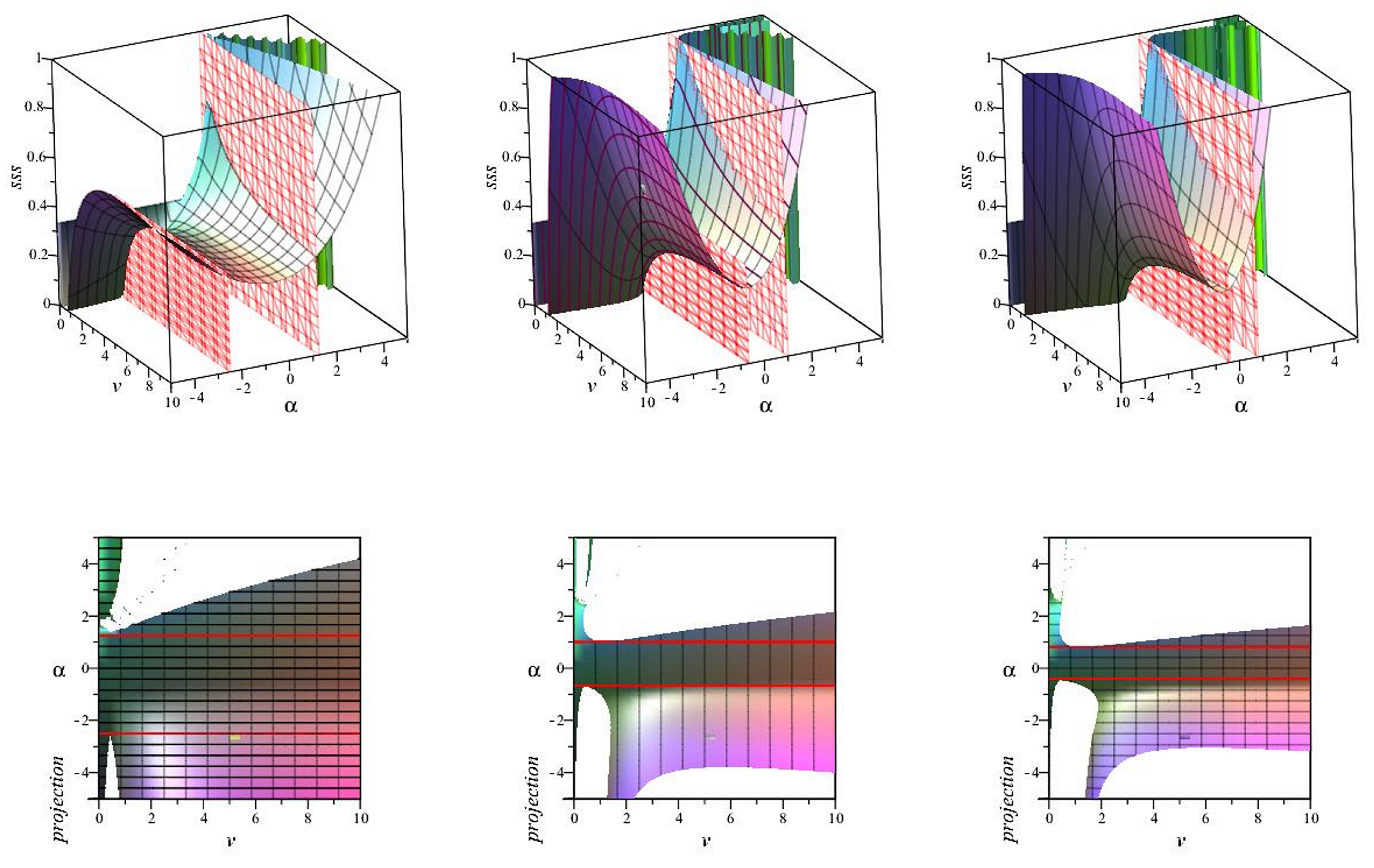
3.2. Generalized Rational Nonlinear Electrodynamics

In this section, we explore a generalized model of NLED described by the following Lagrangian density:

$$L=-{\displaystyle \frac{F}{4}}-{\displaystyle \frac{bF}{1+ϵ{(2ϵ\beta F)}^{\alpha }}},$$

(31)

where b, $ϵ=\pm 1$ and $\alpha$ are dimensionless parameters, and $\beta$ is a parameter with dimensions ${[L]}^4$. To ensure that the Lagrangian remains real, in [59] is stated that $ϵ=1$ for $B>E$ and $ϵ=-1$ for $B<E$. However, in our case, since $E=0$, we only consider the scenario where $ϵ=1$. We recover Maxwell’s electrodynamics when $b=0$. Furthermore, when we apply the weak field approximation ($\beta F\ll 1$), the power series expansion of L (Equation (31)) reveals that nonlinearity persists. This implies the existence of nonlinearity even at late times, which is important for exploring its implications for the model’s behavior during those periods, providing this Lagrangian density proves to be stable and causal.

Some particular cases of the Lagrangian density (31) have been previously analyzed in various studies [31,60,61,62,63,64], primarily investigating black hole solutions with different values of $\alpha$, particularly when $\alpha =1/2$, and for both values of $ϵ$. In [59], it was demonstrated that singularities of point electric charges are absent, and the electromagnetic energy is finite.

The expression for the SSS corresponding to the Lagrangian (31) in terms of the scale factor a and the parameters $\alpha$, $\beta$, and b, is as follows:

$$\begin{array}{ccc}\hfill c_s^2& =& {\displaystyle \frac{1}{3}}-{\displaystyle \frac{16}{3}}{\displaystyle \frac{b\alpha \left[(\alpha -1){(2\beta F)}^{2\alpha }-(\alpha +1){(2\beta F)}^{\alpha }\right]}{(1+{(2\beta F)}^{\alpha })\left[(2-4b(\alpha -1)){(2\beta F)}^{\alpha }+{(2\beta F)}^{2\alpha }+4b+1\right]}}\hfill \\ & =& {\displaystyle \frac{1}{3}}+{\displaystyle \frac{16b\alpha v\left[1-\alpha +(1+\alpha )v\right]}{3(1+v)\left[1+2kv+(1+4b)v^2\right]}},\hfill \end{array}$$

(32)

where we have defined the constant $k\equiv 1+2b(1-\alpha )$ and we have used the compact notation $v\equiv {(a^4/2\beta F_0)}^{\alpha }.$ If we assume that the constants $\beta$ and b are non-negative reals, a pure qualitative analysis complemented with the numerical study (see Figure 2) reveals that there is always a non-empty range of $\alpha$ values where the model is free of instability against small perturbations of the background and also of tachyon instability, i.e., where SSS meets the bounds $0\le c_s^2\le 1$, at all stages of the cosmic expansion. For instance, if we take $b=1$, for $-2/3\le \alpha \le 1$, the model is both causal and stable. The width of the $\alpha$—range depends on the constant b: For larger values of the constant b the range is wider.

Generalized Rational Nonlinear Electrodynamics without Maxwell Term

Let us examine in more detail a generalized model of rational nonlinear electrodynamics [59], excluding the linear Maxwell term and focusing on magnetic universes, described by the following Lagrangian density ($ϵ=1$):

$$L=-{\displaystyle \frac{bF}{1+{(2\beta F)}^{\alpha }}},$$

(33)

For the limit $\beta \to 0$, the Lagrangian (33) reduces to Maxwell’s theory. Specific cases of this Lagrangian density have been studied in the cosmological context [59,60], detailed in [31,32,33,34,65]. A very special case of the Lagrangian density (33) where $\alpha =1$ has been studied in [31,32,33,60,66].

The squared sound speed for the Lagrangian density (33) is given by

$$c_s^2={\displaystyle \frac{1}{3}}-{\displaystyle \frac{4}{3}}{\displaystyle \frac{\alpha [(\alpha -1){(2\beta F)}^{2\alpha }-{(2\beta F)}^{\alpha }(1+\alpha )]}{[1+{(2\beta F)}^{\alpha }][(\alpha -1){(2\beta F)}^{\alpha }-1]}}={\displaystyle \frac{1}{3}}-{\displaystyle \frac{4\alpha \left[1-\alpha +(1+\alpha )v\right]}{3(1+v)(1-\alpha +v)}},$$

(34)

where, as before, $v\equiv {(a^4/2\beta F_0)}^{\alpha }$. A straightforward inspection of (34) shows that, for $-1/2\le \alpha \le 1/4$, the model (33) is stable against small perturbations of the background and is free of tachyonic instability as well (see Figure 3). As seen in Figure, in the region over the surface $c_s^2=c_s^2(v,\alpha )$ (34), lying between the vertical planes at $\alpha =-1/2$ and $\alpha =1/4$, the squared speed of sound meets the bounds $0\le c_s^2\le 1,$ within which the model is both causal and stable.

The equations of motion of the model (33) are complex enough to warrant further investigation through a dynamical systems analysis, particularly within the parameter range $-1/2\le \alpha \le 1/4$, where no issues with instability against small perturbations of the background or with tachyon instability arise.

Recently, in [65], the dynamics of this model have been analyzed. However, the stability and causality analysis in that work were verified only for values which fall outside of the range $-1/2\le \alpha \le 1/4$. Therefore, in our work, we can perform a more comprehensive dynamical analysis within the parameter space we have identified as stable and causal. From the above, we can infer a specific region in the parameter space for the Lagrangian (33), where a dynamical analysis can be conducted in a homogeneous and isotropic framework to observe its effects during early and late times.

4. Dynamical Systems Analysis of Models with Stable and Causal Lagrangian Density

In this section, we perform a dynamical analysis of models where nonlinear radiation is stable and causal. Given the complexity of the equations of motion, here we utilize the tools provided by dynamical systems theory for this. These tools allow one to inspect the global (asymptotic) dynamics of cosmological models in some auxiliary phase space where the equilibrium asymptotic configurations amount to those solutions which are preferred by the system of differential equations of the cosmological model under study [67]. Attractor solutions represent those cosmological stages which the system naturally evolves to in the asymptotic future. Meanwhile, source critical points represent those asymptotic cosmological stages in the past from where the system evolves into the future. In particular, if past attractors exist, these mark the points in the phase space in whose neighborhood the initial conditions are to be given. Transient stages of the cosmic evolution such as, for instance, primordial inflation and matter dominance, are associated with saddle equilibrium points. Our task is to determine whether there are past and future attractors, as well as saddle critical points, in the phase space of the cosmological models under study.

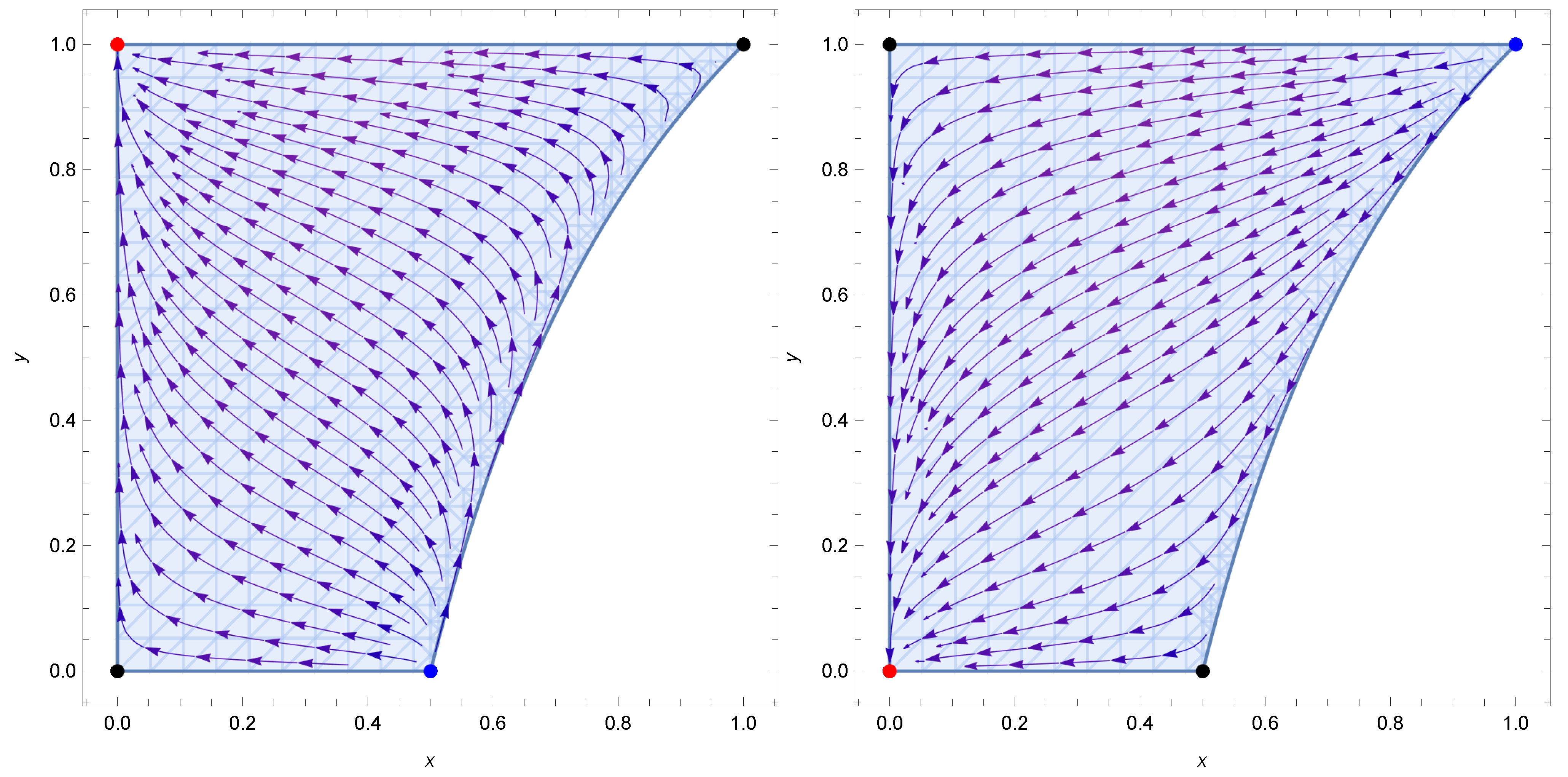
4.1. Power-Law Lagrangian

In the previous section, we found that a power-law model of nonlinear electrodynamics (28) is stable and causal as long as $3/4\le \alpha \le 3/2$. We now analyze the evolution of a homogeneous and isotropic model whose matter content is given by this NLED and ordinary matter (cold dark matter). Thus, if we take the density for ordinary matter as ${\rho }_m$ (considering non-relativistic dust (${\omega }_m=0$) and the nonlinear electromagnetic field given by the Lagrangian (28), the dynamical equations to study are the following (8):

$$\begin{array}{ccc}& & 3H^2={\rho }_m+{\displaystyle \frac{F}{4}}+\gamma F^{\alpha },-2\dot{H}={\rho }_m+{\displaystyle \frac{1}{3}}F+{\displaystyle \frac{4}{3}}\gamma \alpha F^{\alpha },\hfill \\ & & {\dot{\rho }}_m=-3H{\rho }_m(1+{\omega }_m),\dot{F}=-4HF.\hfill \end{array}$$

(35)

Dynamical systems theory requires the transformation of this second-order system into a first-order system by going into an auxiliary phase space spanned by the variables [67]

$$x={\displaystyle \frac{F}{12H^2}}={\Omega }_{\mathrm{rad}},y=\gamma {\displaystyle \frac{F^{\alpha }}{3H^2}}={\Omega }_{\mathrm{rad}}^{\mathrm{nled}},$$

(36)

Thus, the first of Equations (35) can be written as ${\Omega }_m+{\Omega }_{\mathrm{rad}}+{\Omega }_{\mathrm{rad}}^{\mathrm{nled}}=1$, or equivalently,

$${\Omega }_m=1-x-y,$$

(37)

where we see that the variables are bounded within the phase space

$$\Psi =\{(x,y)|0\le x+y\le 1,0\le x\le 1,0\le y\le 1\}.$$

(38)

The second Equation (35) takes the form

$$-2{\displaystyle \frac{\dot{H}}{H^2}}=3{\Omega }_m+4x+4\alpha y=3+x+(4\alpha -3)y.$$

(39)

The dynamical system reads

$$\begin{array}{ccc}\hfill x^{\prime }& =& -2x\left(2+{\displaystyle \frac{\dot{H}}{H^2}}\right)=x[x-1+(4\alpha -3)y],\hfill \\ \hfill y^{\prime }& =& -2y\left(2\alpha +{\displaystyle \frac{\dot{H}}{H^2}}\right)=y[(4\alpha -3)y+x+3-4\alpha ],\hfill \end{array}$$

(40)

where the prime denotes the derivative with respect to $\tau$, which is the conformal time, $\tau =\int {\displaystyle \frac{dt}{a(t)}}$. In terms of the variables (36) of the phase space, the squared sound speed (29) can be written as

$$c_s^2={\displaystyle \frac{x+\alpha (4\alpha -3)y}{3(x+\alpha y)}}.$$

(41)

Finally, both the effective barotropic parameter, ${\omega }_{eff}$, in Equation (13) and the deceleration parameter q in Equation (16) in the new variables are given by

$${\omega }_{eff}={\displaystyle \frac{1}{3}}x+{\displaystyle \frac{4\alpha -3}{3}}y,q={\displaystyle \frac{1}{2}}\left[1+x+(4\alpha -3)y\right]$$

(42)

and the statefinder parameters are given by

$$r=1+2x+2\alpha (4\alpha -3)y,s={\displaystyle \frac{4[x+\alpha (4\alpha -3)y]}{3[3x+(4\alpha -1)y]}}.$$

(43)

The critical points of the dynamical system (40) within the phase space $\Psi$ (38) are the following:

• At the first critical point, $P_m(0,0)$, ordinary matter dominates (${\Omega }_m=1$). The behavior of this critical point, as determined by the eigenvalues ${\lambda }_1=-1$ and ${\lambda }_2=3-4\alpha$, indicates that it is a decelerated ($q=1/2$) future attractor when $\alpha >3/4$ ($c_s^2$-stable) and a saddle point when $\alpha <3/4$ ($c_s^2$-unstable). The effective barotropic parameter ${\omega }_{\mathrm{eff}}=0$ indicates that the combined effect of ordinary matter and nonlinear radiation is such that the expansion of the universe behaves as if it is dominated by non-relativistic matter. This is consistent with a dust-dominated universe within the framework of standard cosmology. Finally, the statefinder parameters take the values $r=1$ and $s=$ undefined. This indicates that the cosmological model exhibits characteristics of the $\Lambda$CDM model with respect to the parameter r. However, the parameter s is undefined, so that there must be appreciable deviations from the $\Lambda$CDM model. This reflects the influence of the nonlinear electrodynamics on the universe’s dynamics, distinguishing it from a purely matter-dominated model.
• The second point $P_{\mathrm{rad}}(1,0)$, where Maxwell radiation dominates with ${\Omega }_{\mathrm{rad}}=1$ and $c_s^2={\displaystyle \frac{1}{3}}$, has eigenvalues ${\lambda }_1=1$ and ${\lambda }_2=4-4\alpha$. This indicates that it is a decelerated ($q=1$) source (past attractor) when $\alpha <1$ and a saddle point when $\alpha >1$. An effective EOS parameter ${\omega }_{eff}=1/3$ indicates that the combined effect of ordinary matter and nonlinear radiation results in the expansion of the universe behaving as if it were dominated by radiation. The statefinder parameters take the values $r=3$ and $s=4/9$. These values indicate significant deviations from the $\Lambda$CDM model. These deviations reflect the nonlinear electrodynamics’ impact on the dynamics of the universe.
• For the point $P_{\mathrm{rad}}^{\mathrm{nled}}(0,1)$, where nonlinear radiation dominates ${\Omega }_{\mathrm{rad}}^{\mathrm{nled}}=1$, the squared sound speed is given by $c_s^2=(4\alpha -3)/3$. The eigenvalues ${\lambda }_1=4\alpha -3$ and ${\lambda }_2=4(\alpha -1)$ indicate that this point is a future attractor if $\alpha <3/4$ ($c_s^2$-unstable), a saddle point if $3/4<\alpha <1$ ($c_s^2$-stable), and a source (past attractor) if $\alpha \ge 1$ ($c_s^2$-stable if $\alpha \le 3/2$). The deceleration parameter at this point is $q=2\alpha -1$, which indicates an accelerated expansion if $\alpha <{\displaystyle \frac{1}{2}}$; however, this value of the $\alpha$-parameter falls outside of the range where the model is stable and causal. For $\alpha >{\displaystyle \frac{1}{2}}$ the expansion is always decelerated. The effective EOS parameter ${\omega }_{eff}=-1+4\alpha /3$. The statefinder parameters for this critical point take the values $r=1+2\alpha (4\alpha -3)$ and $s=4\alpha (4\alpha -3)/3(4\alpha -1)$. The dependence of the statefinder parameters on $\alpha$ reflects the impact of nonlinear electrodynamics on the dynamics of the universe, providing insights into appreciable deviations from the $\Lambda$CDM model.

The evolution of the model can be divided into three scenarios depending on the value of the parameter $\alpha$:

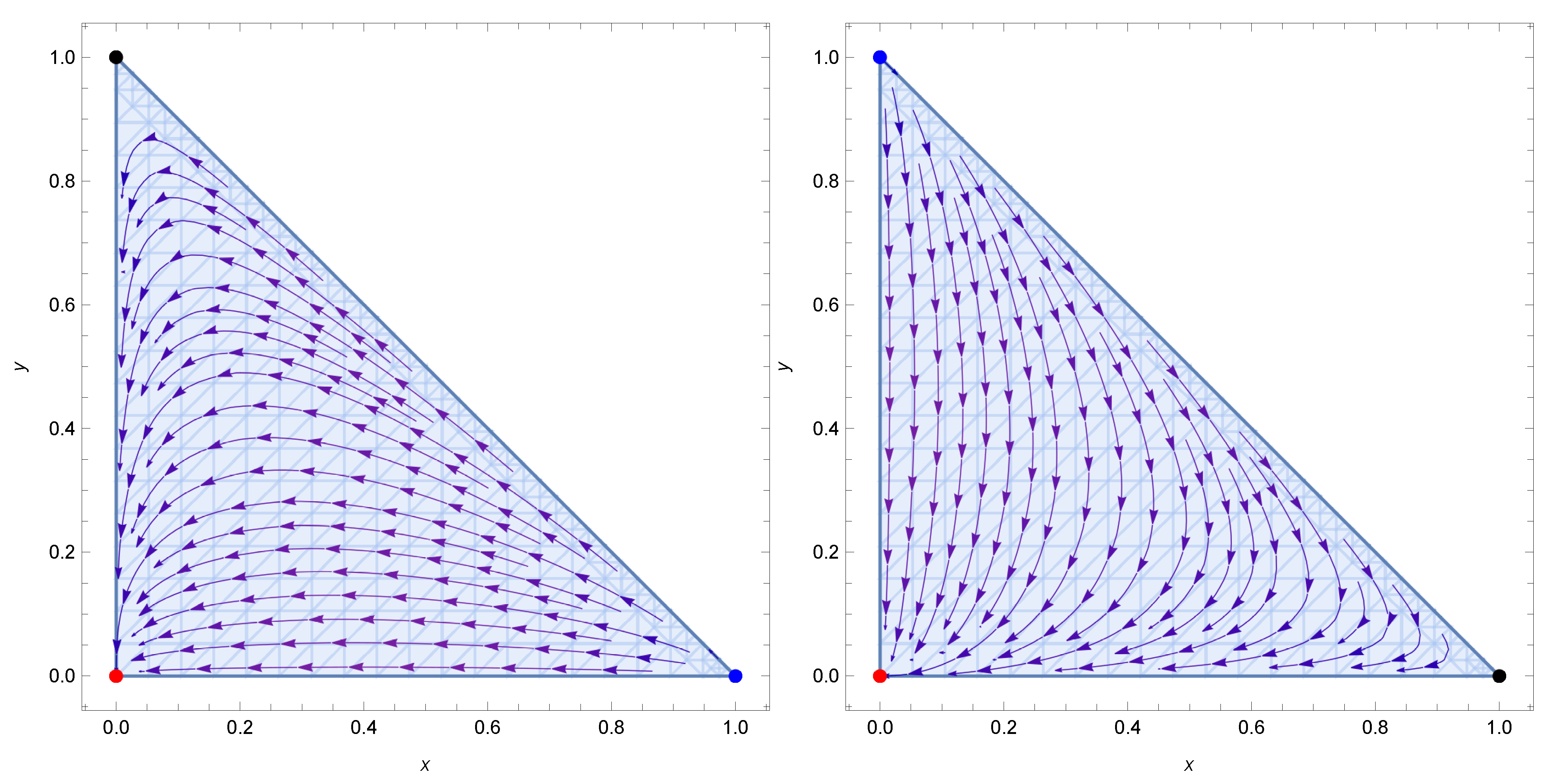
• For $\alpha <3/4$ the dynamics of the model start from a Maxwell radiation domain ($P_{\mathrm{rad}}$), transiently approach the matter-dominated phase ($P_m$), and are finally attracted towards the nonlinear radiation domain ($P_{\mathrm{rad}}^{\mathrm{nled}}$). The transient matter-dominated stage could explain the correct amount of structure formation. In the case when $\alpha <1/2$, the attractor solution depicts accelerated expansion, so that the nonlinear radiation could explain the accelerated expansion of the universe without the need for any dark energy. Unfortunately, this scenario is not physically acceptable because the values of the parameter $\alpha$ fall outside of the range $3/4\le \alpha \le 3/2$, where the model is free of gradient and tachyon instabilities.
• For $3/4\le \alpha <1$, all trajectories start from the Maxwell radiation-dominated point ($P_{\mathrm{rad}}$), then these approach to a transient stage where the nonlinear radiation dominates ($P_{\mathrm{rad}}^{\mathrm{nled}}$), and eventually, reach the matter-dominated attractor ($P_m$). The values of the statefinder parameters vary from one critical point to another. This means that the model exhibits a dynamic behavior quite distinct from the standard cosmological model, indicating that the influence of nonlinear electrodynamics introduces substantial differences in the evolution of the universe compared to a $\Lambda$CDM framework, see the left panel of the Figure 4.
• For $1<\alpha <3/2$, the orbits in the phase space are sourced by the nonlinear radiation ($P_{\mathrm{rad}}^{\mathrm{nled}}$), evolve transiently near the Maxwell radiation-dominated point ($P_{\mathrm{rad}}$), and are finally attracted towards the matter-dominated point ($P_m$). The values of the statefinder parameters change from critical point to critical point, for instance, at the past attractor

  $$r=1+2\alpha (4\alpha -3),s={\displaystyle \frac{4\alpha (4\alpha -3)}{3(4\alpha -1)}},$$

  while at the future attractor $r=1$, $s=$ undefined, and at the Maxwell point ($P_{\mathrm{rad}}$) $r=3$ and $s=4/9$. These values do not closely align with the consensus $\Lambda$CDM model, signaling appreciable departures from it, see the right panel of the Figure 4.

In this section, we have analyzed the dynamic evolution of a nonlinear power-law model of electrodynamics characterized by the Lagrangian density (28). Previously, we have demonstrated that this model is stable and causal within the parameter range $3/4\le \alpha \le 3/2$. The dynamics of this model exhibit two relevant scenarios: In the first scenario, the model starts in a Maxwell radiation-dominated state, transitions through a transient phase dominated by nonlinear radiation, and ultimately culminates in a matter-dominated state. In the second scenario, the model begins in a nonlinear radiation-dominated state, transiently passes through a Maxwell radiation-dominated phase, and finally, reaches a matter-dominated state. These results provide a comprehensive understanding of the dynamic evolution and stability of the nonlinear power-law electrodynamics model. Furthermore, the statefinder analysis reveals that while the model’s parameters do not align closely with the $\Lambda$CDM model, they still offer valuable insights into the deviations introduced by nonlinear electrodynamics. Specifically, the statefinder parameters help quantify how much the model diverges from the standard cosmological model, highlighting the unique NLED effects on the evolution of the universe.

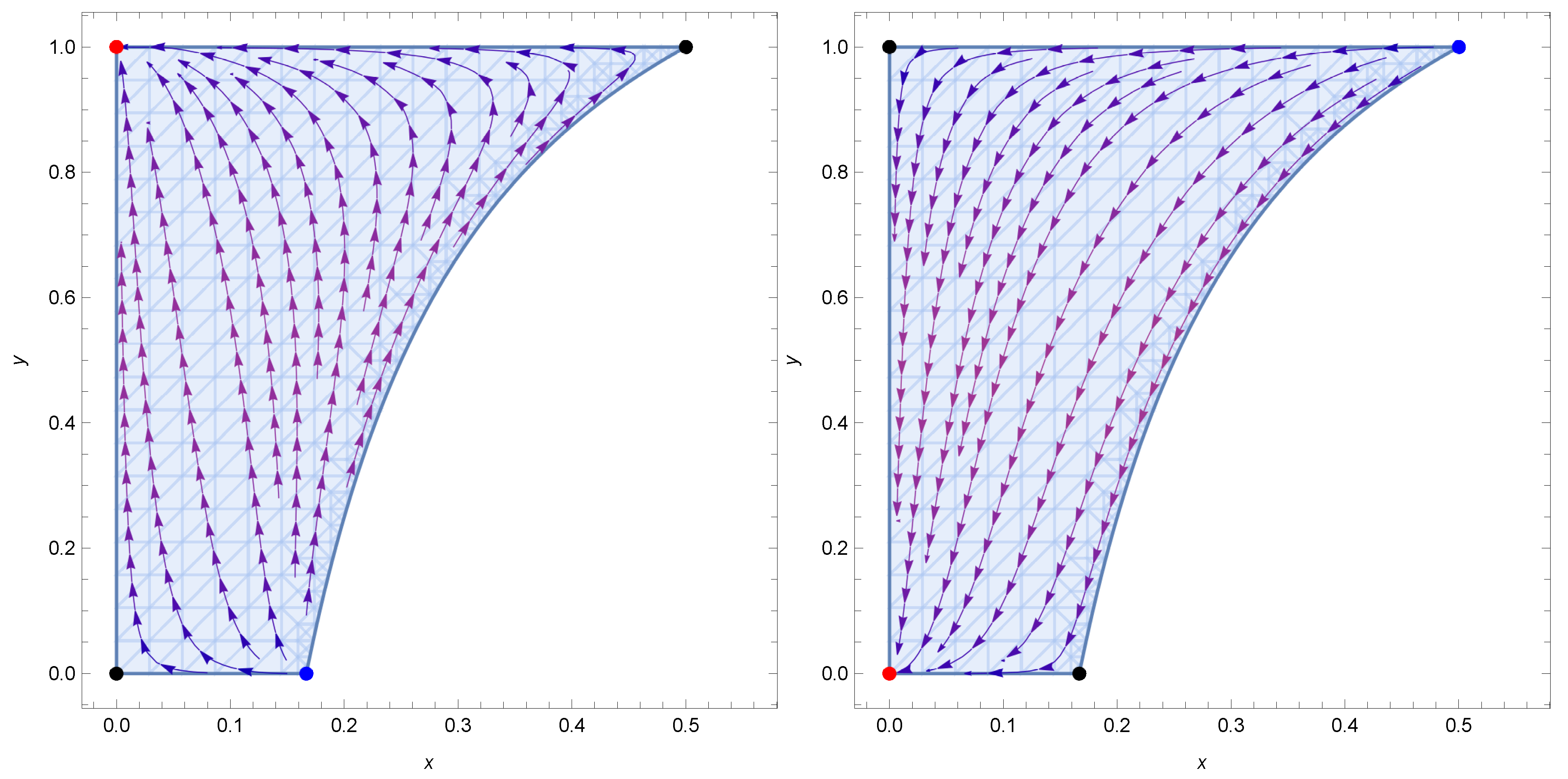
4.2. Generalized Rational Nonlinear Electrodynamics Dynamical Evolution without Maxwell Term

The next model we will analyze using dynamical systems corresponds to the Lagrangian density given by (33), which we have demonstrated to be causal and stable for the range $-1/2\le \alpha \le 1/4$. The dynamical equations for this model are given by

$$3H^2={\rho }_m+{\displaystyle \frac{bF}{1+{(2\beta F)}^{\alpha }}},-2\dot{H}={\rho }_m-{\displaystyle \frac{4bF}{3}}\left[{\displaystyle \frac{(\alpha -1){(2\beta F)}^{\alpha }-1}{{(1+{(2\beta F)}^{\alpha })}^2}}\right],$$

(44)

and $\dot{F}=-4HF$. Here, we consider ordinary (pressureless) matter ${\rho }_m$ ($p_m=0$).

We consider the following new bounded phase plane variables to obtain an autonomous first-order dynamical system:

$$x={\displaystyle \frac{bF}{bF+3H^2}},y={\displaystyle \frac{{(2\beta F)}^{\alpha }}{1+{(2\beta F)}^{\alpha }}}.$$

(45)

Thus, Equations (46) in these new variables can be expressed as

$${\Omega }_m=1-{\Omega }_{\mathrm{rad}}^{\mathrm{nled}}=1-{\displaystyle \frac{x(1-y)}{1-x}},-2{\displaystyle \frac{\dot{H}}{H^2}}=3{\Omega }_m+{\displaystyle \frac{4x(1-y)(1-\alpha y)}{1-x}},$$

(46)

where

$${\Omega }_m={\displaystyle \frac{{\rho }_m}{3H^2}},{\Omega }_{\mathrm{rad}}^{\mathrm{nled}}={\displaystyle \frac{bF/3H^2}{1+{(2\beta F)}^{\alpha }}}.$$

The deceleration parameter, effective equation of state (EOS) parameter, and the SSS (34) are given by

$$\begin{array}{ccc}& & q={\displaystyle \frac{1-x+x(1-y)(1-4\alpha y)}{2(1-x)}},{\omega }_{eff}=-{\displaystyle \frac{x(1-y)(1-4\alpha y)}{3(1-x)}},\hfill \\ & & c_s^2={\displaystyle \frac{1}{3}}-{\displaystyle \frac{4\alpha y(1+\alpha -2\alpha y)}{3(1-\alpha y)}},\hfill \end{array}$$

respectively, while the statefinder parameters read

$$r=1+{\displaystyle \frac{2x(1-y)[1-(5+4\alpha )\alpha y+8{\alpha }^2{y}^2]}{1-x}},s={\displaystyle \frac{4[1-(5+4\alpha )\alpha y+8{\alpha }^2{y}^2]}{3(1-4\alpha y)}}.$$

The 2D dynamical system for this model reads

$$x^{\prime }=-2x(1-x)\left(2+{\displaystyle \frac{\dot{H}}{H^2}}\right),y^{\prime }=-4\alpha y(1-y),$$

(47)

where the prime denotes differentiation with respect to $\tau =lna$. The phase space in which to look for equilibrium configurations of the dynamical system (47) is defined by

$$\Psi =\left\{(x,y)\left|0\le x\le 1,0\le y\le 1,y\ge {\displaystyle \frac{2x-1}{x}}\right\},\right.$$

(48)

where the lower bound on the variable y comes from requiring that ${\Omega }_m\ge 0.$

Below, we show the critical points of the dynamical system (47). We include the values of several cosmological parameters of observational significance evaluated at the critical points:

• The first critical point, $P_m(0,0)$, dominated by ordinary matter (${\Omega }_m=1$), is decelerated ($q={\displaystyle \frac{1}{2}}$), and its effective barotropic parameter simulates dust (${\omega }_{eff}=0$). At this point, the SSS corresponds to Maxwell radiation, meaning $c_s^2={\displaystyle \frac{1}{3}}$. The Jacobian matrix’s eigenvalues are ${\lambda }_1=-1$ and ${\lambda }_2=-4\alpha$. This indicates that $P_1$ is a future attractor if $\alpha >0$ and a saddle point if $\alpha <0$. The values of the statefinder parameters at this point are both positive: $r=1$ and $s=4/3$. The significant deviation of s from zero indicates a considerable divergence from the standard cosmological model. This substantial positive value of s reflects a significant influence of nonlinear electrodynamics on the universe’s dynamics.
• The point $P_M(0,1)$ corresponds to decelerated expansion as well ($q=1/2$), and it is also dominated by ordinary matter. The effective EOS parameter ${\omega }_{eff}=0$ means that the background fluid mimics dust. The SSS at this point is given by $c_s^2=(1-4\alpha )/3.$ Therefore, the stability and causality depend on the value of $\alpha$, which must satisfy the condition found in the previous section: $-1/2\le \alpha \le 1/4$. The eigenvalues of the Jacobian matrix are ${\lambda }_1=-1$ and ${\lambda }_2=4\alpha$, indicating that $P_2$ is a future attractor if $\alpha <0$ and a saddle point otherwise. The values of the statefinder parameters for this point are given by $r=1$ and $s=4(1-\alpha )/3$. The parameter s varies with $\alpha$, indicating how the nonlinear electrodynamics affects the model’s deviation from the standard cosmological model. Specifically, the expression for s highlights the sensitivity of the model’s behavior to the parameter $\alpha$. Only when $\alpha =1$ does the model exhibit behavior similar to $\Lambda$CDM, where $s=0$.
• The point $P_{\mathrm{rad}}\left(1/2,0\right)$ is dominated by Maxwell radiation (${\omega }_{eff}=1/3$), with

  $${\Omega }_{\mathrm{rad}}={\displaystyle \frac{bF}{12H^2}}={\displaystyle \frac{x}{1-x}}=1,$$

  and represents decelerated expansion ($q=1$). The SSS $c_s^2=1/3$. The eigenvalues of the Jacobian matrix at this point are ${\lambda }_1=1$ and ${\lambda }_2=-4\alpha$, indicating that this point acts as a past attractor if $\alpha <0$ and as a saddle point for other values. For the statefinder parameters, we obtain that $r=3$ and $s=4/3$. These values imply that the cosmological model at this critical point behaves very differently from the $\Lambda$CDM model.
• For the critical point $P_{\mathrm{rad}}^{\mathrm{nled}}=(1,1)$, several of the relevant cosmological parameters such as ${\Omega }_m,$$q,$${\omega }_{eff},$ and the statefinder parameter r, are undefined. The only parameters which one can determine are $c_s^2=(1-4\alpha )/3$ and $s=4(1-\alpha )/3$. The eigenvalues of the Jacobian matrix at this point are ${\lambda }_1=1$ and ${\lambda }_2=4\alpha$, indicating that it acts as a past attractor if $\alpha >0$, otherwise it is a saddle point. These features of the NLED-based equilibrium configuration suggests that the nonlinear effects of the magnetic field play an important role in the course of cosmic expansion.

The features of the cosmological model (33) are illustrated in Figure 5 for two distinct values of the parameter $\alpha$ which fall within the range $-1/2\le \alpha \le 1/4$, where the model is free of gradient and tachyon instabilities: $\alpha =-0.1$ and $\alpha =0.1$, respectively. Regardless of the specific value of $\alpha$, the phase space consistently displays a past attractor (blue point), a saddle point (black point), and a future attractor (red point). This structure indicates that the initial conditions should be set near those of the past attractor, from which the orbits of the dynamical system move towards the saddle point—representing a transient phase in cosmic evolution—before converging on the future attractor. The primary effect of the parameter $\alpha$ is to determine the roles of the different asymptotic states, interchanging their positions as past or future attractors and the saddle point configuration.

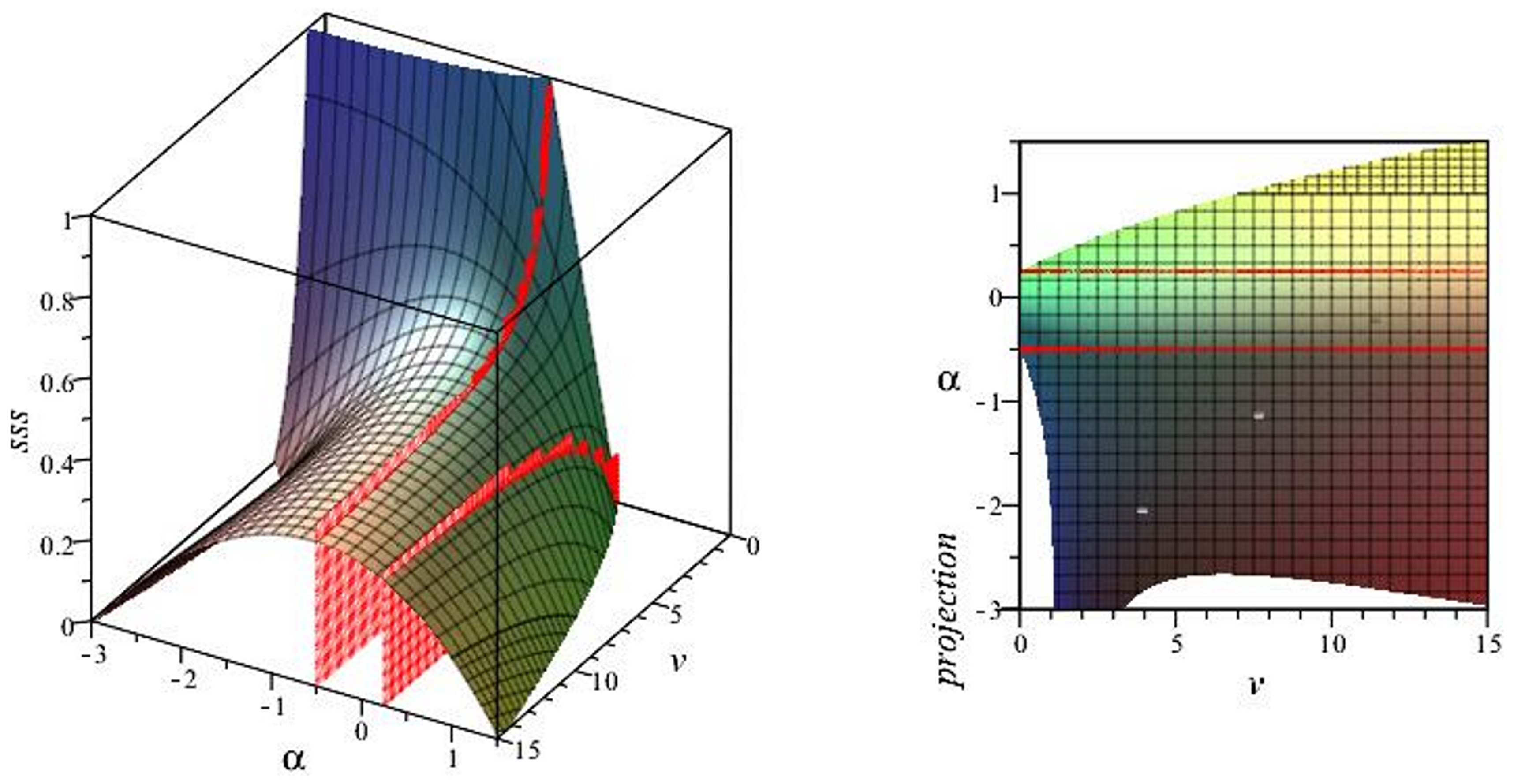
4.3. Generalized Rational Nonlinear Electrodynamics Dynamical Evolution with Maxwell Term

In this section, we analyze the dynamical evolution of a model corresponding to the Lagrangian density given by (31) with $ϵ=1$. Finding exact solutions of the equations of motion of this model is a complex task, and even if we find several exact cosmological solutions, these may belong in a set of measure zero. This is why in this and in the other cases in this paper we apply the tools of dynamical systems theory. Our task is to search for the critical points of the resulting dynamical system in some auxiliary phase space. These equilibrium configurations amount to those solutions of the original system of cosmological equations which are generic, and so, are the most relevant ones within the infinite set of possible exact solutions.

The dynamical equations for the model (31) are given by

$$\begin{array}{ccc}\hfill 3H^2& =& {\rho }_m+{\displaystyle \frac{F}{4}}+{\displaystyle \frac{bF}{1+{(2\beta F)}^{\alpha }}},\hfill \\ \hfill -2\dot{H}& =& {\rho }_m-{\displaystyle \frac{4F}{3}}\left[-{\displaystyle \frac{1}{4}}-{\displaystyle \frac{b}{(1+{(2\beta F)}^{\alpha })}}+{\displaystyle \frac{b\alpha {(2\beta F)}^{\alpha }}{{(1+{(2\beta F)}^{\alpha })}^2}}\right],\hfill \end{array}$$

(49)

where we are considering ordinary matter ${\rho }_m$ (non-relativistic dust ${\omega }_m=0$) and $\dot{F}=-4HF$.

We consider the following new bounded variables:

$$x={\displaystyle \frac{F}{F+12H^2}},y={\displaystyle \frac{{(2\beta F)}^{\alpha }}{1+{(2\beta F)}^{\alpha }}}.$$

(50)

Thus, the dynamical Equation (49) in these new variables are traded by the following plane-autonomous system of ordinary differential equations:

$$x^{\prime }=-2x(1-x)\left(2+{\displaystyle \frac{\dot{H}}{H^2}}\right),y^{\prime }=-4\alpha y(1-y),$$

(51)

where

$$\begin{array}{ccc}\hfill {\Omega }_m& =& {\displaystyle \frac{{\rho }_m}{3H^2}}=1-{\displaystyle \frac{x[1+4b(1-y)]}{(1-x)}},\hfill \\ \hfill {\displaystyle \frac{\dot{H}}{H^2}}& =& -{\displaystyle \frac{3}{2}}{\Omega }_m-{\displaystyle \frac{2x}{(1-x)}}\left[1+4b(1-y)(1-\alpha y)\right].\hfill \end{array}$$

(52)

The phase space where the physically meaningful critical points of the dynamical system (51) are located is defined by

$$\Psi =\left\{(x,y)\left|0\le x\le 1,0\le y\le 1,{\displaystyle \frac{2x(1+2b)-1}{4bx}}\le y\le {\displaystyle \frac{1+4b}{4b}}\right\}.\right.$$

There are four critical points associated with this dynamical system:

• Matter-dominated critical point $P_m(0,0)$ (${\Omega }_m=1$). At this point the electromagnetic effects are negligible, making this point representative of a purely matter-dominated phase. The deceleration parameter is $q=1/2$, and the effective EOS parameter ${\omega }_{eff}=0$. The squared sound speed is $c_s^2=1/3$, while the statefinder parameters are $r=1$ and $s=(1+4b)/3(1+b)$. The eigenvalues associated with the linearization matrix at this critical point are ${\lambda }_1=-1$ and ${\lambda }_2=-4\alpha$, indicating that this point is a decelerated future attractor if $\alpha >0$ and a saddle point otherwise.
• Second matter-dominated critical point $P_M(0,1)$ (${\Omega }_m=1$). This represents a matter-dominated phase with significant NLED effects, $F\to \infty$. The deceleration parameter is $q=1/2$, the effective EOS parameter ${\omega }_{eff}=0$ and the squared sound speed $c_s^2=1/3$. The statefinder parameters are $r=1$ and $s=1/3$. The eigenvalues associated with this critical point are ${\lambda }_1=-1$ and ${\lambda }_2=4\alpha$, indicating that this point is a saddle point if $\alpha >0$ and decelerated future attractor if $\alpha <0$.
• The critical point $P_{\mathrm{rad}}=(1/2,1)$, with

  $${\Omega }_{\mathrm{rad}}={\displaystyle \frac{F}{12H^2}}={\displaystyle \frac{x}{1-x}}=1,{\Omega }_{\mathrm{rad}}^{\mathrm{nled}}={\displaystyle \frac{bF/3H^2}{1+{(2\beta F)}^{\alpha }}}={\displaystyle \frac{4bx(1-y)}{1-x}}=0,$$

  corresponds to Maxwell radiation domination (the effects of NLED radiation are negligible). This point is characterized by the following values of the relevant cosmological parameters: $q=1$, ${\omega }_{eff}=1/3$, and the squared sound speed $c_s^2={\displaystyle \frac{1}{3}}$. The values of the statefinder parameters are $r=3$ and $s=1/3$. The eigenvalues of the linearization matrix evaluated at this point are ${\lambda }_1=1$ and ${\lambda }_2=4\alpha$, respectively, indicating that this point is a non-accelerated expanding past attractor if $\alpha >0$ and saddle point if not.
• The critical point $P_{\mathrm{rad}}^{\mathrm{nled}}=\left({\displaystyle \frac{1}{2(1+2b)}},0\right)$ is dominated by the combined effect of the nonlinear magnetic and Maxwell radiation fields,

  $${\Omega }_{\mathrm{rad}}={\displaystyle \frac{1}{1+4b}},{\Omega }_{\mathrm{rad}}^{\mathrm{nled}}={\displaystyle \frac{4b}{1+4b}}\Rightarrow {\Omega }_{\mathrm{rad}}+{\Omega }_{\mathrm{rad}}^{\mathrm{nled}}=1.$$

  The point exists for $b\ge -1/4$. The deceleration parameter is $q=1$, the effective EOS parameter ${\omega }_{eff}=1/3$, and the statefinder parameters $r=4$ and $s=(1+4b)/3(1+b)$. The eigenvalues of the linearization matrix are ${\lambda }_1=1$ and ${\lambda }_2=-4\alpha$, respectively, indicating a non-accelerated expanding saddle point if $\alpha >0$ and a past attractor if $\alpha <0$. When $b=0$, this point reduces to the point $P=(1/2,0)$, and when $b\to \infty$, it reduces to the matter-dominant point $P_m=(0,0)$. In the former case, there is not a nonlinear magnetic field, while in the latter case the nonlinear effects decouple from the spectrum of general relativity plus a Maxwell radiation field.

The evolution of the model is graphically depicted in Figure 6 for two different values of the parameter $\alpha$. The left panel illustrates the case when $\alpha =-0.5$, while the right panel corresponds to $\alpha =0.5$.

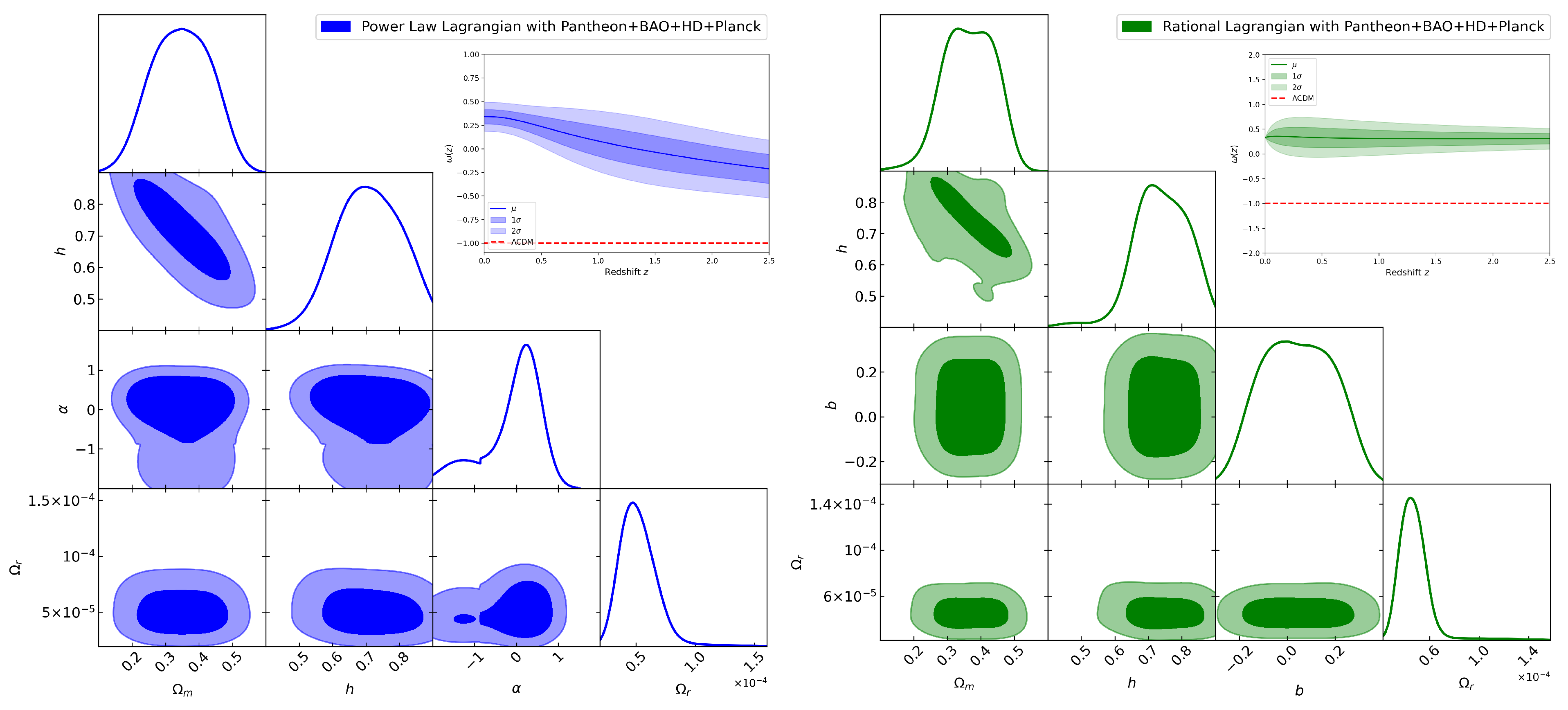
5. Parameter Fitting with Observational Data

Performing parameter fitting using observational data is essential to further validate and refine our models. Parameter fitting allows us to determine the values of the model parameters that best match the empirical data, providing a robust test of the theoretical models against real-world observations. This process is essential for several reasons. Firstly, it enables us to quantify the degree of agreement between the theoretical predictions and the observed data, thus assessing the viability of the models. Secondly, by constraining the parameter values we can reduce the uncertainty in the model predictions, leading to more precise and reliable cosmological insights.

In this study, we use 31 cosmic chronometers collected over several years [68,69,70,71,72,73,74,75]. Additionally, we use high-precision baryon acoustic oscillation (BAO) measurements at different redshifts up to $z<2.36$ from BOSS DR14 quasars (eBOSS) [76], SDSS DR12 Galaxy Consensus [77], Ly-$\alpha$ DR14 cross-correlation [78], Ly-$\alpha$ DR14 auto-correlation [79], the Six-Degree Field Galaxy Survey (6dFGS) [80], and SDSS Main Galaxy Sample (MGS) [81]. In addition, we include SNeIa data from the Pantheon compilation [82] with 1048 supernovae. We also incorporate a compressed version of Planck-15 information, treating the CMB as a BAO experiment at redshift $z=1090$, measuring the angular scale of the sound horizon [83]. These datasets provide a comprehensive and high-precision set of observations that span a significant range of the universe’s history, making them ideal for testing cosmological models incorporating nonlinear electrodynamics (NLED). By fitting the parameters of our NLED models to these observations, we aim to derive constraints that either support or challenge the theoretical framework, ultimately contributing to a deeper understanding of the universe’s evolution.

We employ Bayesian inference to determine the values of the model parameters that best fit the observational data. In this study, we utilize a nested sampling algorithm, using 500 live points, within the library dynesty [84], and the SimpleMC code [85]. The resulting posterior distributions provide constraints on the parameters, enabling us to assess the viability and precision of the NLED models in describing the universe’s evolution. The results of the Bayesian inference are shown in

Table 1. Parameter estimation for the NLED power-law (Equation (53)) and NLED rational (Equation (55)) Lagrangians. The table presents the estimated values of each model’s matter density parameter ${\Omega }_m$, the Hubble parameter h, and the radiation density parameter ${\Omega }_r$. The parameter $\alpha$ is also estimated for the power-law model, while the parameter b is included for the rational model. The $logZ$ values indicate the Bayesian evidence for each model, and the $logB$ values provide the Bayes factor comparison with the $\Lambda$CDM model, showing a strong preference for the $\Lambda$CDM model. The last row qualitatively describes the strength of evidence favoring $\Lambda$CDM over the NLED models.

	Power Law	Rational	$\mathsf{\Lambda }$CDM
${\Omega }_m$	$0.3481\pm 0.0866$	$0.36637\pm 0.0751$	$0.3005\pm 0.0064$
h	$0.7133\pm 0.09745$	$0.7413\pm 0.0829$	$0.6830\pm 0.0049$
${\Omega }_r$	$5.16099\times {10}^{-5}\pm 1.5742\times {10}^{-5}$	$4.7019\times {10}^{-5}\pm 1.3266\times {10}^{-5}$	$5.3018\times {10}^{-5}\pm 7.6633\times {10}^{-7}$
$\alpha$	$-0.0679\pm 0.6644$	–	–
b	–	$0.04566\pm 0.1476$	–
$logZ$	$-1784.16\pm 0.25$	$-2355.57\pm 0.22$	$-538.37\pm 0.215$
$logB$ with $\Lambda$CDM	$1244.8$	$1817.2$	–
Evidence over $\Lambda$CDM	Very strong in favor of $\Lambda$CDM	Very strong in favor of $\Lambda$CDM	–

and in the plots of Figure 7. In Table 1, as a reference, we include the parameter estimation of the $\Lambda$CDM model using the same data and parameters for nested sampling. This allows us, using the logarithm of the Bayesian evidence $logZ$, to calculate the Bayes factor $logB$, and through the Bayes factor and Jeffrey’s scale [86,87], to make a model comparison.

Therefore, we employ Bayesian inference to investigate the parameters of the power-law and rational Lagrangian models, aiming to constrain them using observational data from the late universe. Specifically, we aim to assess whether the nonlinear electrodynamics models are compatible with the available observational evidence and whether the results of our dynamical analysis align with the estimated parameters.

By fitting the parameters of the power-law and rational Lagrangian models to the comprehensive observational datasets, we aim to derive constraints on the model parameters. This approach allows us to evaluate the compatibility of the NLED models with current observational evidence and to determine whether these models can provide a viable description of the universe’s evolution. In addition, we will quantify the degree of agreement between the theoretical predictions of the NLED models and the empirical data. The results of this analysis provide critical insights into the viability and precision of the NLED models in the context of modern cosmology.

In the case of the power-law Lagrangian, the Friedmann Equation (28), useful for performing Bayesian inference, is given by

$${\displaystyle \frac{H^2}{H_0^2}}={\Omega }_{m0}{(1+z)}^{3(1+{\omega }_m)}+{\Omega }_{r0}{(1+z)}^4+{\Omega }_{NL0}{(1+z)}^{4\alpha },$$

(53)

where ${\Omega }_{m0}={\displaystyle \frac{{\rho }_{m0}}{3H_0^2}}$, ${\Omega }_{r0}={\displaystyle \frac{F_0}{12H_0^2}}$, and ${\Omega }_{NL0}=\gamma {\displaystyle \frac{F_0^{\alpha }}{3H_0^2}}$. We use the following flat priors: ${\Omega }_m\in [0.1,0.5]$, $h\in [0.4,0.9]$, and $\alpha \in [-2,2]$.

For the rational Lagrangian,

$$L=-{\displaystyle \frac{F}{4}}-{\displaystyle \frac{bF}{1+2\beta F}},$$

(54)

which is a particular case of (33) for $\alpha =1$; the equation to be used is

$${\displaystyle \frac{H^2}{H_0^2}}={\Omega }_{m0}{(1+z)}^3+{\Omega }_{r0}{(1+z)}^4+4b{\displaystyle \frac{{\Omega }_{r0}{(1+z)}^4}{24\beta H_0^2{\Omega }_{r0}{(1+z)}^4+1}},$$

(55)

where ${\Omega }_{m0}={\displaystyle \frac{{\rho }_{m0}}{3H_0^2}}$ and ${\Omega }_{r0}={\displaystyle \frac{F_0}{12H_0^2}}$. We assume $\beta =1$ and use the flat priors ${\Omega }_m\in [0.1,0.5]$, $h\in [0.4,0.9]$, and $b\in [-27/125,108/343]$ for the Bayesian parameter estimation.

We observe that the datasets used cannot constrain the parameters $\alpha$ and b effectively; however, the values of the matter density ${\Omega }_m$ and the Hubble parameter h for both models are consistent with the expected values for the current universe. The fact that the $\alpha$ and b parameters can take any value within the prior ranges aligns with the results found in the dynamical analysis.

In the triangle plots of Figure 7, the posterior sampling for both Lagrangians and their respective $\omega (z)$ values, using Equation (11) for both cases, can be seen. According to the Bayes factor in Table 1, the $\Lambda$CDM model is significantly preferred over the two NLED models when using late-universe observations. This is expected, as neither of the NLED models exhibits a cosmological constant behavior in the late universe, as shown in the EoS plots in Figure 7.

The Bayesian analysis results shown in Table 1 indicate that the $\Lambda$CDM model is favored significantly over the power-law and rational NLED models. The very strong evidence in favor of $\Lambda$CDM, indicated by the Bayes factor $logB$, aligns with the expectations based on cosmological constant behavior in the late universe, which neither NLED models can replicate. This suggests that while NLED models provide interesting theoretical insights, they may not be suitable for describing the current accelerated expansion of the universe.

Moreover, the inability to tightly constrain the parameters $\alpha$ and b within the prior ranges indicates that further theoretical refinement and possibly new observational data are needed to fully assess the viability of NLED models. The consistency of ${\Omega }_m$ and h with expected values reinforces the reliability of the data and the robustness of the $\Lambda$CDM model as the standard cosmological model.

6. Discussion and Conclusions

This study explored the dynamics of cosmological models incorporating nonlinear electrodynamics (NLED), focusing on their stability and causality. Employing a combination of dynamical systems theory and Bayesian inference, we analyzed two specific NLED models: the power-law [57] and rational Lagrangian models [31,65].

We identified stable and causal parameter ranges for the power-law Lagrangian model. In the dynamical systems analysis, this model transitions through various cosmological phases, starting from a Maxwell radiation-dominated state and evolving to a matter-dominated state. For the rational Lagrangian model, including the Maxwell term, we observed stable and causal behavior for specific ranges of the parameter b. The phase space analysis revealed critical points indicating the evolutionary pathways of the universe, beginning from an early radiation-dominated state to an ordinary-matter-dominated state.

We performed Bayesian parameter estimation using a comprehensive set of observational data, including cosmic chronometers, baryon acoustic oscillation (BAO) measurements, and supernovae type Ia (SNeIa). The estimated parameters for both models were consistent with the expected values for the current universe, particularly the matter density ${\Omega }_m$ and the Hubble parameter h. However, the parameters $\alpha$ and b could not be tightly constrained within the prior ranges, which aligns with the findings from the dynamical analysis.

Based on Bayesian evidence, our model comparison strongly favored the $\Lambda$CDM model over the NLED models for late-universe observations. This result was anticipated, as neither NLED model exhibited an accelerated stage of cosmic expansion for values of the parameters falling within the region in the parameter space where the models are stable and causal. Hence, based on our combined study, we may conclude that none of the analyzed models can satisfactorily explain the primordial inflation or the current stage of accelerated universe expansion. This is despite there being works in the bibliography where the models studied in the present paper are thoroughly investigated either as dark energy or as the inflaton field. For instance, in [57] the power-law model (28) is tested with observational data of type ia supernovae, long gamma-ray bursts, and Hubble parameter measurements. According to the authors, the statistical analysis shows that the inclusion of nonlinear electromagnetic matter is enough to produce the observed accelerated expansion and that there is no need to include a dark energy component. The $\alpha$-parameter values favored by the observations are $-1$, $-1/4$ and $-1/8$. These values are far from the range $3/4\le \alpha \le 3/2$, where the model is free of the gradient and tachyon instabilities. As shown in our dynamical systems study of this model for $3/4\le \alpha \le 3/2$, there are not accelerated solutions in the phase portrait corresponding to this model. Another example is given by the work in [65], where the author analyses the inflation of the universe when the source of gravity is an electromagnetic field obeying nonlinear electrodynamics, with two parameters and without singularities, which is given by the Lagrangian (31). Even if there can be inflationary solutions, these amount to an empty set compared with the infinity of possible solutions of the equations of motion. As we have shown, the auxiliary phase space of this model does not have critical points (these correspond to the generic solutions which are ‘preferred’ by the model) which can be associated with inflation within the parameter range where the model is stable against small perturbations of the cosmic background and is causal.

We have shown, based on our combined study, that to account for early-time inflation and for the present stage of accelerated expansion, the models (28), (31), and (33) would require the inclusion of an inflaton field and a dark energy component, respectively. Consequently, these models fail to comprehensively explain inflation and the dark energy component of the cosmic background. This limits their interest as standalone models for describing the whole evolution of the universe.

This investigation comprehensively explains the stability, causality, and dynamical evolution of cosmological models driven by nonlinear electrodynamics. While the NLED models exhibit intriguing theoretical properties, their compatibility with observational data suggests that further refinement and exploration are needed to fully integrate them into the standard cosmological framework. Future work should focus on extending the analysis to other forms of NLED and exploring their implications for early-universe phenomena and high-energy astrophysical processes.

References

- Guth, A.H. Inflationary universe: A possible solution to the horizon and flatness problems. Phys. Rev. 1981, 23, 347. [Google Scholar] [CrossRef]
- Peebles, P.J.E. Principles of Physical Cosmology; Princeton University Press: Princeton, NJ, USA, 1993; Volume 27. [Google Scholar]
- Riess, A.G.; Filippenko, A.V.; Challis, P.; Clocchiatti, A.; Diercks, A.; Garnavich, P.M.; Gilliland, R.L.; Hogan, C.J.; Jha, S.; Kirshner, R.P.; et al. Observational evidence from supernovae for an accelerating universe and a cosmological constant. Astron. J. 1998, 116, 1009. [Google Scholar] [CrossRef]
- Perlmutter, S.; Aldering, G.; Goldhaber, G.; Knop, R.; Nugent, P.; Castro, P.G.; Deustua, S.; Fabbro, S.; Goobar, A.; Groom, D.E.; et al. Measurements of Ω and Λ from 42 high-redshift supernovae. Astrophys. J. 1999, 517, 565. [Google Scholar] [CrossRef]
- Weinberg, S. Cosmology; OUP Oxford: Oxford, UK, 2008. [Google Scholar]
- Grøn, Ø.; Hervik, S. Einstein’s General Theory of Relativity: With Modern Applications in Cosmology; Springer Science & Business Media: Berlin/Heidelberg, Germany, 2007. [Google Scholar]
- Ryder, L. Introduction to General Relativity; Cambridge University Press: Cambridge, UK, 2009. [Google Scholar]
- Clifton, T.; Ferreira, P.G.; Padilla, A.; Skordis, C. Modified Gravity and Cosmology. Phys. Rep. 2012, 513, 1–189. [Google Scholar]
- Born, M.; Infeld, L. Foundations of the new field theory. Proc. R. Soc. London. Ser. Contain. Pap. Math. Phys. Character 1934, 144, 425–451. [Google Scholar] [CrossRef]
- Plebański, J. Lectures on Non-Linear Electrodynamics: An Extended Version of Lectures Given at the Niels Bohr Institute and NORDITA, Copenhagen, in October 1968; Nordita: Stockholm, Sweden, 1970; Volume 25. [Google Scholar]
- Boillat, G. Nonlinear electrodynamics: Lagrangians and equations of motion. J. Math. Phys. 1970, 11, 941–951. [Google Scholar] [CrossRef]
- Novello, M.; Bergliaffa, S.P.; Salim, J. Singularities in general relativity coupled to nonlinear electrodynamics. Class. Quantum Gravity 2000, 17, 3821. [Google Scholar] [CrossRef]
- Garcia-Salcedo, R.; Breton, N. Born–Infeld cosmologies. Int. J. Mod. Phys. 2000, 15, 4341–4353. [Google Scholar] [CrossRef]
- Novello, M.; Bergliaffa, S.P.; Salim, J. Nonlinear electrodynamics and the acceleration of the universe. Phys. Rev. 2004, 69, 127301. [Google Scholar] [CrossRef]
- Dyadichev, V.; Gal’tsov, D.; Zorin, a.G.; Zotov, M.Y. Non-Abelian Born-Infeld cosmology. Phys. Rev. 2002, 65, 084007. [Google Scholar] [CrossRef]
- Moniz, P.V. Quintessence and Born-Infeld cosmology. Phys. Rev. 2002, 66, 103501. [Google Scholar] [CrossRef]
- Elizalde, E.; Lidsey, J.E.; Nojiri, S.; Odintsov, S.D. Born–Infeld quantum condensate as dark energy in the universe. Phys. Lett. 2003, 574, 1–7. [Google Scholar] [CrossRef]
- Dyadichev, V.V.; Gal’tsov, D.V.; Moniz, P.V. Chaos-order transition in Bianchi type I non-Abelian Born-Infeld cosmology. Phys. Rev. 2005, 72, 084021. [Google Scholar] [CrossRef]
- de Oliveira Costa, E.G.; Bergliaffa, S.E.P. A classification of the effective metric in nonlinear electrodynamics. Class. Quantum Gravity 2009, 26, 135015. [Google Scholar] [CrossRef]
- García-Salcedo, R.; Gonzalez, T.; Horta-Rangel, A.; Quiros, I. Comment on “Extended Born-Infeld theory and the bouncing magnetic universe”. Phys. Rev. 2014, 90, 128301. [Google Scholar] [CrossRef]
- Garcia-Salcedo, R.; Gonzalez, T.; Quiros, I. No compelling cosmological models come out of magnetic universes which are based on nonlinear electrodynamics. Phys. Rev. 2014, 89, 084047. [Google Scholar] [CrossRef]
- Kruglov, S. Notes on Born–Infeld-type electrodynamics. Mod. Phys. Lett. 2017, 32, 1750201. [Google Scholar] [CrossRef]
- De Lorenci, V.; Klippert, R.; Novello, M.; Salim, J. Nonlinear electrodynamics and FRW cosmology. Phys. Rev. 2002, 65, 063501. [Google Scholar] [CrossRef]
- Camara, C.; de Garcia Maia, M.; Carvalho, J.; Lima, J.A.S. Nonsingular FRW cosmology and nonlinear electrodynamics. Phys. Rev. 2004, 69, 123504. [Google Scholar] [CrossRef]
- Novello, M. Cosmological effects of nonlinear electrodynamics. Int. J. Mod. Phys. 2005, 20, 2421–2430. [Google Scholar] [CrossRef]
- Kruglov, S. Vacuum birefringence from the effective Lagrangian of the electromagnetic field. Phys. Rev. D—Part. Fields Gravit. Cosmol. 2007, 75, 117301. [Google Scholar] [CrossRef]
- Sharif, M.; Mumtaz, S. Stability of the accelerated expansion in nonlinear electrodynamics. Eur. Phys. J. 2017, 77, 1–8. [Google Scholar] [CrossRef]
- Camara, C.; Carvalho, J.; De Garcia Maia, M. Nonlinearity of electrodynamics as a source of matter creation in a flat FRW cosmology. Int. J. Mod. Phys. 2007, 16, 427–432. [Google Scholar] [CrossRef]
- Campanelli, L.; Cea, P.; Fogli, G.; Tedesco, L. Inflation-produced magnetic fields in nonlinear electrodynamics. Phys. Rev. 2008, 77, 043001. [Google Scholar] [CrossRef]
- Vollick, D.N. Homogeneous and isotropic cosmologies with nonlinear electromagnetic radiation. Phys. Rev. 2008, 78, 063524. [Google Scholar] [CrossRef]
- Kruglov, S. Universe acceleration and nonlinear electrodynamics. Phys. Rev. 2015, 92, 123523. [Google Scholar] [CrossRef]
- Otalora, G.; Övgün, A.; Saavedra, J.; Videla, N. Inflation from a nonlinear magnetic monopole field nonminimally coupled to curvature. J. Cosmol. Astropart. Phys. 2018, 2018, 3. [Google Scholar] [CrossRef]
- Singh, G.; Hulke, N.; Singh, A. Accelerating cosmologies with nonlinear electrodynamics. Can. J. Phys. 2018, 96, 992–998. [Google Scholar] [CrossRef]
- Kruglov, S. Inflation of universe due to nonlinear electrodynamics. Int. J. Mod. Phys. 2017, 32, 1750071. [Google Scholar] [CrossRef]
- Kruglov, S. Nonlinear electromagnetic fields as a source of universe acceleration. Int. J. Mod. Phys. 2016, 31, 1650058. [Google Scholar] [CrossRef]
- Peebles, P.J.E.; Ratra, B. The cosmological constant and dark energy. Rev. Mod. Phys. 2003, 75, 559. [Google Scholar] [CrossRef]
- Ellis, G.F.; Maartens, R.; MacCallum, M.A. Causality and the speed of sound. Gen. Relativ. Gravit. 2007, 39, 1651–1660. [Google Scholar] [CrossRef]
- Yang, R.; Qi, J. Dynamics of generalized tachyon field. Eur. Phys. J. 2012, 72, 1–7. [Google Scholar] [CrossRef]
- Hawking, S.W.; Ellis, G.F.R. Large Scale Struct.-Space-Time; Cambridge University Press: Cambridge, UK, 1973; Volume 1. [Google Scholar]
- Wald, R.M. General Relativity; University of Chicago Press: Chicago, IL, USA, 2010. [Google Scholar]
- Adams, A.; Arkani-Hamed, N.; Dubovsky, S.; Nicolis, A.; Rattazzi, R. Causality, analyticity and an IR obstruction to UV completion. J. High Energy Phys. 2006, 2006, 014. [Google Scholar] [CrossRef]
- Gaete, P.; Helayël-Neto, J. Remarks on nonlinear electrodynamics. Eur. Phys. J. 2014, 74, 1–8. [Google Scholar] [CrossRef]
- Gaete, P.; Helayël-Neto, J.A. A note on nonlinear electrodynamics. Europhys. Lett. 2017, 119, 51001. [Google Scholar] [CrossRef]
- Sorokin, D.P. Introductory Notes on Non-linear Electrodynamics and its Applications. Fortschritte Phys. 2022, 70, 2200092. [Google Scholar] [CrossRef]
- Spergel, D.N.; Bean, R.; Doré, O.; Nolta, M.; Bennett, C.; Dunkley, J.; Hinshaw, G.; Jarosik, N.E.; Komatsu, E.; Page, L.; et al. Three-year Wilkinson Microwave Anisotropy Probe (WMAP) observations: Implications for cosmology. Astrophys. J. Suppl. Ser. 2007, 170, 377. [Google Scholar] [CrossRef]
- Aghanim, N.; Akrami, Y.; Ashdown, M.; Aumont, J.; Baccigalupi, C.; Ballardini, M.; Banday, A.J.; Barreiro, R.; Bartolo, N.; Basak, S.; et al. Planck 2018 results-VI. Cosmological parameters. Astron. Astrophys. 2020, 641, A6. [Google Scholar]
- Alam, S.; Aubert, M.; Avila, S.; Balland, C.; Bautista, J.E.; Bershady, M.A.; Bizyaev, D.; Blanton, M.R.; Bolton, A.S.; Bovy, J.; et al. Completed SDSS-IV extended Baryon Oscillation Spectroscopic Survey: Cosmological implications from two decades of spectroscopic surveys at the Apache Point Observatory. Phys. Rev. 2021, 103, 083533. [Google Scholar] [CrossRef]
- Tolman, R.C.; Ehrenfest, P. Temperature equilibrium in a static gravitational field. Phys. Rev. 1930, 36, 1791. [Google Scholar] [CrossRef]
- Lemoine, D. Fluctuations in the relativistic plasma and primordial magnetic fields. Phys. Rev. 1995, 51, 2677. [Google Scholar] [CrossRef]
- Lemoine, D.; Lemoine, M. Primordial magnetic fields in string cosmology. Phys. Rev. 1995, 52, 1955. [Google Scholar] [CrossRef]
- Novello, M.; Goulart, E.; Salim, J.; Bergliaffa, S.P. Cosmological effects of nonlinear electrodynamics. Class. Quantum Gravity 2007, 24, 3021. [Google Scholar] [CrossRef]
- Dodelson, S.; Schmidt, F. Mod. Cosmol.; Academic Press: Cambridge, MA, USA, 2020. [Google Scholar]
- Sahni, V.; Saini, T.D.; Starobinsky, A.A.; Alam, U. Statefinder—A new geometrical diagnostic of dark energy. J. Exp. Theor. Phys. Lett. 2003, 77, 201–206. [Google Scholar] [CrossRef]
- Chaudhary, H.; Arora, D.; Debnath, U.; Mustafa, G.; Maurya, S.K. Addressing the rd Tension using Late-Time Observational Measurements in a Novel Deceleration Parametrization. arXiv 2023, arXiv:2308.07354v2. [Google Scholar]
- Shabad, A.E.; Usov, V.V. Effective Lagrangian in nonlinear electrodynamics and its properties of causality and unitarity. Phys. Rev. 2011, 83, 105006. [Google Scholar] [CrossRef]
- Maity, S.; Chakraborty, S.; Debnath, U. Correspondence Between Electromagnetic Field and Other Dark Energies in Nonlinear Electrodynamics. Int. J. Mod. Phys. 2011, 20, 2337–2350. [Google Scholar] [CrossRef]
- Montiel, A.; Bretón, N.; Salzano, V. Parameter estimation of a nonlinear magnetic universe from observations. Gen. Relativ. Gravit. 2014, 46, 1758. [Google Scholar] [CrossRef]
- Joseph, G.W.; Övgün, A. Cosmology with variable G and nonlinear electrodynamics. Indian J. Phys. 2021, 96, 1861–1866. [Google Scholar] [CrossRef]
- Kruglov, S.I. Nonlinear electrodynamics without singularities. Phys. Lett. A 2024, 493, 129248. [Google Scholar] [CrossRef]
- Kruglov, S. A model of nonlinear electrodynamics. Ann. Phys. 2015, 353, 299–306. [Google Scholar] [CrossRef]
- Kruglov, S. Nonlinear electrodynamics and magnetic black holes. Ann. Der Phys. 2017, 529, 1700073. [Google Scholar] [CrossRef]
- Mazharimousavi, S.H.; Halilsoy, M. Electric Black Holes in a Model of Nonlinear Electrodynamics. Ann. Phys. 2019, 531, 1900236. [Google Scholar] [CrossRef]
- Mazharimousavi, S.H.; Halilsoy, M. Note on regular magnetic black hole. Phys. Lett. 2019, 796, 123–125. [Google Scholar] [CrossRef]
- Kruglov, S. Nonlinearly charged AdS black holes, extended phase space thermodynamics and Joule–Thomson expansion. Ann. Phys. 2022, 441, 168894. [Google Scholar] [CrossRef]
- Kruglov, S. Universe inflation and nonlinear electrodynamics. Eur. Phys. J. 2024, 84, 205. [Google Scholar] [CrossRef]
- Kruglov, S. Rational nonlinear electrodynamics causes the inflation of the universe. Int. J. Mod. Phys. 2020, 35, 2050168. [Google Scholar] [CrossRef]
- García-Salcedo, R.; Gonzalez, T.; Horta-Rangel, F.A.; Quiros, I.; Sanchez-Guzmán, D. Introduction to the application of dynamical systems theory in the study of the dynamics of cosmological models of dark energy. Eur. J. Phys. 2015, 36, 025008. [Google Scholar] [CrossRef]
- Jimenez, R.; Verde, L.; Treu, T.; Stern, D. Constraints on the equation of state of dark energy and the Hubble constant from stellar ages and the cosmic microwave background. Astrophys. J. 2003, 593, 622–629. [Google Scholar] [CrossRef]
- Simon, J.; Verde, L.; Jimenez, R. Constraints on the redshift dependence of the dark energy potential. Phys. Rev. 2005, 71, 123001. [Google Scholar] [CrossRef]
- Stern, D.; Jimenez, R.; Verde, L.; Kamionkowski, M.; Stanford, S.A. Cosmic chronometers: Constraining the equation of state of dark energy. I: H(z) measurements. J. Cosmol. Astropart. Phys. 2010, 2010, 008. [Google Scholar] [CrossRef]
- Moresco, M.; Verde, L.; Pozzetti, L.; Jimenez, R.; Cimatti, A. New constraints on cosmological parameters and neutrino properties using the expansion rate of the Universe to z ∼ 1.75. J. Cosmol. Astropart. Phys. 2012, 2012, 53. [Google Scholar] [CrossRef]
- Zhang, C.; Zhang, H.; Yuan, S.; Liu, S.; Zhang, T.J.; Sun, Y.C. Four new observational H(z) data from luminous red galaxies in the Sloan Digital Sky Survey data release seven. Res. Astron. Astrophys. 2014, 14, 1221. [Google Scholar] [CrossRef]
- Moresco, M. Raising the bar: New constraints on the Hubble parameter with cosmic chronometers at z∼2. Mon. Not. R. Astron. Soc. Lett. 2015, 450, L16–L20. [Google Scholar] [CrossRef]
- Moresco, M.; Pozzetti, L.; Cimatti, A.; Jimenez, R.; Maraston, C.; Verde, L.; Thomas, D.; Citro, A.; Tojeiro, R.; Wilkinson, D. A 6% measurement of the Hubble parameter at z ∼ 0.45: Direct evidence of the epoch of cosmic re-acceleration. J. Cosmol. Astropart. Phys. 2016, 2016, 014. [Google Scholar] [CrossRef]
- Ratsimbazafy, A.; Loubser, S.; Crawford, S.; Cress, C.; Bassett, B.; Nichol, R.; Väisänen, P. Age-dating luminous red galaxies observed with the Southern African Large Telescope. Mon. Not. R. Astron. Soc. 2017, 467, 3239–3254. [Google Scholar] [CrossRef]
- Ata, M.; Baumgarten, F.; Bautista, J.; Beutler, F.; Bizyaev, D.; Blanton, M.R.; Blazek, J.A.; Bolton, A.S.; Brinkmann, J.; Brownstein, J.R.; et al. The clustering of the SDSS-IV extended Baryon Oscillation Spectroscopic Survey DR14 quasar sample: First measurement of baryon acoustic oscillations between redshift 0.8 and 2.2. Mon. Not. R. Astron. Soc. 2018, 473, 4773–4794. [Google Scholar] [CrossRef]
- Alam, S.; Ata, M.; Bailey, S.; Beutler, F.; Bizyaev, D.; Blazek, J.A.; Bolton, A.S.; Brownstein, J.R.; Burden, A.; Chuang, C.H.; et al. The clustering of galaxies in the completed SDSS-III Baryon Oscillation Spectroscopic Survey: Cosmological analysis of the DR12 galaxy sample. Mon. Not. R. Astron. Soc. 2017, 470, 2617–2652. [Google Scholar] [CrossRef]
- Blomqvist, M.; Des Bourboux, H.D.M.; de Sainte Agathe, V.; Rich, J.; Balland, C.; Bautista, J.E.; Dawson, K.; Font-Ribera, A.; Guy, J.; Le Goff, J.M.; et al. Baryon acoustic oscillations from the cross-correlation of Lyα absorption and quasars in eBOSS DR14. Astron. Astrophys. 2019, 629, A86. [Google Scholar] [CrossRef]
- de Sainte Agathe, V.; Balland, C.; Des Bourboux, H.D.M.; Blomqvist, M.; Guy, J.; Rich, J.; Font-Ribera, A.; Pieri, M.M.; Bautista, J.E.; Dawson, K.; et al. Baryon acoustic oscillations at z = 2.34 from the correlations of Lyα absorption in eBOSS DR14. Astron. Astrophys. 2019, 629, A85. [Google Scholar] [CrossRef]
- Beutler, F.; Blake, C.; Colless, M.; Jones, D.H.; Staveley-Smith, L.; Campbell, L.; Parker, Q.; Saunders, W.; Watson, F. The 6dF Galaxy Survey: Baryon acoustic oscillations and the local Hubble constant. Mon. Not. R. Astron. Soc. 2011, 416, 3017–3032. [Google Scholar] [CrossRef]
- Ross, A.J.; Samushia, L.; Howlett, C.; Percival, W.J.; Burden, A.; Manera, M. The clustering of the SDSS DR7 main Galaxy sample–I. A 4 per cent distance measure at z = 0.15. Mon. Not. R. Astron. Soc. 2015, 449, 835–847. [Google Scholar] [CrossRef]
- Scolnic, D.M.; Jones, D.; Rest, A.; Pan, Y.; Chornock, R.; Foley, R.; Huber, M.; Kessler, R.; Narayan, G.; Riess, A.; et al. The complete light-curve sample of spectroscopically confirmed SNe Ia from Pan-STARRS1 and cosmological constraints from the combined Pantheon sample. Astrophys. J. 2018, 859, 101. [Google Scholar] [CrossRef]
- Aubourg, É.; Bailey, S.; Bautista, J.E.; Beutler, F.; Bhardwaj, V.; Bizyaev, D.; Blanton, M.; Blomqvist, M.; Bolton, A.S.; Bovy, J.; et al. Cosmological implications of baryon acoustic oscillation measurements. Phys. Rev. 2015, 92, 123516. [Google Scholar] [CrossRef]
- Speagle, J.S. dynesty: A dynamic nested sampling package for estimating Bayesian posteriors and evidences. Mon. Not. R. Astron. Soc. 2020, 493, 3132–3158. [Google Scholar] [CrossRef]
- Vazquez, J.; Gomez-Vargas, I.; Slosar, A. Updated Version of a Simple MCMC Code for Cosmological Parameter Estimation Where Only Expansion History Matters. 2020. Available online: https://github.com/ja-vazquez/SimpleMC (accessed on 1 May 2024).
- Alberto Vazquez, J.; Bridges, M.; Hobson, M.; Lasenby, A. Reconstruction of the Dark Energy equation of state. J. Cosmol. Astropart. Phys. 2012, 9, 20. [Google Scholar] [CrossRef]
- Vázquez, J.A.; Tamayo, D.; Sen, A.A.; Quiros, I. Bayesian model selection on Scalar ϵ-Field Dark Energy. Phys. Rev. 2021, 103, 043506. [Google Scholar]