Quantum Loop Corrections in the Modified Gravity Model of Starobinsky Inflation with Primordial Black Hole Production

Abstract

A modified gravity model of Starobinsky inflation and primordial black hole production is proposed in good (within $1\sigma$) agreement with current measurements of the cosmic microwave background radiation. The model is an extension of the singularity-free Appleby–Battye–Starobinsky model by the $R^4$ term with different values of the parameters whose fine-tuning leads to the efficient production of primordial black holes on smaller scales with the asteroid-size masses between ${10}^{16}$ g and ${10}^{20}$ g. Those primordial black holes may be part (or the whole) of the current dark matter, while the proposed model can be confirmed or falsified by the detection or absence of the induced gravitational waves with the frequencies in the ${10}^{-2}$ Hz range. The relative size of quantum (loop) corrections to the power spectrum of scalar perturbations in the model is found to be of the order of ${10}^{-3}$ or less, so that the model is not ruled out by the quantum corrections.

1. Introduction

The Starobinsky model of inflation [1] as the modified $(R+\alpha R^2)$ gravity is theoretically well motivated (see, e.g., Refs. [2,3] for a recent review), being in excellent agreement with the current cosmic microwave background (CMB) radiation measurements [4,5,6]. The Starobinsky model can be extended within modified $F\left(R\right)$ gravity in order to describe double slow-roll (SR) inflation with an ultra-slow-roll (USR) phase by engineering the function $F\left(R\right)$ leading to a near-inflection point in the inflaton potential below the scale of inflation [7,8,9]. It results in large density perturbations whose gravitational collapse leads to the production of primordial black holes (PBHs).

Adding the near-inflection point and the USR phase requires fine-tuning the model parameters [10,11], which often lowers the value of the CMB tilt $n_s$ of scalar perturbations and thus leads to a tension with CMB measurements [12], while large perturbations may imply significant non-Gaussianity and quantum (loop) corrections that may invalidate classical single-field models of inflation and PBH production [13,14,15,16,17].

In this paper, we derive the peak amplitude and the frequency of the PBH-production-induced stochastic gravitational waves (GWs) and estimate quantum loop corrections in the model of Ref. [8] by using the $\delta N$ formalism [18,19]. We use the natural units with $c=\hslash =M_P=1$ where $M_P$ is the reduced Planck mass in our equations, while restoring them for the values of dimensional physical observables.

2. The Model

The phenomenological model [8] of inflation and PBH production has the $F\left(R\right)$ gravity action

$$S={\displaystyle \frac{1}{2}}\int d^{4}x\sqrt{-g}F\left(R\right),$$

(1)

whose F-function of the spacetime scalar curvature R reads

$$F\left(R\right)=(1+g\tanh b)R+g{E}_{AB}\ln \left[{\displaystyle \frac{\cosh \left(\frac{R}{\phantom{2}{E}_{AB}}\right.-b}{\cosh \left(b\right)}}\right]+{\displaystyle \frac{R^2}{6M^2}}-\delta {\displaystyle \frac{R^4}{48M^6}},$$

(2)

where the first three terms are known in the literature as the Appleby–Battye–Starobinsky (ABS) model [20] with the Starobinsky mass $M\approx 1.3\times {10}^{-5}$ defining the scale of the first SR phase of inflation. The ABS parameter

$$E_{AB}={\displaystyle \frac{R_0}{2g\ln (1+e^{2b})}}$$

(3)

has the new scale $R_0$ defining the second SR phase of inflation below the Starobinsky scale.1 The other parameters g and b define the shape of the inflaton potential and have to be fine-tuned in order to obtain a near-inflection point. The last term in Equation (2) may be considered as a quantum gravity correction that was employed in Ref. [8] in order to obtain good (within $1\sigma$) agreement with the measured CMB value of $n_s$. The function (2) obeys the no-ghost (stability) conditions, $F^{\prime }\left(R\right)>0$ and $F^{″}\left(R\right)>0$, for the relevant values of R, avoids singularities, obeys the Newtonian limit, and describes double inflation with three phases (SR-USR-SR) after fine-tuning the parameters [8].

To produce PBHs, one needs a large enhancement of the power spectrum of scalar perturbations by seven orders of magnitude against the CMB spectrum. Then, as was shown in Ref. [8], the parameters $(R_0,g,b)$ should be fine-tuned as

$$R_0\approx 3.00M^2,g\approx 2.25\mathrm{and}b\approx 2.89.$$

(4)

It leads to the production of PBHs with asteroid-size masses in the range between ${10}^{16}$ g and ${10}^{20}$ g [8], exceeding the Hawking (black hole) evaporation limit of ${10}^{15}$ g, so that those PBHs may form part (or the whole) of dark matter (DM) in the current universe [21].

A modified $F\left(R\right)$-gravity is known to be equivalent to the quintessence (scalar–tensor gravity) in terms of the canonical inflaton field $\varphi$ with the scalar potential $V\left(R\right(\varphi \left)\right)$ in the parametric form [22],

$$V\left(R\right)={\displaystyle \frac{F^{\prime }R-F}{2{\left(F^{\prime }\right)}^2}},\varphi \left(R\right)=\sqrt{{\displaystyle \frac{3}{2}}}\ln F^{\prime },$$

(5)

where the primes denote the derivatives with respect to R. The (numerically obtained) profile of the inflaton potential $V\left(\varphi \right)$ for some values of $R_0$ and $\delta$ is given in Figure 1.

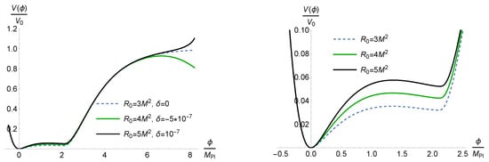
Figure 1. On the left, the inflaton potential having two plateaus for $g=2.25$ and $b=2.89$ with $V_0={\displaystyle \frac{3}{4}}{M}^2$. On the right, zoom of the potential for lower values of $\varphi$ with a near-inflection point. The potential is unstable for negative values of $\delta$ and has the infinite plateau for $\delta =0$ describing the Starobinsky inflation.

The standard SR conditions are given by ${ϵ}_{\mathrm{sr}}\ll 1$ and $\left|{\eta }_{\mathrm{sr}}\right|\ll 1$, where

$${ϵ}_{\mathrm{sr}}\left(\varphi \right)={\displaystyle \frac{1}{2}}{\left({\displaystyle \frac{V^{\prime }\left(\varphi \right)}{V\left(\varphi \right)}}\right)}^2\mathrm{and}{\eta }_{\mathrm{sr}}\left(\varphi \right)={\displaystyle \frac{V^{″}\left(\varphi \right)}{V\left(\varphi \right)}},$$

(6)

while the time clock is conveniently defined by the number N of e-folds, $N\left(t\right)={\int }_{t}H\left(\tilde{t}\right)d\tilde{t}$, where $H\left(t\right)$ is the Hubble function. The CMB tilt $n_s$ of scalar perturbations and the tensor-to-scalar ratio r are related to the values of the SR parameters at the horizon exit with the standard pivot scale $k_{\ast }=0.05{\mathrm{Mpc}}^{-1}$. In the model [8], the tensor-to-scalar ratio r is well inside the current observational bound, $r<0.032$, and the tilt $n_s$ agrees within $1\sigma$ with the current CMB measurements [4,5,6], $n_s=0.9649\pm 0.0042$, with $\delta \sim {10}^{-7}$.

The primordial spectrum $P_{\zeta }\left(k\right)$ of 3-dimensional scalar (density) perturbations $\zeta \left(x\right)$ in a flat Friedman universe is defined by the 2-point correlation function as

$$⟨{\displaystyle \frac{\delta \zeta \left(x\right)}{\zeta }}·{\displaystyle \frac{\delta \zeta \left(y\right)}{\zeta }}⟩=\int {\displaystyle \frac{d^{3}k}{k^3}}{e}^{ik·(x-y)}{\displaystyle \frac{P_{\zeta }\left(k\right)}{P_0}},$$

(7)

where $k=2\pi /\lambda$ is the co-moving number. The scale k is simply related to the e-folds number N via $N=-{\int }^{k}d\tilde{k}/\tilde{k}$. Though the USR phase has dynamics different from the SR one, the dimensionless power spectrum of scalar perturbations in the SR approximation

$$P_{\zeta }={\displaystyle \frac{H^2}{8{\pi }^2{ϵ}_{\mathrm{sr}}}}$$

(8)

appears to be a good approximation in the USR phase as well. The power spectrum is given in Figure 2 in the best case given by the 3rd row of Table 1 in Ref. [8]. Accordingly, the SR parameter ${ϵ}_{\mathrm{sr}}$ drops to very low values, indicating the USR phase.

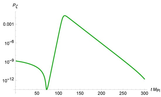
Figure 2. The primordial power spectrum $P_{\zeta }\left(t\right)$ of scalar perturbations from Equation (8). A derivation of the spectrum from the Mukhanov–Sasaki equation leads to a very similar result.

The power spectrum-related observables in our model best case are given by [8]

$$n_s\approx 0.965,r\approx 0.0095,M_{\mathrm{PBH}}\approx 1.0·{10}^{20}\mathrm{g}.$$

(9)

The corresponding peak in the power spectrum of Figure 2 can be roughly approximated by the lognormal fit [23]

$$P_{\zeta }^{\mathrm{peak}}\left(k\right)\approx {\displaystyle \frac{A_{\zeta }}{\sqrt{2\pi }\mathsf{\Delta }}}\exp \left[{\displaystyle \frac{-{\ln }^2(k/k_p)}{2{\mathsf{\Delta }}^2}}\right]$$

(10)

with the amplitude $A_{\zeta }\approx 0.06$ and the width $\mathsf{\Delta }\approx 1.5$, where $k_p\approx 4.5·{10}^{12}{\mathrm{Mpc}}^{-1}$ is the location of the peak; see Figure 3.

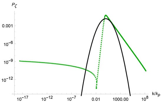
Figure 3. The primordial power spectrum $P_{\zeta }\left(k\right)$ of scalar perturbations (in green) and the lognormal fit (in black). The green lines (both dotted and solid) represent the results of our numerical calculations of the spectrum. The solid green line against the dotted green line highlights a slightly better agreement with Equation (8).

The value of ${\eta }_{\mathrm{sr}}\approx -0.025$ in the USR phase practically does not depend upon the parameters $R_0$ and $\delta$. The more illuminating functions are given by the Hubble flow parameters

$${ϵ}_H=-{\displaystyle \frac{\dot{H}}{H^2}},{\eta }_H={ϵ}_H-{\displaystyle \frac{{\dot{ϵ}}_H}{2{ϵ}_{H}H}}.$$

(11)

Though ${ϵ}_{\mathrm{sr}}$ and ${ϵ}_H$ can be identified, the evolution of ${\eta }_{\mathrm{sr}}$ and ${\eta }_H$ is different during the USR phase; see Figure 4.

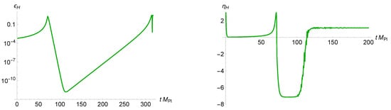
Figure 4. The evolution of ${ϵ}_H\left(t\right)$ and ${\eta }_H\left(t\right)$ with the initial conditions ${\varphi }_{in}=7.01$ and ${\dot{\varphi }}_{in}=0$, and the parameters $\delta =2.7\times {10}^{-8}$ and $R_0=3.0M^2$. In the USR phase, the value of ${\eta }_H\left(t\right)$ is close to $-6$.

3. PBH-Induced GW and PBH-DM Density Fraction

PBH production in the early universe leads to stochastic gravitational waves (GWs) different from primordial GWs caused by inflation. The current energy density fraction of those PBH-induced GWs can be computed in the second order with respect to perturbations as [24,25]

$$\begin{array}{cc}\hfill {\mathsf{\Omega }}_{\mathrm{GW}}\left(k\right)=& {\displaystyle \frac{c_g{\mathsf{\Omega }}_{r,0}}{36}}{\int }_0^{{\displaystyle \frac{1}{\sqrt{3}}}}\mathrm{d}d{\int }_{{\displaystyle \frac{1}{\sqrt{3}}}}^{\infty }\mathrm{d}s{\left[{\displaystyle \frac{(d^2-1/3)(s^2-1/3)}{s^2-d^2}}\right]}^2\times \hfill \\ \hfill & {\mathcal{P}}_{\zeta }\left({\displaystyle \frac{k\sqrt{3}}{2}}(s+d)\right){\mathcal{P}}_{\zeta }\left({\displaystyle \frac{k\sqrt{3}}{2}}(s-d)\right)\left[{\mathcal{I}}_c{(d,s)}^2+{\mathcal{I}}_s{(d,s)}^2\right],\hfill \end{array}$$

(12)

where the functions ${\mathcal{I}}_c(d,s)$ and ${\mathcal{I}}_s(d,s)$ are

$$\begin{array}{cc}\hfill {\mathcal{I}}_c(d,s)& =-36\pi {\displaystyle \frac{{(s^2+d^2-2)}^2}{{(s^2-d^2)}^3}}\theta (s-1),\hfill \\ \hfill {\mathcal{I}}_s(d,s)& =-36{\displaystyle \frac{s^2+d^2-2}{{(s^2-d^2)}^2}}\left[{\displaystyle \frac{s^2+d^2-2}{(s^2-d^2)}}\ln \left|{\displaystyle \frac{d^2-1}{s^2-1}}\right|+2\right],\hfill \end{array}$$

(13)

with ${\mathsf{\Omega }}_{r,0}\sim 8.6\times {10}^{-5}$ being the current energy density fraction of radiation, $\theta (s-1)$ is the step function, and $c_g\approx 0.4$.

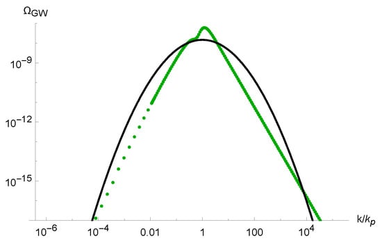
A numerical calculation of Equation (12) with the power spectrum in Figure 2 yields the result given in Figure 5 in green. The numerical plot can be well approximated by the lognormal fit given in Figure 5 in black, with the analytic formula

$${\mathrm{GW}}^{\left(k\right)}={\displaystyle \frac{A_{\mathrm{GW}}}{\sqrt{2\pi }{\sigma }_{\mathrm{GW}}}}\exp \left[-{\displaystyle \frac{{\ln }^2(k/k_p)}{2{\sigma }_{\mathrm{GW}}^2}}\right],$$

(14)

the amplitude $A_{\mathrm{GW}}\approx 5.6·{10}^{-8}$, and the width ${\sigma }_{\mathrm{GW}}\approx \mathsf{\Delta }/\sqrt{2}\approx 1.06$, where $\mathsf{\Delta }$ is the width of the power spectrum in Figure 2. The ${\mathsf{\Omega }}_{\mathrm{GW}}^{\mathrm{peak}}\left(k\right)$ near the peak is roughly given by ${10}^{-6}{\mathcal{P}}_{\zeta }^2\left(k\right)$, in agreement with the estimates in Refs. [26,27].

Figure 5. The PBH-induced stochastic GW density fraction (in green) with the lognormal fit (in black) in Equation (14). The dotted and solid green lines mean that the log-normal fit (14) applies only to the top of the peak.

The induced GW frequencies $f_p$ are related to the PBH masses as [28]

$$f_p\approx 5.7{\left({\displaystyle \frac{M_{\odot }}{M_{\mathrm{PBH}}}}\right)}^{1/2}{10}^{-9}\mathrm{Hz},$$

(15)

where the Sun mass is given by $M_{\odot }\approx 2·{10}^{33}$ g. Given the PBH masses of ${10}^{20}$ g, as in our model, it results in the GW frequency $f_p\approx 0.0255$ Hz. It is higher than the GW frequencies between 3 and 400 nHz detected by NANOGrav [29]. A detection of the GW peak with that frequency in the ${10}^{-2}$ Hz range would provide observational support to our model provided the peak is due to generation of the secondary GWs. A more specific comparison of our predictions with future GW observations is possible by plotting the GW spectrum in our model against the expected sensitivity curves in future space-based gravitational interferometers such as LISA [30,31], TianQin [32], Taiji [33,34], and DECIGO [35]; see Figure 6, where we have used Refs. [36,37,38] for the colored curves. The space-based experiments are expected to be sensitive to stochastic GWs in the frequencies between ${10}^{-3}$ and ${10}^{-1}$ Hz, while the predicted black curve in Figure 6 in our model belongs to that frequency range.

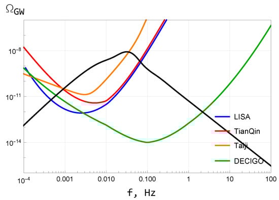
Figure 6. The GW density induced by the power spectrum of scalar perturbations in our model (in black) against the expected sensitivity curves for future space-based GW experiments (in color).

The PBH-in-DM density fraction $f\left(k\right)$ on scale k can be estimated in the Press–Schechter formalism [39] as

$$f\left(k\right)={\displaystyle \frac{{\mathsf{\Omega }}_{\mathrm{PBH}}\left(k\right)}{{\mathsf{\Omega }}_{\mathrm{DM}}}}\approx {\displaystyle \frac{1.2·{10}^{24}{\beta }_f\left(k\right)}{\sqrt{M_{\mathrm{PBH}}\left(k\right){\mathrm{g}}^{-1}}}}\approx 17.1(k·\mathrm{Mpc}){\beta }_f\left(k\right),$$

(16)

where [40,41]

$${\beta }_f\left(k\right)\simeq {\displaystyle \frac{\sigma \left(k\right)}{\sqrt{2\pi }{\delta }_c}}{e}^{-{\displaystyle \frac{{\delta }_c^2}{2{\sigma }^2\left(k\right)}}},{\sigma }^2\left(k\right)={\displaystyle \frac{16}{81}}\int {\displaystyle \frac{dq}{q}}{\left({\displaystyle \frac{q}{k}}\right)}^4{e}^{-q^2/k^2}{P}_{\zeta }\left(q\right),$$

(17)

with the constant ${\delta }_c$ depending upon the shape of the PBH peak in the power spectrum and representing the density threshold for PBH formation. The integral in Equation (17) can be estimated as

$${\sigma }^2\approx {\displaystyle \frac{3.84}{81}}{P}_{\zeta }^{\mathrm{peak}},$$

(18)

where $P_{\zeta }^{\mathrm{peak}}$ is the value of the power spectrum at the PBH peak. Then, Equations (16) and (17) imply

$$f\left(k\right)\sim {\displaystyle \frac{{10}^{23}}{\sqrt{M_{\mathrm{PBH}}\left(k\right){\mathrm{g}}^{-1}}}}\left({\displaystyle \frac{\sqrt{P_{\zeta }^{\mathrm{peak}}}}{{\delta }_c}}\right)e^{-9.3{\delta }_c^2/P_{\zeta }^{\mathrm{peak}}}.$$

(19)

This equation demonstrates the high sensitivity of the PBH-in-DM fraction upon the value of ${\delta }_c^2/P_{\zeta }^{\mathrm{peak}}$. In the case of the power spectrum in Figure 2, we have ${\delta }_c\approx 0.45$ and $P_{\zeta }^{\mathrm{peak}}\approx 0.05$. Given the range of the model parameters in Ref. [8], Equation (19) gives the PBH fraction in DM between $0.1\%$ and $100\%$. In addition, the Press–Schechter formalism itself should be considered with a grain of salt because it was found to be unreliable [42,43,44]. It is also worth mentioning that even a small PBH fraction could have an important role in cosmology [21].

4. Loop Corrections

In the $\delta N$ formalism [19] for single-field inflation, a scalar (comoving curvature) perturbation $\delta N\equiv \zeta$ is a function of variation $\delta \varphi$ of inflaton ${\varphi }_i$ at its initial value,

$$\delta N=N^{\prime }\left(\varphi \right)\delta \varphi +{\displaystyle \frac{N^{″}\left(\varphi \right)}{2!}}\delta {\varphi }^2+{\displaystyle \frac{N^{‴}\left(\varphi \right)}{3!}}\delta {\varphi }^3+\dots ,$$

(20)

where perturbations are not assumed to be small. The power spectrum of scalar perturbations is defined by a two-point function of Fourier components ${\zeta }_{\mathbf{p}}$ as

$$⟨{\zeta }_{{\mathbf{p}}_{\mathbf{1}}}{\zeta }_{{\mathbf{p}}_{\mathbf{2}}}⟩={\left(2\pi \right)}^3{\delta }^3({\mathbf{p}}_{\mathbf{1}}+{\mathbf{p}}_{\mathbf{2}})P\left(p\right),P_{\zeta }\left(p\right)={\displaystyle \frac{k^3}{2{\pi }^2}}P\left(p\right),$$

(21)

where

$${\zeta }_{\mathbf{p}}=N^{\prime }\delta {\varphi }_{\mathbf{p}}+{\displaystyle \frac{N^{″}}{2!}}\int {\displaystyle \frac{d^{3}q}{{\left(2\pi \right)}^3}}\delta {\varphi }_{\mathbf{q}}\delta {\varphi }_{\mathbf{p}-\mathbf{q}}+{\displaystyle \frac{N^{‴}}{3!}}\int {\displaystyle \frac{d^3{q}_1}{{\left(2\pi \right)}^3}}{\displaystyle \frac{d^3{q}_2}{{\left(2\pi \right)}^3}}\delta {\varphi }_{{\mathbf{q}}_{\mathbf{1}}}\delta {\varphi }_{{\mathbf{q}}_{\mathbf{2}}}\delta {\varphi }_{\mathbf{p}-{\mathbf{q}}_{\mathbf{1}}-{\mathbf{q}}_{\mathbf{2}}}+\dots$$

(22)

in terms of external 3D momenta $\mathbf{p}$ and loop momenta $\mathbf{q}$. Substituting Equation (22) into Equation (21) yields the loop expansion of the power spectrum $P_{\zeta }\left(p\right)$. In order to apply that to a particular model, one has to know the function $N\left(\varphi \right)$ explicitly. It was derived in Ref. [16],

$$N_{\mathrm{total}}\left({\varphi }_i\right)\simeq {\displaystyle \frac{1}{{\eta }_{\mathrm{sr}}}}\ln \left[1+{\displaystyle \frac{{\eta }_{\mathrm{sr}}}{\sqrt{2{ϵ}_{\mathrm{sr}}}}}({\varphi }_i-{\varphi }_s)\right]-{\displaystyle \frac{1}{3}}\ln \left[1+{\displaystyle \frac{3({\varphi }_s-{\varphi }_e)}{{\pi }_s}}\right]+{\displaystyle \frac{1}{{\eta }_{\mathrm{V}}}}\ln [-2{\eta }_{\mathrm{V}}{\pi }_e-6\sqrt{2{ϵ}_{\mathrm{V}}}],$$

(23)

where the first term refers to the SR(I) phase with the initial value ${\varphi }_i$ and the end value ${\varphi }_s$, the second term refers to the USR phase with the initial momentum value ${\pi }_s$ and the end momentum value ${\pi }_e$, and the third terms refers to the SR(II) phase with the slow-roll parameters ${ϵ}_{\mathrm{V}}$ and ${\eta }_{\mathrm{V}}$. The subscripts $(s,e)$ refer to values of any quantity at the start and end of the USR phase, respectively. The leading contribution comes from the first term in Equation (23).

To compute loop corrections, one has to calculate the derivatives $N^{\left(n\right)}\left(\varphi \right)$. The first three derivatives can be estimated as follows:

$$N^{\prime }\approx {\displaystyle \frac{1}{\sqrt{2{ϵ}_s}}}\approx {\displaystyle \frac{e^{-3\mathsf{\Delta }{N}_{\mathrm{USR}}}}{\sqrt{2{ϵ}_e}}},N^{″}\approx -{\displaystyle \frac{{\eta }_{\mathrm{sr}}}{2{ϵ}_s}},N^{‴}\approx {\displaystyle \frac{2{\eta }_{\mathrm{sr}}^2}{{\left(2{ϵ}_s\right)}^{3/2}}},$$

(24)

where $\mathsf{\Delta }{N}_{\mathrm{USR}}$ is the duration of the USR phase and ${\eta }_{\mathrm{sr}}\equiv {\eta }_{\mathrm{sr}}\left({\varphi }_s\right)$.

To compute loop corrections to the amplitude of the power spectrum, we considered the effective action up to the third order with respect to $\delta \varphi (\mathbf{x},t)$ on the background $\varphi \left(t\right)$,

$$S_{\delta \varphi }=S_{\delta \varphi }^{\left(2\right)}+S_{\delta \varphi }^{\left(3\right)}={\displaystyle \frac{1}{2}}\int d^{4}x\sqrt{-g}\left(g_{\mu \nu }{\partial }^{\mu }\delta \varphi {\partial }^{\nu }\delta \varphi -V_{,\varphi \varphi }\delta {\varphi }^2\right)+{\displaystyle \frac{1}{2}}\int d^{4}x\sqrt{-g}\left(-{\displaystyle \frac{1}{3}}{V}_{,\varphi \varphi \varphi }\delta {\varphi }^3\right).$$

(25)

A comparable contribution of the quartic coupling $V_{,\varphi \varphi \varphi \varphi }$ was investigated in Ref. [45]. When using the FLRW background, the effective action reads

$$S_{\delta \varphi }={\displaystyle \frac{1}{2}}\int d^{4}x{a}^3\left(t\right)\left[{\dot{\delta \varphi }}^2-a^{-2}\left(t\right){(\partial \delta \varphi )}^2-V_{,\varphi \varphi }\delta {\varphi }^2\right]+\int d^{4}x\left[-{\displaystyle \frac{a^3\left(t\right)}{3!}}{V}_{,\varphi \varphi \varphi }\delta {\varphi }^3\right],$$

(26)

where $\partial \equiv {\sum }_i{\partial }_i$ is a sum of spatial derivatives. The mode functions arising in the solutions to classical equations of motion from the action (26) with Bunch–Davies initial conditions,

$$u_k\left(\tau \right)={\displaystyle \frac{H}{\sqrt{2k^3}}}(1+ik\tau )e^{-ik\tau },$$

(27)

are written down in terms of the conformal time $d\tau ={\displaystyle \frac{dt}{a}}$, where $-\infty <\tau \le 0$. The CMB modes that left the horizon during inflation are given by $u_k\left(0\right)={\displaystyle \frac{H}{\sqrt{2k^3}}}$.

Canonical quantization implies a decomposition into positive and negative parts, as well as the commutation relations (in the interaction picture)

$$\begin{array}{cc}\hfill & \delta {\varphi }_{\mathbf{k}}^I\left(\tau \right)=\delta {\varphi }_{\mathbf{k}}^{+}\left(\tau \right)+\delta {\varphi }_{\mathbf{k}}^{-}\left(\tau \right)=u_k\left(\tau \right)a_{\mathbf{k}}+u_k^{\ast }\left(\tau \right)a_{-\mathbf{k}}^{†},\hfill \\ \hfill & [a_{\mathbf{p}},a_{\mathbf{q}}^{†}]={\left(2\pi \right)}^3{\delta }^3(\mathbf{p}-\mathbf{q}),[a_{\mathbf{p}},a_{\mathbf{q}}]=[a_{\mathbf{p}}^{†},a_{\mathbf{q}}^{†}]=0.\hfill \end{array}$$

(28)

To obtain the one-loop correction according to Equations (21) and (22), one has to evaluate the three-point correlation function. For this purpose, we applied the in-in formalism that gives

$$⟨\delta {\varphi }_{\mathbf{p}}\delta {\varphi }_{\mathbf{q}}\delta {\varphi }_{-\mathbf{p}-\mathbf{q}}⟩=⟨\overline{T}{e}^{i{\int }_{t_0}^{t}d\tilde{t}{H}_{\mathrm{int}}}\delta {\varphi }_{\mathbf{p}}^I\delta {\varphi }_{\mathbf{q}}^I\delta {\varphi }_{-\mathbf{p}-\mathbf{q}}^{I}T{e}^{-i{\int }_{t_0}^{t}d\tilde{t}{H}_{\mathrm{int}}}⟩,$$

(29)

where T and $\overline{T}$ stand for the time ordering and anti-time ordering, respectively, $t_0$ and t are the times associated with the subhorizon and superhorizon scales, respectively, and $H_{\mathrm{int}}\left(\tilde{t}\right)$ is the interaction Hamiltonian in the third order,

$$H_{\mathrm{int}}\left(\tilde{t}\right)={\displaystyle \frac{1}{3!}}{a}^3\left(\tilde{t}\right)V_{,\varphi \varphi \varphi }\int d^{3}x{\left(\delta {\varphi }^I(\mathbf{x},\tilde{t})\right)}^3={\displaystyle \frac{1}{3!{\left(2\pi \right)}^6}}{a}^3\left(\tilde{t}\right)V_{,\varphi \varphi \varphi }\int d^{3}k{d}^3\lambda \delta {\varphi }_{\mathbf{k}}^I\left(\tilde{t}\right)\delta {\varphi }_{\mathsf{\lambda }}^I\left(\tilde{t}\right)\delta {\varphi }_{-\mathbf{k}-\mathsf{\lambda }}^I\left(\tilde{t}\right).$$

(30)

The standard (Friedmann and Klein–Gordon) equations of motion yield the following asymptotic approximation for the third derivative of the potential in terms of the Hubble flow parameters (11):

$$V_{,\varphi \varphi \varphi }\simeq -{\displaystyle \frac{3H\dot{{\eta }_H}}{2\sqrt{2{ϵ}_H}}}.$$

(31)

Expanding the T-exponentials in Equation (29) to the first order with respect to $H_{\mathrm{int}}$, we find

$$\begin{array}{cc}\hfill & ⟨\delta {\varphi }_{\mathbf{p}}\left(t\right)\delta {\varphi }_{\mathbf{q}}\left(t\right)\delta {\varphi }_{-\mathbf{p}-\mathbf{q}}\left(t\right)⟩\approx -i{\int }_{t_0}^{t}d\tilde{t}⟨[\delta {\varphi }_{\mathbf{p}}^I\left(t\right)\delta {\varphi }_{\mathbf{q}}^I\left(t\right)\delta {\varphi }_{-\mathbf{p}-\mathbf{q}}^I\left(t\right),H^{int}\left(\tilde{t}\right)]⟩\hfill \\ \hfill & =2\mathrm{Im}\left({\int }_{t_0}^{t}d\tilde{t}⟨\delta {\varphi }_{\mathbf{p}}^I\left(t\right)\delta {\varphi }_{\mathbf{q}}^I\left(t\right)\delta {\varphi }_{-\mathbf{p}-\mathbf{q}}^I\left(t\right)H^{int}\left(\tilde{t}\right)⟩\right).\hfill \end{array}$$

(32)

After substituting Equations (27), (28), (30), and (31) into Equation (32) and using Wick’s theorem, we derived the three-point correlator as follows:

$$\begin{array}{cc}\hfill & ⟨\delta {\varphi }_{\mathbf{p}}\delta {\varphi }_{\mathbf{q}}\delta {\varphi }_{-\mathbf{p}-\mathbf{q}}⟩=\hfill \\ \hfill & =-{\displaystyle \frac{1}{2{\left(2\pi \right)}^6}}\mathrm{Im}\left({\int }_{-\infty }^{0}d\tilde{\tau }{a}^3\left(\tilde{\tau }\right){\displaystyle \frac{H{\eta }^{\prime }\left(\tilde{\tau }\right)}{\sqrt{2ϵ}}}\int d^{3}k{d}^3\lambda ⟨\delta {\varphi }_{\mathbf{p}}^{+}\delta {\varphi }_{\mathbf{q}}^{+}\delta {\varphi }_{-\mathbf{p}-\mathbf{q}}^{+}\delta {\varphi }_{\mathbf{k}}^{-}\left(\tilde{\tau }\right)\delta {\varphi }_{\mathsf{\lambda }}^{-}\left(\tilde{\tau }\right)\delta {\varphi }_{-\mathbf{k}-\mathsf{\lambda }}^{-}\left(\tilde{\tau }\right)⟩\right)\hfill \\ \hfill & =-{\displaystyle \frac{\mathsf{\Delta }\eta }{2{\left(2\pi \right)}^6}}\mathrm{Im}\left({\displaystyle \frac{H_e{a}_e^3}{\sqrt{2{ϵ}_e}}}\int d^{3}k{d}^3\lambda ⟨\delta {\varphi }_{\mathbf{p}}^{+}\left(\tau \right)\delta {\varphi }_{\mathbf{q}}^{+}\left(\tau \right)\delta {\varphi }_{-\mathbf{p}-\mathbf{q}}^{+}\left(\tau \right)\delta {\varphi }_{\mathbf{k}}^{-}\left({\tau }_e\right)\delta {\varphi }_{\mathsf{\lambda }}^{-}\left({\tau }_e\right)\delta {\varphi }_{-\mathbf{k}-\mathsf{\lambda }}^{-}\left({\tau }_e\right)⟩\right)\hfill \\ \hfill & \approx {\displaystyle \frac{3!{\left(2\pi \right)}^3\left|\mathsf{\Delta }\eta \right|}{2}}\mathrm{Im}\left({\displaystyle \frac{H_e^4{a}_e^3}{\sqrt{2{ϵ}_e}}}{\displaystyle \frac{H_0^3{(1-iq{\tau }_e)}^2}{{\left(2q^3\right)}^{2}2p^3}}{e}^{2iq{\tau }_e}\right),\hfill \end{array}$$

(33)

where the $H\left(0\right)=H_0$ denotes the Hubble value during the SR(I), and the reference time was chosen at $\tau =0$ because we were only interested in the power spectrum on superhorizon scales relevant to CMB, and $p\ll q$. To avoid divergences, the vacuum expectation value was normalized by the volume of the entire system.

The dynamics of the parameter ${\eta }_H$ implies it is essentially constant everywhere except for the moments of a decrease or an increase (corresponding to ${\tau }_s$ and ${\tau }_e$, respectively), while the moment of the increase is particularly significant (see Figure 4). The approximate solution (23) to the equations of motion in our model is smooth as well as the corresponding ${\eta }_H\left(t\right)$ function defined by the second Equation (11). To simplify our calculations, we employed the derivative of ${\eta }_H$ with respect to the conformal time as the (Dirac) delta function, ${\eta }_H^{\prime }\left(\tau \right)\sim \delta (\tau -{\tau }_e)\mathsf{\Delta }\eta$, where $\mathsf{\Delta }\eta \approx -6$ is the depth of the pit, inside integrations, which corresponds to a sharp transition. Via integration, the delta function fixes the entire integrand at the time ${\tau }_e$ corresponding to the end of the USR stage.

Equations (20)–(22) lead to a recovery of the tree-level contribution (8) as the leading term in the loop expansion of the power spectrum, as well as the first (one-loop) contribution as follows:

$$P_{\zeta }^{1-\mathrm{loop}}\left(p\right)\equiv {\displaystyle \frac{N^{\prime }{N}^{″}}{2}}\int {\displaystyle \frac{d^{3}q}{{\left(2\pi \right)}^3}}⟨\delta {\varphi }_{\mathbf{p}}\delta {\varphi }_{\mathbf{q}}\delta {\varphi }_{-\mathbf{p}-\mathbf{q}}⟩.$$

(34)

After substituting Equations (24) and (33) into Equation (34), we found

$$\begin{array}{cc}\hfill & P_{\zeta }^{1-\mathrm{loop}}\left(p\right)\approx {\displaystyle \frac{{\eta }_{\mathrm{sr}}{e}^{-3\mathsf{\Delta }{N}_{\mathrm{USR}}}}{2\sqrt{2{ϵ}_e}2{ϵ}_s}}{\int }_{\mathrm{USR}}dq\left(4\pi q^2\right){\displaystyle \frac{3!\left|\mathsf{\Delta }\eta \right|}{2}}\mathrm{Im}\left({\displaystyle \frac{H_e^4{a}_e^3}{\sqrt{2{ϵ}_e}}}{\displaystyle \frac{H_0^3{(1-iq{\tau }_e)}^2}{{\left(2q^3\right)}^{2}2p^3}}{e}^{2iq{\tau }_e}\right)\hfill \\ \hfill & \approx {\eta }_{\mathrm{sr}}{e}^{-3\mathsf{\Delta }{N}_{\mathrm{USR}}}{P}_{\zeta }\left(p\right)P_{\zeta }^{\mathrm{PBH}}{\displaystyle \frac{{\left(2\pi \right)}^3\left|\mathsf{\Delta }\eta \right|}{4}}\left({\displaystyle \frac{H_0}{H_e}}\right),\hfill \end{array}$$

(35)

where $P_{\zeta }^{\mathrm{PBH}}\sim {10}^{-2}$ is the fixed amplitude of the power spectrum on the small scales associated with the short-wavelength PBH modes exiting the horizon during the USR phase of inflation. The value of $H_0/H_e\approx 5$ defines the ratio of the inflation and PBH scales in our model.

It is evident from Equation (35) that the dependence of the one-loop correction upon the slow-roll parameter ${\eta }_{sr}$ comes from the second derivative $N^{″}$, the exponential factor depending upon $\mathsf{\Delta }{N}_{\mathrm{USR}}$ arises from the first derivative $N^{\prime }$, and the dependence upon $P_{\zeta }^{\mathrm{PBH}}$ and $\mathsf{\Delta }\eta$ comes from the third derivative $V_{,\varphi \varphi \varphi }$, namely, from ${\eta }^{\prime }\left(\tau \right)$.

A detailed calculation of the higher-loop corrections is highly involved and is not given here. However, it is possible to obtain a rough estimate of the two-loop correction by using the approximative formula given in Ref. [16],

$$P_{\zeta }^{2-\mathrm{loop}}\left(p\right)\approx {\displaystyle \frac{N^{\prime }{N}^{‴}}{3!}}|\delta {\varphi }_{\mathbf{p}}{|}^2\int {\displaystyle \frac{d^{3}q}{{\left(2\pi \right)}^3}}{\left|\delta {\varphi }_{\mathbf{q}}\right|}^2\sim {\eta }_{\mathrm{sr}}^2\mathsf{\Delta }{N}_{\mathrm{USR}}{P}_{\zeta }\left(p\right)P_{\zeta }^{\mathrm{PBH}}.$$

(36)

In our model, according to the plot on the right-hand side of Figure 4, we have $\mathsf{\Delta }{N}_{\mathrm{USR}}\approx 3.1$.

Therefore, the relative size of the one-loop and two-loop corrections from PBH production to the power spectrum at the CMB pivot scale $k^{\ast }=0.05$ are

$${\displaystyle \frac{P_{\zeta }^{1-\mathrm{loop}}(k^{\ast }=0.05)}{P_{\zeta }(k^{\ast }=0.05)}}\approx {\eta }_{\mathrm{sr}}{e}^{-3\mathsf{\Delta }{N}_{\mathrm{USR}}}{P}_{\zeta }^{\mathrm{PBH}}{\displaystyle \frac{{\left(2\pi \right)}^3\left|\mathsf{\Delta }\eta \right|}{4}}\left({\displaystyle \frac{H_0}{H_e}}\right)\approx {10}^{-3}$$

(37)

and

$${\displaystyle \frac{P_{\zeta }^{2-\mathrm{loop}}(k^{\ast }=0.05)}{P_{\zeta }(k^{\ast }=0.05)}}\sim {\eta }_{\mathrm{sr}}^2\mathsf{\Delta }{N}_{\mathrm{USR}}{P}_{\zeta }^{\mathrm{PBH}}\approx {10}^{-5},$$

(38)

where we used $P_{\zeta }(k^{\ast }=0.05)\approx 2·{10}^{-9}$ for the CMB power spectrum. Therefore, the one-loop contribution is suppressed by the factor ${\eta }_{\mathrm{sr}}{e}^{-3\mathsf{\Delta }{N}_{\mathrm{USR}}}$, whereas the two-loop contribution is suppressed by ${\eta }_{\mathrm{sr}}^2\mathsf{\Delta }{N}_{\mathrm{USR}}$ (we recall that ${\eta }_{\mathrm{sr}}\approx -0.025$ in our model). As regards the higher n-loop corrections, their structure includes the suppression factor ${\eta }_{\mathrm{sr}}^n{P}_{\zeta }^{\mathrm{PBH}}\sim {10}^{-2n-2}$ so that they are expected to be negligible too.

The relative smallness of loop corrections in our model is in agreement with the considerations of Refs. [16,17,46,47,48] but in disagreement with the results of Refs. [13,14]. Our calculations were based on the $\delta N$ formalism, also used in Ref. [16], whereas the calculations performed in Refs. [13,14] were based on the in-in formalism. It is beyond the scope of our investigation to compare the two formalisms. 2

The amplitude of the power spectrum during USR was fixed in our approach, while we effectively assumed a sharp transition in part of our analytic calculations. The sharpness of transitions can be quantitatively estimated by the parameter h defined by [18]

$$h=6{\displaystyle \frac{\sqrt{2{ϵ}_{\mathrm{V}}}}{\stackrel{•}{\varphi }\left(t_e\right)}}=-6{\displaystyle \frac{\sqrt{2{ϵ}_{\mathrm{V}}}}{{\pi }_e}}=-6\sqrt{{\displaystyle \frac{{ϵ}_{\mathrm{V}}}{{ϵ}_s}}}{e}^{3\mathsf{\Delta }{N}_{\mathrm{USR}}},$$

(39)

where ${\pi }_e$ is the inflaton momentum at the end of the USR inflation, ${ϵ}_s\approx 1$ is the SR parameter at the end of the SR(I) or at the beginning of USR, and ${ϵ}_{\mathrm{V}}$ is the SR parameter at the end of USR. In our model, by using Figure 4, we obtained $h\approx -0.66$, which implies a sharp (though rather mild) transition because, on the one hand, $\left|h\right|$ is not much less than one but on the other hand, it is still away from a truly sharp transition with the “standard” value $h=-6$ used in Ref. [13]. As was demonstrated in Ref. [45], the lower value of h also justifies ignoring the quartic coupling in our analysis. As a result, the one-loop correction in our model appeared to be small against the tree-level contribution, as in Refs. [17,49].

5. Conclusions

The main new results of this paper were given by Figure 6, Equations (19) and (35). It follows that the modified gravity model [8] of Starobinsky inflation with PBH production may generate a significant part (or the whole) of dark matter from PBHs, while it was not ruled out by quantum loop corrections because the latter were relatively small by a factor of ${10}^{-3}$ against the tree-level (classical) contribution. The key role in the last conclusion was played by the derivatives of the function $N\left(\varphi \right)$ during the USR phase, describing superhorizon curvature perturbations in the $\delta N$ formalism, which led to the suppression of loop contributions. It is worth mentioning that our results only apply to the particular phenomenological model of PBH production related to Starobinsky inflation.

The predicted frequency $f_p\approx 2.55·{10}^{-2}$ Hz of the PBH production-induced stochastic GWs is in the range between ${10}^{-3}$ Hz and ${10}^{-1}$ Hz of the frequencies that are expected to be sensitive to the future space-based gravitational interferometers.

As was recently pointed out in the literature [50,51,52,53], the standard result for the primordial black hole survival at present, based on the Hawking semiclassical evaporation formula, may be relaxed below ${10}^{15}$ g, when going beyond the semiclassical approximation. Should this be the case, fine-tuning the parameters in our model for efficient PBH production (needed for DM) may be significantly relaxed.

References

- Starobinsky, A.A. A new type of isotropic cosmological models without singularity. Phys. Lett. B 1980, 91, 99–102. [Google Scholar] [CrossRef]
- Ketov, S.V. On the equivalence of Starobinsky and Higgs inflationary models in gravity and supergravity. J. Phys. A 2020, 53, 084001. [Google Scholar] [CrossRef]
- Ivanov, V.R.; Ketov, S.V.; Pozdeeva, E.O.; Vernov, S.Y. Analytic extensions of Starobinsky model of inflation. J. Cosmol. Astropart. Phys. 2022, 3, 058. [Google Scholar] [CrossRef]
- Akrami, Y.; Arroja, F.; Ashdown, M.; Aumont, J.; Baccigalupi, C.; Ballardini, M.; Banday, A.J.; Barreiro, R.B.; Bartolo, N.; Basak, S.; et al. Planck 2018 results. X. Constraints on inflation. Astron. Astrophys. 2020, 641, A10. [Google Scholar] [CrossRef]
- Ade, P.A. et al. [BICEP, Keck Collaboration] Improved Constraints on Primordial Gravitational Waves using Planck, WMAP, and BICEP/Keck Observations through the 2018 Observing Season. Phys. Rev. Lett. 2021, 127, 151301. [Google Scholar] [CrossRef]
- Tristram, M.; Banday, A.J.; Górski, K.M.; Keskitalo, R.; Lawrence, C.R.; Andersen, K.J.; Barreiro, R.B.; Borrill, J.; Colombo, L.P.L.; Eriksen, H.K.; et al. Improved limits on the tensor-to-scalar ratio using BICEP and Planck data. Phys. Rev. D 2022, 105, 083524. [Google Scholar] [CrossRef]
- Frolovsky, D.; Ketov, S.V.; Saburov, S. Formation of primordial black holes after Starobinsky inflation. Mod. Phys. Lett. A 2022, 37, 2250135. [Google Scholar] [CrossRef]
- Saburov, S.; Ketov, S.V. Improved Model of Primordial Black Hole Formation after Starobinsky Inflation. Universe 2023, 9, 323. [Google Scholar] [CrossRef]
- Kamenshchik, A.Y.; Pozdeeva, E.O.; Tribolet, A.; Tronconi, A.; Venturi, G.; Vernov, S.Y. The Superpotential Method and the Amplification of Inflationary Perturbations. arXiv 2024. [Google Scholar] [CrossRef]
- Geller, S.R.; Qin, W.; McDonough, E.; Kaiser, D.I. Primordial black holes from multifield inflation with nonminimal couplings. Phys. Rev. D 2022, 106, 063535. [Google Scholar] [CrossRef]
- Cole, P.S.; Gow, A.D.; Byrnes, C.T.; Patil, S.P. Primordial black holes from single-field inflation: A fine-tuning audit. arXiv 2023. [Google Scholar] [CrossRef]
- Karam, A.; Koivunen, N.; Tomberg, E.; Vaskonen, V.; Veermäe, H. Anatomy of single-field inflationary models for primordial black holes. J. Cosmol. Astropart. Phys. 2023, 3, 013. [Google Scholar] [CrossRef]
- Kristiano, J.; Yokoyama, J. Ruling Out Primordial Black Hole Formation From Single-Field Inflation. arXiv 2024. [Google Scholar] [CrossRef]
- Choudhury, S.; Panda, S.; Sami, M. Quantum loop effects on the power spectrum and constraints on primordial black holes. J. Cosmol. Astropart. Phys. 2023, 11, 066. [Google Scholar] [CrossRef]
- Cheng, S.-L.; Lee, D.-S.; Ng, K.-W. Primordial perturbations from ultra-slow-roll single-field inflation with quantum loop effects. arXiv 2024. [Google Scholar] [CrossRef]
- Firouzjahi, H.; Riotto, A. Primordial Black Holes and Loops in Single-Field Inflation. arXiv 2023. [Google Scholar] [CrossRef]
- Davies, M.W.; Iacconi, L.; Mulryne, D.J. Numerical 1-loop correction from a potential yielding ultra-slow-roll dynamics. arXiv 2024. [Google Scholar] [CrossRef]
- Cai, Y.-F.; Chen, X.; Namjoo, M.H.; Sasaki, M.; Wang, D.-G.; Wang, Z. Revisiting non-Gaussianity from non-attractor inflation models. J. Cosmol. Astropart. Phys. 2018, 5, 12. [Google Scholar] [CrossRef]
- Abolhasani, A.A.; Firouzjahi, H.; Naruko, A.; Sasaki, M. Delta N Formalism in Cosmological Perturbation Theory; WSP: London, UK, 2019. [Google Scholar] [CrossRef]
- Appleby, S.A.; Battye, R.A.; Starobinsky, A.A. Curing singularities in cosmological evolution of F(R) gravity. J. Cosmol. Astropart. Phys. 2010, 6, 5. [Google Scholar] [CrossRef]
- Carr, B.; Kohri, K.; Sendouda, Y.; Yokoyama, J. Constraints on primordial black holes. Rept. Prog. Phys. 2021, 84, 116902. [Google Scholar] [CrossRef]
- Maeda, K.-I. Towards the Einstein-Hilbert Action via Conformal Transformation. Phys. Rev. D 2021, 39, 3159. [Google Scholar] [CrossRef]
- Frolovsky, D.; Ketov, S.V. Fitting power spectrum of scalar perturbations for primordial black hole production during inflation. Astronomy 2023, 2, 47–57. [Google Scholar] [CrossRef]
- Espinosa, J.R.; Racco, D.; Riotto, A. A Cosmological Signature of the SM Higgs Instability: Gravitational Waves. J. Cosmol. Astropart. Phys. 2018, 9, 012. [Google Scholar] [CrossRef]
- Kohri, K.; Terada, T. Semianalytic calculation of gravitational wave spectrum nonlinearly induced from primordial curvature perturbations. Phys. Rev. D 2018, 97, 123532. [Google Scholar] [CrossRef]
- Pi, S.; Sasaki, M. Gravitational Waves Induced by Scalar Perturbations with a Lognormal Peak. J. Cosmol. Astropart. Phys. 2020, 9, 037. [Google Scholar] [CrossRef]
- Domènech, G. Scalar Induced Gravitational Waves Review. Universe 2021, 7, 398. [Google Scholar] [CrossRef]
- Luca, V.D.; Franciolini, G.; Riotto, A. NANOGrav Data Hints at Primordial Black Holes as Dark Matter. Phys. Rev. Lett. 2021, 126, 041303. [Google Scholar] [CrossRef] [PubMed]
- Agazie, G. et al. [NANOGrav Collaboration] The NANOGrav 15 yr Data Set: Evidence for a Gravitational-wave Background. Astrophys. J. Lett. 2023, 951, L8. [Google Scholar] [CrossRef]
- Amaro-Seoane, P. et al. [LISA Collaboration] Laser Interferometer Space Antenna. arXiv 2017. [Google Scholar] [CrossRef]
- Smith, T.L.; Caldwell, R. LISA for Cosmologists: Calculating the Signal-to-Noise Ratio for Stochastic and Deterministic Sources. Phys. Rev. D 2019, 100, 104055. [Google Scholar] [CrossRef]
- Luo, J. et al. [TianQin Collaboration] TianQin: A space-borne gravitational wave detector. Class. Quant. Grav. 2016, 33, 035010. [Google Scholar] [CrossRef]
- Gong, X.; Lau, Y.K.; Xu, S.; Amaro-Seoane, P.; Bai, S.; Bian, X.; Cao, Z.; Chen, G.; Chen, X.; Ding, Y.; et al. Descope of the ALIA mission. J. Phys. Conf. Ser. 2015, 610, 012011. [Google Scholar] [CrossRef]
- Ruan, W.-H.; Guo, Z.-K.; Cai, R.-G.; Zhang, Y.-Z. Taiji program: Gravitational-wave sources. Int. J. Mod. Phys. A 2020, 35, 2050075. [Google Scholar] [CrossRef]
- Kudoh, H.; Taruya, A.; Hiramatsu, T.; Himemoto, Y. Detecting a gravitational-wave background with next-generation space interferometers. Phys. Rev. D 2006, 73, 064006. [Google Scholar] [CrossRef]
- Thrane, E.; Romano, J.D. Sensitivity curves for searches for gravitational-wave backgrounds. Phys. Rev. D 2013, 88, 124032. [Google Scholar] [CrossRef]
- Schmitz, K. New Sensitivity Curves for Gravitational-Wave Signals from Cosmological Phase Transitions. J. High Energy Phys. 2021, 1, 97. [Google Scholar] [CrossRef]
- Aldabergenov, Y.; Addazi, A.; Ketov, S.V. Testing Primordial Black Holes as Dark Matter in Supergravity from Gravitational Waves. Phys. Lett. B 2021, 814, 136069. [Google Scholar] [CrossRef]
- Press, W.H.; Schechter, P. Formation of galaxies and clusters of galaxies by selfsimilar gravitational condensation. Astrophys. J. 1974, 187, 425–438. [Google Scholar] [CrossRef]
- Inomata, K.; Kawasaki, M.; Mukaida, K.; Tada, Y.; Yanagida, T.T. Inflationary Primordial Black Holes as All Dark Matter. Phys. Rev. D 2017, 96, 043504. [Google Scholar] [CrossRef]
- Aldabergenov, Y.; Addazi, A.; Ketov, S.V. Primordial black holes from modified supergravity. Eur. Phys. J. C 2020, 80, 917. [Google Scholar] [CrossRef]
- Franciolini, G.; Kehagias, A.; Matarrese, S.; Riotto, A. Primordial Black Holes from Inflation and non-Gaussianity. J. Cosmol. Astropart. Phys. 2018, 3, 16. [Google Scholar] [CrossRef]
- Germani, C.; Sheth, R.K. The Statistics of Primordial Black Holes in a Radiation-Dominated Universe: Recent and New Results. Universe 2023, 9, 421. [Google Scholar] [CrossRef]
- Figueroa, D.G.; Raatikainen, S.; Rasanen, S.; Tomberg, E. Implications of stochastic effects for primordial black hole production in ultra-slow-roll inflation. J. Cosmol. Astropart. Phys. 2022, 5, 27. [Google Scholar] [CrossRef]
- Firouzjahi, H. One-loop corrections in power spectrum in single field inflation. J. Cosmol. Astropart. Phys. 2023, 10, 6. [Google Scholar] [CrossRef]
- Inomata, K. Curvature Perturbations Protected Against One Loop. arXiv 2024. [Google Scholar] [CrossRef]
- Kristiano, J.; Yokoyama, J. Generating large primordial fluctuations in single-field inflation for PBH formation. arXiv 2024. [Google Scholar] [CrossRef]
- Kristiano, J.; Yokoyama, J. Comparing sharp and smooth transitions of the second slow-roll parameter in single-field inflation. arXiv 2024. [Google Scholar] [CrossRef]
- Tada, Y.; Terada, T.; Tokuda, J. Cancellation of quantum corrections on the soft curvature perturbations. J. High Energy Phys. 2024, 1, 105. [Google Scholar] [CrossRef]
- Dvali, G.; Eisemann, L.; Michel, M.; Zell, S. Black hole metamorphosis and stabilization by memory burden. Phys. Rev. D 2020, 102, 103523. [Google Scholar] [CrossRef]
- Michel, M.; Zell, S. The Timescales of Quantum Breaking. Fortsch. Phys. 2023, 71, 2300163. [Google Scholar] [CrossRef]
- Alexandre, A.; Dvali, G.; Koutsangelas, E. New Mass Window for Primordial Black Holes as Dark Matter from Memory Burden Effect. arXiv 2024. [Google Scholar] [CrossRef]
- Thoss, V.; Burkert, A.; Kohri, K. Breakdown of Hawking Evaporation opens new Mass Window for Primordial Black Holes as Dark Matter Candidate. arXiv 2024. [Google Scholar] [CrossRef]
Disclaimer/Publisher’s Note: The statements, opinions and data contained in all publications are solely those of the individual author(s) and contributor(s) and not of MDPI and/or the editor(s). MDPI and/or the editor(s) disclaim responsibility for any injury to people or property resulting from any ideas, methods, instructions or products referred to in the content. |
© 2024 by the authors. Licensee MDPI, Basel, Switzerland. This article is an open access article distributed under the terms and conditions of the Creative Commons Attribution (CC BY) license (https://creativecommons.org/licenses/by/4.0/).