Abstract
We present a comprehensive investigation of mid-infrared (MIR) flux variability at 3.4 μm (W1 band) for a large sample of 3816 blazars, using Wide-field Infrared Survey Explorer (WISE) data through December 2022. The sample consists of 1740 flat-spectrum radio quasars (FSRQs), 1281 BL Lac objects (BL Lacs), and 795 blazars of uncertain type (BCUs). Considering Fermi Large Area Telescope detection, we classify 2331 as Fermi blazars and 1485 as non-Fermi blazars. Additionally, based on synchrotron peak frequency, the sample includes 2264 low-synchrotron peaked (LSP), 512 intermediate-synchrotron peaked (ISP), and 655 high-synchrotron peaked (HSP) sources. We conduct a comparative analysis of short- and long-term intrinsic variability amplitude (), duty cycle (DC), and ensemble structure function (ESF) across blazar subclasses. The median short-term values were , , , , , , and mag for FSRQs, BL Lacs, Fermi blazars, non-Fermi blazars, LSPs, ISPs, and HSPs, respectively. The median DC values were , , , , , , and percent for the same subclasses. The median long-term values were , , , , , , and mag for the same subclasses, respectively. Our results reveal significant differences in 3.4 m flux variability among these subclasses. FSRQs (LSPs) exhibit larger and DC values compared to BL Lacs (ISPs and HSPs). Fermi blazars display higher long-term but lower short-term relative to non-Fermi blazars, while DC distributions between the two groups are similar. ESF analysis further confirms the greater variability of FSRQs, LSPs, and Fermi blazars across a wide range of time scales compared to BL Lacs, ISPs/HSPs, and non-Fermi blazars. These findings highlight a close correlation between MIR variability and blazar properties, providing valuable insights into the underlying physical mechanisms responsible for their emission.
1. Introduction
Active galactic nuclei (AGNs), residing at the centers of most galaxies, are known to be powered by the accretion of matter onto their central supermassive black holes (SMBHs; – ) [1]. Approximately 10 percent of AGNs are classified as radio-loud, exhibiting powerful relativistic jets that often extend beyond the host galaxy [2,3]. A special subclass of radio-loud AGNs, blazars, are distinguished by their relativistic plasma jets oriented at small angles to our line of sight. This orientation significantly enhances their observed brightness through relativistic effects [3,4]. Blazars are characterized by rapid and dramatic flux variability across the electromagnetic spectrum, high polarization in the radio, optical, and X-ray bands, core-dominated radio structure, high luminosity, and strong -ray emission (e.g., [5,6,7,8,9,10,11]). Blazars can be further divided into BL Lacertae objects (BL Lacs) and Flat-Spectrum Radio Quasars (FSRQs) based on their spectral properties. FSRQs show prominent emission lines in the optical band, while the spectra of BL Lacs are featureless or display weak lines only [12,13]. FSRQs are typically more luminous than BL Lacs [14,15,16]. The spectral energy distributions (SEDs) of blazars are characterized by two broad humps [17,18]. The low-energy hump is thought to be due to synchrotron emission from the relativistic electrons moving in a magnetic field inside the jet. The origin of the high-energy hump remains a topic of debate, with various leptonic and hadronic process models proposed [19]. Additionally, blazars can be classified based on the frequency of the synchrotron peak () as low-synchrotron peaked sources (LSPs; ≤ Hz), intermediate-synchrotron peaked sources (ISPs; Hz < < Hz), or high-synchrotron peaked sources (HSPs; ≥ Hz) [20].
Blazars constitute the most numerous discrete extragalactic -ray sources identified in the Fermi Large Area Telescope (Fermi-LAT) sky maps [10]. The latest version (DR3) of the fourth Fermi-LAT AGN catalog (4LAC-DR3; [21]) incorporates 12 years of data, revealing 3407 high-latitude (|b|> ) AGNs emitting high-energy -rays. These include 755 FSRQs, 1379 BL Lacs, 1208 blazars of uncertain type (BCUs), and 65 non-blazar AGNs. -ray loud blazars detected by Fermi-LAT are hereafter referred to as Fermi blazars. However, up to now, there are still thousands of known blazars that have not been detected to have significant -ray radiation during the Fermi-LAT’s twelve years of continuous observations (e.g., [22,23,24]). Such -ray quiet blazars are hereafter referred to as non-Fermi blazars. Fermi blazars generally exhibit more extreme physical properties on average. These include higher jet power [25], larger radio Doppler factor [22,26], larger apparent opening angle and smaller viewing angle [27], faster apparent speeds [28,29], higher core flux density and brightness temperature [30], higher radio/optical polarization [7], and greater radio/optical variability [31,32].
Variability measurements serve as a powerful tool for unraveling the nature of AGNs and the dominant emission processes within them [33]. Blazars, as a population, are highly variable sources, but the underlying mechanisms remain a topic of debate. Variability in blazars has been detected in a wide range of time scales: intraday variability (IDV) with variations on time scales from minutes to hours or less than 1 day, short-term variability (STV) with variation on the order of days to months, and long-term variability (LTV) in time scales of months to several years or decades (e.g., [18,34,35,36,37,38]). Traditionally, blazar variability studies have focused on the radio, optical, X-ray, and -ray bands. In contrast, infrared variability has received less attention due to limited data and a smaller number of monitored sources (e.g., [36,39,40,41]), resulting in a gap in our understanding of this aspect. The advent of NASA’s Wide-field Infrared Survey Explorer (WISE) presents a unique opportunity to study the variability properties of blazars from a statistical perspective [42,43,44].
Building upon previous studies [45,46], this work revisits the mid-infrared (MIR) variability properties of blazars. Using the WISE archival data from October 2013 to December 2017, we investigated the long-term MIR variability of a sample of 2573 blazars and compared variability amplitudes between FSRQs and BL Lacs, as well as Fermi and non-Fermi blazars [45]. Ref. [46] focused on a sample of 1035 Fermi blazars, systematically studying their MIR variability on both intraday and long time scales, with comparisons primarily between FSRQs and BL Lacs, as well as between LSPs, ISPs, and HSPs. This work addresses limitations present in both [45] and [46]. Our study utilizes a significantly larger blazar sample (3816 objects) compared to the previous works [45,46]. Additionally, we employ NEOWISE-R photometric data extending to December 2022, which surpasses the timespan used in [45,46]. Furthermore, the inclusion of AllWISE Multi-epoch Photometry data allows for extended light curves of selected sources. We comprehensively compare variability characteristics across various blazar subclasses: FSRQs vs. BL Lacs, Fermi vs. non-Fermi blazars, and LSPs vs. ISPs vs. HSPs. Our analysis encompasses both short- and long-term MIR variability. The ensemble structure function (ESF) method is employed to compare MIR variability amplitudes across different blazar populations on broad time scales.
The paper is organized as follows. Section 2 describes the sample and data used in the analysis. Section 3 presents the methods employed for characterizing temporal variability and the corresponding results. Finally, Section 4 provides a concise summary and discussion of the findings. It is important to note that all magnitudes reported throughout the paper are in the Vega system and uncorrected for Galactic extinction.
2. Sample and Data
The Wide-field Infrared Survey Explorer (WISE), a NASA Explorer mission, aimed to create the most comprehensive MIR sky survey ever undertaken. Launched in December 2009, WISE surveyed the entire sky in four MIR bands centered at 3.4 m (W1), 4.6 m (W2), 12 m (W3), and 22 m (W4) until its coolant depletion in September 2010 [42]. From October 2010 to February 2011, it continued observations in the W1 and W2 bands as part of the NEOWISE post-cryogenic mission before entering hibernation [43]. WISE photometric data obtained from 2010 to 2011 are publicly available in the AllWISE Multi-epoch Photometry data release1. WISE was reactivated on 3 October 2013 and began sky scans solely in the W1 and W2 bands. This post-hibernation phase is known as the NEOWISE-R survey [44]2. NEOWISE-R survey has scanned the sky nearly eighteen times in its first nine years, with six-month intervals between survey passes. During each observing epoch, 10–20 exposures are typically acquired over 1–2 days. Combining data from AllWISE and NEOWISE-R allows us to investigate both short-term and long-term MIR variability in AGNs.
Roma-BZCAT is the most comprehensive list of blazars compiled from multi-frequency surveys and literature reviews [47]. Its latest (fifth) edition incorporates data on 3561 blazars [10]. We cross-matched these blazars with those listed in the third and fourth catalogs of AGNs detected by Fermi-LAT [48,49]. This process yielded a combined sample of 4724 distinct blazars. To focus on high-latitude sources, we excluded objects located below an absolute galactic latitude (|b|) of 10 degrees. This resulted in a working sample of 4479 blazars. Sources identified in two Fermi-LAT catalogs (3LAC and 4LAC) were classified as Fermi blazars, while those exclusively listed in the Roma-BZCAT fifth edition (not present in Fermi-LAT catalogs) were designated as non-Fermi blazars.
We utilized the NASA/IPAC Infrared Science Archive (IRSA)3 to retrieve all photometric measurements at the W1 (3.4 m) band for sources within a 5-arcsecond radius of the target coordinates. These data encompass all single-exposure detections from the WISE mission, including both the AllWISE and NEOWISE-R surveys, up to December 2022. Following established criteria from previous studies [46,50], we subsequently screened the retrieved AllWISE and NEOWISE-R data to exclude potentially unreliable photometric measurements4:
(1) Only detections (i.e., objects identified in the images) from framesets with were retained. Framesets with often indicate issues such as spurious detections of noise, transient events, or scattered light. By filtering out these framesets, we can ensure that the retained data are more likely to be reliable and representative of the targets being studied.
(2) is the frame image quality score with a value of 1.0, 0.5, or 0.0, with 1.0 representing the best numerical image quality assigned to the single-exposure frameset and 0.0 the lowest. We selected database entries with , ensuring the best image quality.
(3) is the angular separation between the apparent position of WISE and the boundary of the South Atlantic Anomaly (SAA). Positive values indicate that WISE was outside of the SAA boundary, while negative values indicate that WISE was within the SAA boundary. Framesets taken within the SAA exhibit elevated levels of charged particle hits that can induce spurious detections and contaminate measurements of real sources. We selected database entries with to avoid framesets taken when the WISE spacecraft was within the boundaries of the SAA.
(4) The moon masking flag, , indicates whether the frameset was taken within an area around the moon known to result in significant scattered light. We selected database entries where to avoid detections that were made on frames potentially contaminated by scattered moonlight.
(5) The contamination and confusion flag, , signifies whether the photometry and/or position measurements of a source were contaminated or biased due to proximity to an image artifact. Non-zero values indicate that the single-exposure source database entry may be a spurious detection or that its measurements may be contaminated if it represents a real source. We selected detections that are not flagged as spurious detections or as real sources contaminated by image artifacts, i.e., those with .
(6) represents the number of point spread function (PSF) components simultaneously employed in the profile-fitting process for a source. This count includes the source itself, making the minimum value 1. When the source is fitted concurrently with other nearby detections (passive deblending), or when a single source is split into two components during the fitting procedure (active deblending), is greater than 1. To ensure accurate modeling, we retained only those detections that could be adequately represented using one or two PSF components, corresponding to .
(7) The reduced chi-squared statistic, , quantifies the goodness-of-fit between the observed data at the W1 band (3.4 m) and the point spread function (PSF) model. By establishing a threshold of , we exclude sources exhibiting a poor fit, thereby enhancing the overall quality and reliability of the retrieved photometric data.
(8) We only used measured magnitudes, that is, magnitudes for which an uncertainty is given, but no upper limits.
Finally, to facilitate the analysis of short- and long-term variability, we required a minimum of five photometric measurements per observing epoch and at least five epochs of data remaining for each source after filtering.
Our final sample comprises 3816 blazars, categorized as 1740 FSRQs, 1281 BL Lacs, and 795 BCUs. Figure 1 depicts the sky distribution of these blazars in Galactic coordinates. The positions of FSRQs, BL Lacs, and BCUs are marked with large red circles, medium blue crosses, and small cyan triangles, respectively. Redshift information is available for 2567 blazars (∼67%), detailed in Table 1 and Figure 2. Regarding Fermi-LAT detection, the sample includes 2331 Fermi blazars and 1485 non-Fermi blazars.
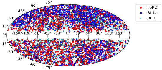
Figure 1.
Sky distribution of selected blazars in Hammer-Aitoff projection with Galactic coordinates.

Table 1.
Distribution of the number of blazar subclasses and their corresponding redshift (z) distributions.
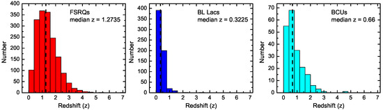
Figure 2.
Redshift distributions of FSRQs, BL Lacs, and BCUs in the sample. The black dashed lines indicate the median redshifts of the three subsamples.
To classify these blazars, we used three spectral energy distribution (SED) peak frequency () categories: LSP ( ≤ Hz), ISP ( Hz < < Hz), and HSP ( ≥ Hz) blazars. The peak frequencies were determined using data from Refs. [48,49,51] and the Open Universe for Blazars—Reference List V2.0 [52]5. Fermi blazars listed in the third catalog of AGNs detected by Fermi-LAT (3LAC) were initially classified based on their published values ([48]; Table 4, Column 9). The remaining Fermi blazars were classified using values from the fourth catalog of AGNs detected by Fermi-LAT (4LAC) ([49]; Table 3, column). For Fermi blazars lacking information in either catalog, and for all non-Fermi blazars, we first searched for potential data in the Open Universe for Blazars—Reference List V2.0. Finally, for sources without data in these references, we searched for potential data in Ref. [51]. This process resulted in the classification of 2264 LSPs, 512 ISPs, and 655 HSPs.
We generated 69,503 short-term light curves for all sources, averaging approximately 18 light curves per source. A representative long-term light curve for a BL Lac (5BZB J1135+3200 at z = 0.511) is presented in Figure 3, along with one of its short-term light curves. Among the final sample of 3816 blazars, 3806 sources had 3.4 m photometric data available from both the AllWISE and NEOWISE-R surveys, spanning a 13-year period from MJD 55203 to MJD 59926. The remaining 10 sources had 3.4 m photometric data solely from the NEOWISE-R survey, covering a 9-year period from MJD 56655 to MJD 59926.
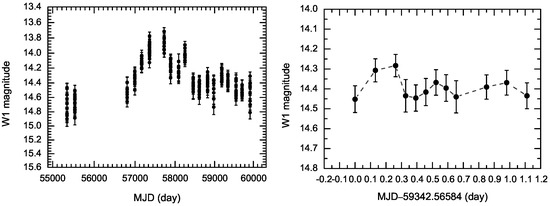
Figure 3.
Light curves of the BL Lac 5BZB J1135+3200 (z = 0.511) in the W1 band: (Left) long-term light curve; (Right) representative short-term light curve.
3. Methods and Results
3.1. Short-Term Variability Amplitude
A crucial aspect of blazar research involves investigating the amplitude of variability observed in their light curves. One of the most widely used metrics for this purpose is the intrinsic amplitude of variability () [53,54]. This parameter is derived by estimating the variance of the observed light curve after accounting for measurement errors. As described in Ref. [53], is calculated as follows:
where is the standard deviation of the light curve defined as
where N is the number of observations, is the ith magnitude, and is the weighted mean magnitude. The measurement uncertainty () incorporates both individual measurement errors and systematic uncertainty:
where represents the uncertainty associated with the ith magnitude and is the systematic uncertainty for the specific band. In the W1 band, the systematic uncertainty is 0.024 mag [55].
We computed the short-term variability amplitude () for each of the 69,503 short-term light curves using Equation (1). For each individual source, we selected the maximum value for further analysis. Ref. [46] calculated median values for different blazar subclasses by aggregating all short-term light curves within each subclass. Their approach provides a measure of the typical short-term variability for a given subclass. In contrast, our method focuses on identifying the maximum value for each individual source across multiple short-term light curves, followed by a comparative analysis of these maximum values across blazar subclasses.
The rms–flux correlation, a statistical relationship between the root-mean-square amplitude of variability and the average flux, has been observed in some blazars [56,57,58,59], suggesting that the source is more variable when it is brighter. Consistent with this correlation, maximum values are likely indicative of high-state activity. During these periods, increased jet turbulence or accretion disk fluctuations may contribute to higher brightness and greater variability. Conversely, quiescent or low states are characterized by reduced emission and variability due to a relatively stable jet and accretion disk. By analyzing maximum values, we aim to explore the upper limits of variability and complement the average variability analysis presented in [46]. A comparative analysis of both average and maximum distributions among various blazar subclasses offers a more nuanced understanding of the variability characteristics of blazars. For instance, one population of blazars might exhibit a similar distribution of average but a different distribution of maximum compared to another population of blazars.
The complete set of short-term values for all sources is provided in Table 2. Notably, only 23 blazars (∼0.6%) out of the 3816 have a short-term of zero, indicating a high prevalence of short-term MIR variability in this blazar population. The entire sample exhibits a range of short-term values from 0 mag to 1.636 mag, with a median of 0.149 mag. The distribution of short-term for the entire sample is presented in the left panel of Figure 4.
Table 2.
Classfication and MIR variability analysis results of our blazar sample .
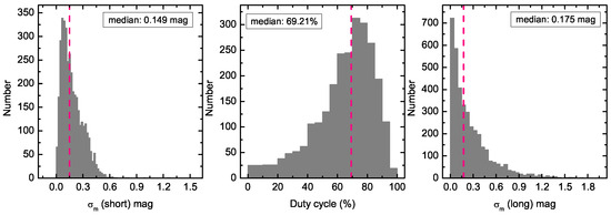
Figure 4.
Distributions of (Left) short-term variability amplitude quantified by , (Middle) duty cycle, and (Right) long-term variability amplitude quantified by for the entire sample. The pink dashed lines mark the median values of the data set.
We investigated the short-term distributions for different blazar subclasses (FSRQs vs. BL Lacs, Fermi vs. non-Fermi blazars, and LSPs vs. ISPs vs. HSPs). Figure 5 illustrates the normalized histograms, cumulative distribution functions (CDFs), and quantile–quantile (Q–Q) plots for each subclass. To indicate the 95% confidence interval in the CDF plots, we used the 2.5th and 97.5th percentiles of 1000 bootstrapped CDFs derived from the original data. In the Q–Q plots, a 45-degree line is included to visually compare the distributions of the two samples. The same visualization approach is used in Figure 6 and Figure 7.
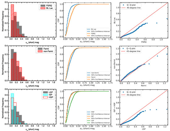
Figure 5.
Distributions of short-term for different subclasses of blazars. (Left) panels show normalized histograms. (Middle) panels display CDFs with 95% confidence intervals. (Right) panels present Q–Q plots, with red lines representing 45-degree lines.
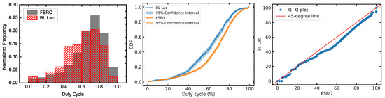
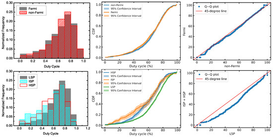
Figure 6.
Distributions of duty cycle (DC) for different subclasses of blazars. Left panels show normalized histograms. Middle panels display CDFs with 95% confidence intervals. Right panels present Q–Q plots, with red lines representing 45-degree lines.
Figure 7.
Distributions of long-term for different subclasses of blazars. (Left) panels show normalized histograms. (Middle) panels display CDFs with 95% confidence intervals. (Right) panels present Q–Q plots, with red lines representing 45-degree lines.
To determine if the short-term distributions of FSRQs and BL Lacs differ significantly, we conducted a k-sample Anderson–Darling test using the function within the SciPy scientific computing library [60,61]. The null hypothesis was that both distributions originate from the same source population. The k-sample Anderson–Darling test for FSRQs vs. BL Lacs resulted in a p-value < 0.0016. The median short-term values were mag for FSRQs and mag for BL Lacs, respectively. A k-sample Kruskal–Wallis test, using the function within the SciPy library, was employed to examine statistical differences between the medians of these groups [61,62]. The k-sample Kruskal–Wallis test yielded an H-statistic of 321.78 with a p-value of . Based on the H-statistic, we calculated the effect size using the formula = , where k is the number of groups and N is the total sample size. General guidelines for interpreting effect sizes in this context are as follows: < 0.01 indicates a negligible effect, 0.01 ≤ < 0.06 a small effect, 0.06 ≤ < 0.14 a medium effect, and ≥ 0.14 a large effect. The obtained was approximately 0.11, indicating a medium effect. The right-skewed distributions of short-term , as illustrated in Figure 5, necessitate an examination of the 75th and 95th percentiles to comprehend their shape and dispersion. For FSRQs, the 75th and 95th percentiles were 0.287 mag and 0.431 mag, respectively. For BL Lacs, these percentiles were 0.166 mag and 0.303 mag. These results collectively indicate statistically distinct short-term distributions between FSRQs and BL Lacs. Specifically, FSRQs exhibited significantly larger variability amplitudes on short time scales.
Figure 5 (middle panels, top to bottom) demonstrates a significant difference in the distributions of short-term between Fermi and non-Fermi blazars. A k-sample Anderson–Darling test resulted in a p-value less than 0.001, indicating statistically distinct distributions. The median short-term values were mag for Fermi blazars and mag for non-Fermi blazars, respectively. A k-sample Kruskal–Wallis test yielded an H-statistic of 78.83 with a p-value of . The calculated effect size was approximately 0.02, indicating a small effect. The 75th and 95th percentiles of the short-term distribution for Fermi blazars were 0.226 mag and 0.390 mag, respectively. For non-Fermi blazars, these percentiles were 0.280 mag and 0.420 mag. These results indicate statistically distinct short-term distributions between Fermi and non-Fermi blazars, with non-Fermi blazars exhibiting larger variability amplitudes on short time scales.
We further examined the short-term distributions for LSPs, ISPs, and HSPs. The bottom panels of Figure 5 suggest that the short-term distribution of LSPs differs from those of ISPs and HSPs, while ISPs and HSPs appear to have similar distributions. A k-sample Anderson–Darling test resulted in a p-value less than 0.001, indicating statistically distinct distributions. The median short-term values were mag, mag, for LSPs, ISPs, and HSPs, respectively. A k-sample Kruskal–Wallis test yielded an H-statistic of 353.32 with a p-value of . The calculated effect size was approximately 0.10, indicating a medium effect. We also calculated for pairwise Kruskal–Wallis tests. The results revealed a medium effect between LSPs and ISPs ( = 0.08), a medium effect between LSPs and HSPs ( = 0.07), and a negligible effect between ISPs and HSPs ( < 0.01). To identify specific groups that differed significantly in their short-term distributions, we conducted Dunn’s test as a post-hoc analysis following the Kruskal–Wallis test. Dunn’s test determines whether the differences between the medians of various groups are statistically significant, adjusting for multiple comparisons [63]. We employed the “Bonferroni” method to adjust the p-values, using the - Python package for efficient implementation of Dunn’s test7. The obtained adjusted p-values were for the comparison between LSPs and ISPs, for the comparison between LSPs and HSPs, and 0.41 for the comparison between ISPs and HSPs. In addition to comparing medians, we examined the 75th and 95th percentiles of the short-term distributions among LSPs, ISPs, and HSPs. For LSPs, the 75th and 95th percentiles were 0.284 mag and 0.427 mag, respectively. For ISPs, these percentiles were 0.157 mag and 0.298 mag. For HSPs, they were 0.170 mag and 0.300 mag. These results collectively suggest that LSPs exhibited significantly larger short-term compared to ISPs and HSPs, while ISPs and HSPs had comparable short-term values.
3.2. Duty Cycle
For each blazar in the sample, we obtained multiple short-term light curves, averaging approximately 18 per blazar. These light curves typically spanned ∼1–2 days. We used these data to estimate the duty cycle (DC) of short-term variability, defined as the fraction of time a source exhibits an active phase (flux exceeding a given threshold) or variability relative to the total observation period. This metric accounts for the fact that blazars may not display flux variations during all observational epochs. Following [64], the DC is calculated as
where is the redshift-corrected time interval of the jth light curve (), M is the number of short-term light curves for a given source, and is assigned a value of 1 for variable sources and 0 otherwise. Variability was determined using the criterion > 0 as outlined in Ref. [46]. We calculated the DC for 2567 blazars with known redshifts, as tabulated in Table 2. The overall DC distribution is shown in the middle panel of Figure 4. Only 19 blazars (∼0.5%) exhibited a DC of 0. The median DC for the sample was approximately 69.21%. These findings collectively indicate that blazars, as a population of AGNs, display frequent short-term variability.
To compare the distributions of DC among various blazar subclasses, we analyzed the 2567 sources with computed DC values. A k-sample Anderson–Darling test between FSRQs and BL Lacs resulted in a p-value less than 0.001, indicating statistically distinct distributions (see Figure 6, upper panels). FSRQs and BL Lacs exhibited median DC values of % and %, respectively. A k-sample Kruskal–Wallis test yielded an H-statistic of 51.63 with a p-value of . The calculated effect size was approximately 0.02, suggesting a small effect. As illustrated in Figure 6, the distributions of DC values exhibit a pronounced left-skewness. To gain a more nuanced understanding of their shapes and dispersions, it is essential to analyze the 5th and 25th percentiles. For FSRQs, the 5th and 25th percentiles of the DC distributions were 23.97% and 57.70%, respectively. For BL Lacs, these percentiles were 24.60% and 48.00%. These results demonstrate that FSRQs exhibited larger DC values compared to BL Lacs.
Figure 6 (middle panels, top to bottom) indicates that the DC distributions of Fermi and non-Fermi blazars are not significantly different. This finding was supported by a k-sample Anderson–Darling test, which yielded a p-value of 0.16. The median DC values for Fermi and non-Fermi blazars were % and %, respectively. A k-sample Kruskal–Wallis test resulted in an H-statistic of 0.63 with a p-value of . The calculated effect size was less than 0.01, suggesting a negligible effect. For Fermi blazars, the 5th and 25th percentiles of the DC distributions were 23.26% and 53.53%, respectively. For non-Fermi blazars, these percentiles were 23.88% and 55.80%. These findings suggest that there were no statistically significant disparities in the distributions of DC values between Fermi and non-Fermi blazars, and that their DC values were comparable.
The bottom panels of Figure 6 illustrate the DC distributions for LSPs, ISPs, and HSPs. A k-sample Anderson–Darling test revealed a p-value less than 0.001, indicating statistically distinct distributions among these subclasses. The median DC values are %, %, and % for LSPs, ISPs, and HSPs, respectively. A k-sample Kruskal–Wallis test yielded an H-statistic of 74.65 with a p-value of . The calculated effect size was approximately 0.03, suggesting a small effect. We also calculated for pairwise Kruskal–Wallis tests. The results revealed a small effect between LSPs and ISPs ( = 0.02), a small effect between LSPs and HSPs ( = 0.02), and a negligible effect between ISPs and HSPs ( < 0.01). Moreover, we conducted Dunn’s test as a post-hoc analysis following the Kruskal–Wallis test. The obtained adjusted p-values were for the comparison between LSPs and ISPs, for the comparison between LSPs and HSPs, and ≃1.0 for the comparison between ISPs and HSPs. In addition to comparing medians, we examined the 5th and 25th percentiles of the DC distributions among LSPs, ISPs, and HSPs. For LSPs, the 5th and 25th percentiles were 27.21% and 57.83%, respectively. For ISPs, these percentiles were 12.00% and 40.70%. For HSPs, they were 24.80% and 48.00%. These results jointly indicate that LSPs exhibited higher DC values compared to both ISPs and HSPs.
3.3. Long-Term Variability Amplitude
To investigate the long-term variability amplitude of selected blazars, we initially computed the mean MJD, W1 magnitude, and associated uncertainty for each observational epoch (typically spanning ∼1–2 days). This process generated a representative long-term light curve for each blazar. The weighted average W1 magnitude, , is computed as
where N is the number of photometric data points, represents the ith magnitude, is the weight, and denotes the uncertainty of . The standard error of the weighted average, as described in Ref. [65], is given by
We subsequently applied Equation (1) to determine the long-term for all blazars. The resulting values are presented in Table 2, and the overall distribution of long-term is depicted in the right panel of Figure 4. The median long-term for the sample was found to be 0.175 mag.
When comparing the long-term distributions between FSRQs and BL Lacs, a k-sample Anderson–Darling test resulted in a p-value less than 0.001, indicating statistically distinct distributions (see Figure 7, upper panels). FSRQs and BL Lacs exhibited median long-term of and , respectively. A k-sample Kruskal–Wallis test yielded an H-statistic of 0.06 with a p-value of 0.81. The calculated effect size was less than 0.01, suggesting a negligible effect. These results demonstrate that FSRQs and BL Lacs have different distributions of long-term , but their median values are similar. While their central tendencies are comparable, their overall shapes and spread vary. The normalized histograms reveal that FSRQs have a heavier tail. The CDFs plot shows a crossover between the two subclasses. The Q–Q plot further illustrates this difference: within the range of < 0.25 mag, the percentile points align with the 45-degree line, indicating similar distributions. However, within the range of > 0.25 mag, all points from FSRQs lie below the 45-degree line, suggesting that FSRQs tend to extend to larger values than BL Lacs. To quantify this difference, we computed the 75th and 95th percentiles of the long-term distributions for FSRQs and BL Lacs. The results were 0.383 mag and 0.306 mag for the 75th percentile, and 0.868 mag and 0.553 mag for the 95th percentile, respectively. If we adopt a more stringent criterion of 0.5 mag for long-term , 87 out of 1381 BL Lacs (∼6.8%) have a long-term value greater than 0.5 mag, while 305 out of 1740 FSRQs (∼17.5%) show a long-term larger than 0.5 mag. These findings collectively indicate that FSRQs tend to exhibit larger long-term values compared to BL Lacs.
Figure 7 (middle panels, top to bottom) presents a comparison of the long-term distributions for Fermi and non-Fermi blazars. A k-sample Anderson–Darling test revealed statistically significant differences between the two groups, with a p-value less than 0.001. Fermi blazars demonstrated a median long-term of , significantly higher than that of non-Fermi blazars, which had a median of . A k-sample Kruskal–Wallis test confirmed this disparity, yielding an H-statistic of 1083.58 with a p-value of . The calculated effect size was 0.28, suggesting a large effect. The 75th and 95th percentiles of the long-term distribution for Fermi blazars were 0.476 mag and 0.958 mag, respectively. For non-Fermi blazars, these percentiles were 0.147 mag and 0.378 mag. These findings indicate that Fermi blazars exhibited significantly larger long-term values compared to non-Fermi blazars.
Figure 7 (bottom panels) presents a comparison of the long-term distributions for LSPs, ISPs, and HSPs. A k-sample Anderson–Darling test yielded a p-value less than 0.001, indicating statistically distinct distributions among these subclasses. The median long-term values were , , and for LSPs, ISPs, and HSPs, respectively. A k-sample Kruskal–Wallis test yielded an H-statistic of 180.45 with a p-value of . The calculated effect size of approximately 0.05 indicates a small effect. We also calculated for pairwise Kruskal–Wallis tests. The results revealed a negligible effect between LSPs and ISPs ( < 0.01), a medium effect between LSPs and HSPs ( = 0.06), and a medium effect between ISPs and HSPs ( = 0.05). A post-hoc Dunn’s test revealed significant differences between LSPs and ISPs (adjusted p-value = ), LSPs and HSPs (adjusted p-value = ), and ISPs and HSPs (adjusted p-value = ). In addition to comparing medians, we examined the 75th and 95th percentiles of the long-term distributions among LSPs, ISPs, and HSPs. For LSPs, the 75th and 95th percentiles were 0.447 mag and 0.927 mag, respectively. For ISPs, these percentiles were 0.321 mag and 0.573 mag. For HSPs, they were 0.209 mag and 0.374 mag. These findings suggest that LSPs exhibited larger long-term values compared to both ISPs and HSPs.
To complement our analysis of long-term variability using , we employed the structure function (SF) to investigate variability behavior across different time scales. As a powerful, model-independent tool for empirically quantifying AGN variability, the SF measures the root-mean-square variability of sources. Given the sparse sampling of WISE data, we calculated the ensemble structure function (ESF) to characterize the average variability of different blazar subclasses [66]. Following Refs. [46,67], the ESF is defined as
where is the magnitude difference between two observations separated by a rest-frame time lag ( = , is a time lag in the observer frame), and is the sum of the squared uncertainties for these two magnitudes. To compute the SF for each blazar group, we binned the data using a 200-day (rest frame) step size for and calculated the average SF for each interval. Errors on SF were determined through error propagation as described in Refs. [46,67]. Figure 8 illustrates the SF for different blazar subclasses. Figure 8 presents the structure function (SF) as a function of time lag () for various blazar subclasses. A visual inspection of these plots reveals several key trends:
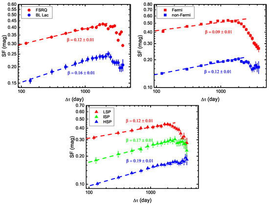
Figure 8.
Ensemble structure functions (ESFs) for blazar subclasses. ESFs are shown in the rest frame (log–log scale) for various blazar subclasses. Upper panels: Comparison of ESF between (left) FSRQs and BL Lacs, and (right) Fermi and non-Fermi blazars. (lower): Comparison of ESF among LSP, ISP, and HSP blazars. Dashed lines represent power-law fits to the ESFs (SF ∝ ) within the approximate range of 120 to 2000 days. Best-fit values are shown near the lines.
(i) All ESF curves exhibit a consistent profile characterized by an initial rise at shorter time lags followed by a plateau or gradual decline at longer time scales, a trend also observed in the studies of long-term quasar variability in the optical band (e.g., [67,68,69]). This suggests a common variability mechanism across blazar subclasses. Within the approximate range of 120 to 2000 days, a power-law increase (i.e., SF ∝, where is the power-law index) is evident for all blazar subclasses. The best-fit values for these subclasses range from 0.09 to 0.19, which are lower than the predicted value of 0.5 for the damped random walk (DRW) model, a stochastic model often used to describe the quasar variability [70]. This suggests that additional factors, such as relativistic beaming and intrinsic blazar properties, contribute to the observed values. A comparison of the best-fit values reveals that FSRQs exhibited a shallower ESF compared to BL Lacs, Fermi blazars exhibited a shallower ESF compared to BL Lacs, and LSPs exhibited a shallower ESF compared to ISPs and HSPs.
(ii) Within the approximate range of 120 to 3900 days, FSRQs exhibited higher ESF values than BL Lacs, indicating greater variability. Fermi blazars displayed more pronounced variability than non-Fermi blazars, as evidenced by their higher ESF values. A clear decreasing trend in ESF values was observed from LSPs to ISPs, and then to HSPs, suggesting that LSPs exhibited greater variability than both ISPs and HSPs. These ESF results are consistent with those obtained from long-term analysis.
4. Summary and Discussion
In this work we constructed a comprehensive dataset of 69,503 short-term 3.4 m (W1 band) light curves for 3816 blazars using WISE data spanning up to December 2022. Additionally, we derived a representative long-term 3.4 m light curve for each source through epoch averaging. A comparative analysis of short- and long-term intrinsic variability amplitude (), duty cycle (DC), and ensemble structure function (ESF) across blazar subclasses revealed significant differences in 3.4 m flux variability. Our findings are summarized as follows:
- FSRQs exhibited larger and DC values compared to BL Lacs.
- LSPs displayed larger and DC values relative to ISPs and HSPs.
- Fermi blazars demonstrated higher long-term but lower short-term relative to non-Fermi blazars, with similar DC distributions between the two groups.
- ESF analysis further confirmed the greater variability of FSRQs, LSPs, and Fermi blazars across a wide range of time scales compared to BL Lacs, ISPs/HSPs, and non-Fermi blazars.
Our study represents the most comprehensive statistical analysis of MIR variability among blazars to date. The observed significant disparity in MIR variability across blazar subclasses can be attributed to three primary factors: synchrotron peak frequency, jet power, and Doppler factor.
Within the standard leptonic emission model, W1 band emission is attributed to synchrotron radiation produced by a relativistic electron population with a broken power-law energy distribution [19]. The W1 band covers the declining portion of the synchrotron spectrum for LSPs, while it falls within the rising spectral region for HSPs and ISPs. Lower-energy electrons contribute to the rising synchrotron spectrum, whereas higher-energy particles produce the spectral decline. Given the inverse relationship between cooling time and electron energy (∝, where is the Lorentz factor of the electrons), high-energy electrons exhibit faster variability. Consequently, LSPs are anticipated to be more variable than HSPs and ISPs [71]. As the majority of FSRQs are classified as LSP sources and BL Lac objects as HSP sources, FSRQs are expected to be more variable compared to BL Lacs. Our findings are consistent with the leptonic emission scenario for blazar jets.
Disparities in jet power among blazar subclasses can also contribute to variability differences [46]. For instance, Ref. [72] found larger amplitude optical variability in FSRQs compared to BL Lacs, suggesting higher jet power in FSRQs as a potential cause for more substantial flares. Ref. [31] also found LSPs to be significantly more variable in the optical band than HSPs. The influence of higher jet power in FSRQs/LSPs can also explain the observed variability differences [73,74].
The relativistic Doppler boosting of the jet towards the observer plays a crucial role in non-thermal emission from blazars [4]. Consequently, Doppler effects can contribute to blazar variability. BL Lacs generally exhibit lower Doppler factors than FSRQs, potentially due to a selection bias favoring the detection of more FSRQs at higher redshifts (e.g., [75,76]). Additionally, non-Fermi blazars tend to have lower Doppler factors compared to Fermi blazars (e.g., [22,26]). These Doppler factor differences can also contribute to the observed variability disparities between blazar subclasses.
Fermi blazars exhibited larger long-term compared to non-Fermi blazars, while displaying lower short-term . This suggests distinct variability mechanisms dominating on short and long time scales. We propose that the higher Doppler factor in Fermi blazars relative to non-Fermi blazars primarily accounts for their larger long-term . An analysis of our Fermi and non-Fermi blazar samples revealed that non-Fermi blazars predominantly consist of LSPs (70.3%), while Fermi blazars have a lower LSP fraction (52.3%). This significant difference in LSP composition between the two groups likely explains the larger short-term observed in non-Fermi blazars relative to Fermi blazars.
This study extends previous studies of MIR variability in blazars [45,46]. Compared to previous studies with 2573 blazars [45] and 1035 Fermi blazars [46], this study encompasses a substantially larger sample of 3816 blazars. Furthermore, this study utilizes WISE data spanning approximately 13 years, significantly extending the temporal coverage of 4 and 7 years in Refs. [45,46]. In this study, an average of eighteen short-term light curves are collected per source, significantly exceeding the eight light curves per source obtained in the previous research by Ref. [46]. This increased dataset allows for a more comprehensive analysis of both short- and long-term variability across various blazar subclasses. Our findings corroborate previous results, including the higher long-term variability of Fermi blazars compared to non-Fermi blazars [45], and the greater variability of FSRQs compared to BL Lacs on both short and long time scales [46]. Additionally, we confirm previous findings [46] that LSP blazars exhibit higher variability than ISP and HSP blazars. This study presents, for the first time, a comparative analysis of short-term and DC distributions between Fermi and non-Fermi blazars, addressing a gap in previous investigations. Our results reveal that Fermi blazars exhibit lower short-term values compared to non-Fermi blazars, contrasting with the trend observed for long-term [45]. Our analysis indicates comparable DC values for Fermi and non-Fermi blazars. Contrary to the findings of Ref. [46], which identified BL Lacs as having higher DC values than FSRQs, our research observed the opposite trend. These new findings may provide valuable insights into the MIR variability properties of blazars.
Author Contributions
Conceptualization, X.Z. and L.M.; methodology, X.Z., Z.H. and L.M.; software, Z.H. and W.H.; validation, X.Z., Z.H. and L.M.; formal analysis, L.M.; investigation, L.M.; resources, X.Z., W.H. and L.M.; data curation, Z.H. and W.H.; writing—original draft preparation, X.Z.; writing—review and editing, X.Z. and L.M.; visualization, Z.H. and W.H.; supervision, X.Z. and L.M.; project administration, L.M.; funding acquisition, L.M. All authors have read and agreed to the published version of the manuscript.
Funding
This work is supported by the National Natural Science Foundation of China (Grant No. 12063007). L.M. acknowledges the Xingdian Talent Support Program of Yunnan Province.
Data Availability Statement
The original data presented in the study (i.e., complete Table 2) are openly available in the National Astronomical Data Center (NADC) of China, https://paperdata.china-vo.org/MLS/2024/Universe/Table2.csv, accessed on 24 July 2024.
Acknowledgments
We are grateful to the anonymous reviewers for their thoughtful comments and constructive suggestions, which significantly improved the quality of our manuscript. This work makes use of data products from the Wide-field Infrared Survey Explorer, which is a joint project of the University of California, Los Angeles, and the Jet Propulsion Laboratory/California Institute of Technology, funded by the National Aeronautics and Space Administration. This work also makes use of data products from NEOWISE, which is a project of the Jet Propulsion Laboratory/California Institute of Technology, funded by the Planetary Science Division of the National Aeronautics and Space Administration.
Conflicts of Interest
The authors declare no conflicts of interest.
Notes
| 1 | https://wise2.ipac.caltech.edu/docs/release/allwise, accessed on 10 December 2023. |
| 2 | https://wise2.ipac.caltech.edu/docs/release/neowise, accessed on 10 December 2023. |
| 3 | https://irsa.ipac.caltech.edu/, accessed on 21 December 2023. |
| 4 | https://wise2.ipac.caltech.edu/docs/release/allsky/expsup/sec2_4ci.html, accessed on 21 December 2023. |
| 5 | https://openuniverse.asi.it/OU4Blazars/MasterListV2/, accessed on 8 July 2023. |
| 6 | The p-values from the function are floored/capped at 0.001/0.25. |
| 7 | https://pypi.org/project/scikit-posthocs/, accessed on 23 August 2024. |
References
- Rees, M.J. Black Hole Models for Active Galactic Nuclei. Annu. Rev. Astron. Astrophys. 1984, 22, 471–506. [Google Scholar] [CrossRef]
- Antonucci, R. Unified models for active galactic nuclei and quasars. Annu. Rev. Astron. Astrophys. 1993, 31, 473–521. [Google Scholar] [CrossRef]
- Urry, C.M.; Padovani, P. Unified Schemes for Radio-Loud Active Galactic Nuclei. Publ. Astron. Soc. Pac. 1995, 107, 803. [Google Scholar] [CrossRef]
- Blandford, R.D.; Königl, A. Relativistic jets as compact radio sources. Astrophys. J. 1979, 232, 34–48. [Google Scholar] [CrossRef]
- Ackermann, M.; Anantua, R.; Asano, K.; Baldini, L.; Barbiellini, G.; Bastieri, D.; Becerra Gonzalez, J.; Bellazzini, R.; Bissaldi, E.; Blandford, R.D.; et al. Minute-timescale >100 MeV γ-Ray Variability during the Giant Outburst of Quasar 3C 279 Observed by Fermi-LAT in 2015 June. Astrophys. J. Lett. 2016, 824, L20. [Google Scholar] [CrossRef]
- Fan, J.H.; Kurtanidze, S.O.; Liu, Y.; Kurtanidze, O.M.; Nikolashvili, M.G.; Liu, X.; Zhang, L.X.; Cai, J.T.; Zhu, J.T.; He, S.L.; et al. Optical Photometry of the Quasar 3C 454.3 during the Period 2006–2018 and the Long-term Periodicity Analysis. Astrophys. J. Suppl. Ser. 2021, 253, 10. [Google Scholar] [CrossRef]
- Angelakis, E.; Hovatta, T.; Blinov, D.; Pavlidou, V.; Kiehlmann, S.; Myserlis, I.; Böttcher, M.; Mao, P.; Panopoulou, G.V.; Liodakis, I.; et al. RoboPol: The optical polarization of gamma-ray-loud and gamma-ray-quiet blazars. Mon. Not. R. Astron. Soc. 2016, 463, 3365–3380. [Google Scholar] [CrossRef]
- Aller, M.F.; Aller, H.D.; Hughes, P.A. Pearson-Readhead Survey Sources: Properties of the Centimeter-Wavelength Flux and Polarization of a Complete Radio Sample. Astrophys. J. 1992, 399, 16. [Google Scholar] [CrossRef]
- Liodakis, I.; Marscher, A.P.; Agudo, I.; Berdyugin, A.V.; Bernardos, M.I.; Bonnoli, G.; Borman, G.A.; Casadio, C.; Casanova, V.; Cavazzuti, E.; et al. Polarized blazar X-rays imply particle acceleration in shocks. Nature 2022, 611, 677–681. [Google Scholar] [CrossRef]
- Massaro, F.; Thompson, D.J.; Ferrara, E.C. The extragalactic gamma-ray sky in the Fermi era. Astron. Astrophys. Rev. 2015, 24, 2. [Google Scholar] [CrossRef]
- Pei, Z.Y.; Fan, J.H.; Bastieri, D.; Yang, J.H.; Xiao, H.B.; Yang, W.X. The relationship between the radio core-dominance parameter and spectral index in different classes of extragalactic radio sources (III). Res. Astron. Astrophys. 2020, 20, 025. [Google Scholar] [CrossRef]
- Stocke, J.T.; Morris, S.L.; Gioia, I.M.; Maccacaro, T.; Schild, R.; Wolter, A.; Fleming, T.A.; Henry, J.P. The Einstein Observatory Extended Medium-Sensitivity Survey. II. The Optical Identifications. Astrophys. J. Suppl. 1991, 76, 813. [Google Scholar] [CrossRef]
- Scarpa, R.; Falomo, R. Are high polarization quasars and BL Lacertae objects really different? A study of the optical spectral properties. Astron. Astrophys. 1997, 325, 109–123. [Google Scholar]
- Donato, D.; Ghisellini, G.; Tagliaferri, G.; Fossati, G. Hard X-ray properties of blazars. Astron. Astrophys. 2001, 375, 739–751. [Google Scholar] [CrossRef]
- Mao, L.S.; Xie, G.Z.; Bai, J.M.; Liu, H.T. Statistical Properties of a Blazar Sample and Comparison of HBLs, LBLs and FSRQs. Chin. J. Astron. Astrophys. 2005, 5, 471–486. [Google Scholar] [CrossRef]
- Ghisellini, G.; Tavecchio, F.; Foschini, L.; Ghirlanda, G. The transition between BL Lac objects and flat spectrum radio quasars. Mon. Not. R. Astron. Soc. 2011, 414, 2674–2689. [Google Scholar] [CrossRef]
- Fossati, G.; Maraschi, L.; Celotti, A.; Comastri, A.; Ghisellini, G. A unifying view of the spectral energy distributions of blazars. Mon. Not. R. Astron. Soc. 1998, 299, 433–448. [Google Scholar] [CrossRef]
- Mao, P.; Urry, C.M.; Massaro, F.; Paggi, A.; Cauteruccio, J.; Künzel, S.R. A Comprehensive Statistical Description of Radio-through-Gamma-Ray Spectral Energy Distributions of All Known Blazars. Astrophys. J. Suppl. Ser. 2016, 224, 26. [Google Scholar] [CrossRef]
- Böttcher, M.; Reimer, A.; Sweeney, K.; Prakash, A. Leptonic and Hadronic Modeling of Fermi-detected Blazars. Astrophys. J. 2013, 768, 54. [Google Scholar] [CrossRef]
- Abdo, A.A.; Ackermann, M.; Agudo, I.; Ajello, M.; Aller, H.D.; Aller, M.F.; Angelakis, E.; Arkharov, A.A.; Axelsson, M.; Bach, U.; et al. The Spectral Energy Distribution of Fermi Bright Blazars. Astrophys. J. 2010, 716, 30–70. [Google Scholar] [CrossRef]
- Ajello, M.; Baldini, L.; Ballet, J.; Bastieri, D.; Becerra Gonzalez, J.; Bellazzini, R.; Berretta, A.; Bissaldi, E.; Bonino, R.; Brill, A.; et al. The Fourth Catalog of Active Galactic Nuclei Detected by the Fermi Large Area Telescope: Data Release 3. Astrophys. J. Suppl. Ser. 2022, 263, 24. [Google Scholar] [CrossRef]
- Wu, Z.; Jiang, D.; Gu, M.; Chen, L. Why are some BL Lacertaes detected by Fermi, but others not? Astron. Astrophys. 2014, 562, A64. [Google Scholar] [CrossRef]
- Lister, M.L.; Aller, M.F.; Aller, H.D.; Hovatta, T.; Max-Moerbeck, W.; Readhead, A.C.S.; Richards, J.L.; Ros, E. Why Have Many of the Brightest Radio-loud Blazars Not Been Detected in Gamma-Rays by Fermi? Astrophys. J. Lett. 2015, 810, L9. [Google Scholar] [CrossRef]
- Deng, X.J.; Xue, R.; Wang, Z.R.; Xi, S.Q.; Xiao, H.B.; Du, L.M.; Xie, Z.H. The physical properties of γ-ray-quiet flat-spectrum radio quasars: Why are they undetected by Fermi-LAT? Mon. Not. R. Astron. Soc. 2021, 506, 5764–5773. [Google Scholar] [CrossRef]
- Xiong, D.; Zhang, X.; Bai, J.; Zhang, H. Basic properties of Fermi blazars and the ‘blazar sequence’. Mon. Not. R. Astron. Soc. 2015, 450, 3568–3578. [Google Scholar] [CrossRef]
- Savolainen, T.; Homan, D.C.; Hovatta, T.; Kadler, M.; Kovalev, Y.Y.; Lister, M.L.; Ros, E.; Zensus, J.A. Relativistic beaming and gamma-ray brightness of blazars. Astron. Astrophys. 2010, 512, A24. [Google Scholar] [CrossRef]
- Pushkarev, A.B.; Kovalev, Y.Y.; Lister, M.L.; Savolainen, T. Jet opening angles and gamma-ray brightness of AGN. Astron. Astrophys. 2009, 507, L33–L36. [Google Scholar] [CrossRef]
- Lister, M.L.; Homan, D.C.; Kadler, M.; Kellermann, K.I.; Kovalev, Y.Y.; Ros, E.; Savolainen, T.; Zensus, J.A. A Connection Between Apparent VLBA Jet Speeds and Initial Active Galactic Nucleus Detections Made by the Fermi Gamma-Ray Observatory. Astrophys. J. Lett. 2009, 696, L22–L26. [Google Scholar] [CrossRef]
- Piner, B.G.; Pushkarev, A.B.; Kovalev, Y.Y.; Marvin, C.J.; Arenson, J.G.; Charlot, P.; Fey, A.L.; Collioud, A.; Voitsik, P.A. Relativistic Jets in the Radio Reference Frame Image Database. II. Blazar Jet Accelerations from the First 10 Years of Data (1994–2003). Astrophys. J. 2012, 758, 84. [Google Scholar] [CrossRef]
- Pushkarev, A.B.; Kovalev, Y.Y. Single-epoch VLBI imaging study of bright active galactic nuclei at 2 GHz and 8 GHz. Astron. Astrophys. 2012, 544, A34. [Google Scholar] [CrossRef]
- Hovatta, T.; Pavlidou, V.; King, O.G.; Mahabal, A.; Sesar, B.; Dancikova, R.; Djorgovski, S.G.; Drake, A.; Laher, R.; Levitan, D.; et al. Connection between optical and γ-ray variability in blazars. Mon. Not. R. Astron. Soc. 2014, 439, 690–702. [Google Scholar] [CrossRef]
- Fuhrmann, L.; Angelakis, E.; Zensus, J.A.; Nestoras, I.; Marchili, N.; Pavlidou, V.; Karamanavis, V.; Ungerechts, H.; Krichbaum, T.P.; Larsson, S.; et al. The F-GAMMA programme: Multi-frequency study of active galactic nuclei in the Fermi era. Programme description and the first 2.5 years of monitoring. Astron. Astrophys. 2016, 596, A45. [Google Scholar] [CrossRef]
- Bhatta, G.; Webb, J. Microvariability in BL Lacertae: “Zooming” into the Innermost Blazar Regions. Galaxies 2018, 6, 2. [Google Scholar] [CrossRef]
- Wagner, S.J.; Witzel, A. Intraday Variability In Quasars and BL Lac Objects. Annu. Rev. Astron. Astrophys. 1995, 33, 163–198. [Google Scholar] [CrossRef]
- Gupta, A.C.; Fan, J.H.; Bai, J.M.; Wagner, S.J. Optical Intra-Day Variability in Blazars. Astron. J. 2008, 135, 1384–1394. [Google Scholar] [CrossRef]
- Sandrinelli, A.; Covino, S.; Treves, A. Long and short term variability of seven blazars in six near-infrared/optical bands. Astron. Astrophys. 2014, 562, A79. [Google Scholar] [CrossRef]
- Fan, J.H.; Xie, G.Z.; Pecontal, E.; Pecontal, A.; Copin, Y. Historic Light Curve and Long-Term Optical Variation of BL Lacertae 2200 + 420. Astrophys. J. 1998, 507, 173–178. [Google Scholar] [CrossRef]
- Villforth, C.; Nilsson, K.; Heidt, J.; Takalo, L.O.; Pursimo, T.; Berdyugin, A.; Lindfors, E.; Pasanen, M.; Winiarski, M.; Drozdz, M.; et al. Variability and stability in blazar jets on time-scales of years: Optical polarization monitoring of OJ 287 in 2005–2009. Mon. Not. R. Astron. Soc. 2010, 402, 2087–2111. [Google Scholar] [CrossRef]
- Bonning, E.; Urry, C.M.; Bailyn, C.; Buxton, M.; Chatterjee, R.; Coppi, P.; Fossati, G.; Isler, J.; Maraschi, L. SMARTS Optical and Infrared Monitoring of 12 Gamma-Ray Bright Blazars. Astrophys. J. 2012, 756, 13. [Google Scholar] [CrossRef]
- Safna, P.Z.; Stalin, C.S.; Rakshit, S.; Mathew, B. Long-term optical and infrared variability characteristics of Fermi blazars. Mon. Not. R. Astron. Soc. 2020, 498, 3578–3591. [Google Scholar] [CrossRef]
- Gupta, A.C.; Kushwaha, P.; Carrasco, L.; Xu, H.; Wiita, P.J.; Escobedo, G.; Porras, A.; Recillas, E.; Mayya, Y.D.; Chavushyan, V.; et al. Long-term Multiband Near-infrared Variability of the Blazar OJ 287 during 2007–2021. Astrophys. J. Suppl. Ser. 2022, 260, 39. [Google Scholar] [CrossRef]
- Wright, E.L.; Eisenhardt, P.R.M.; Mainzer, A.K.; Ressler, M.E.; Cutri, R.M.; Jarrett, T.; Kirkpatrick, J.D.; Padgett, D.; McMillan, R.S.; Skrutskie, M.; et al. The Wide-field Infrared Survey Explorer (WISE): Mission Description and Initial On-orbit Performance. Astron. J. 2010, 140, 1868–1881. [Google Scholar] [CrossRef]
- Mainzer, A.; Bauer, J.; Grav, T.; Masiero, J.; Cutri, R.M.; Dailey, J.; Eisenhardt, P.; McMillan, R.S.; Wright, E.; Walker, R.; et al. Preliminary Results from NEOWISE: An Enhancement to the Wide-field Infrared Survey Explorer for Solar System Science. Astrophys. J. 2011, 731, 53. [Google Scholar] [CrossRef]
- Mainzer, A.; Bauer, J.; Cutri, R.M.; Grav, T.; Masiero, J.; Beck, R.; Clarkson, P.; Conrow, T.; Dailey, J.; Eisenhardt, P.; et al. Initial Performance of the NEOWISE Reactivation Mission. Astrophys. J. 2014, 792, 30. [Google Scholar] [CrossRef]
- Mao, L.; Zhang, X.; Yi, T. Mid-infrared variability of blazars: A view from NEOWISE survey. Astrophys. Space Sci. 2018, 363, 167. [Google Scholar] [CrossRef]
- Anjum, A.; Stalin, C.S.; Rakshit, S.; Gudennavar, S.B.; Durgapal, A. Mid-infrared variability of γ-ray emitting blazars. Mon. Not. R. Astron. Soc. 2020, 494, 764–774. [Google Scholar] [CrossRef]
- Massaro, E.; Giommi, P.; Leto, C.; Marchegiani, P.; Maselli, A.; Perri, M.; Piranomonte, S.; Sclavi, S. Roma-BZCAT: A multifrequency catalogue of blazars. Astron. Astrophys. 2009, 495, 691–696. [Google Scholar] [CrossRef]
- Ackermann, M.; Ajello, M.; Atwood, W.B.; Baldini, L.; Ballet, J.; Barbiellini, G.; Bastieri, D.; Becerra Gonzalez, J.; Bellazzini, R.; Bissaldi, E.; et al. The Third Catalog of Active Galactic Nuclei Detected by the Fermi Large Area Telescope. Astrophys. J. 2015, 810, 14. [Google Scholar] [CrossRef]
- Ajello, M.; Angioni, R.; Axelsson, M.; Ballet, J.; Barbiellini, G.; Bastieri, D.; Becerra Gonzalez, J.; Bellazzini, R.; Bissaldi, E.; Bloom, E.D.; et al. The Fourth Catalog of Active Galactic Nuclei Detected by the Fermi Large Area Telescope. Astrophys. J. 2020, 892, 105. [Google Scholar] [CrossRef]
- Rakshit, S.; Johnson, A.; Stalin, C.S.; Gandhi, P.; Hoenig, S. WISE view of narrow-line Seyfert 1 galaxies: Mid-infrared colour and variability. Mon. Not. R. Astron. Soc. 2019, 483, 2362–2370. [Google Scholar] [CrossRef]
- Kudryavtsev, D.O.; Sotnikova, Y.V.; Stolyarov, V.A.; Mufakharov, T.V.; Vlasyuk, V.V.; Khabibullina, M.L.; Mikhailov, A.G.; Cherepkova, Y.V. Cluster Analysis of the Roma-BZCAT Blazars. Res. Astron. Astrophys. 2024, 24, 055011. [Google Scholar] [CrossRef]
- Giommi, P.; Brandt, C.H.; Barres de Almeida, U.; Pollock, A.M.T.; Arneodo, F.; Chang, Y.L.; Civitarese, O.; De Angelis, M.; D’Elia, V.; Del Rio Vera, J.; et al. Open Universe for Blazars: A new generation of astronomical products based on 14 years of Swift-XRT data. Astron. Astrophys. 2019, 631, A116. [Google Scholar] [CrossRef]
- Sesar, B.; Ivezić, Ž.; Lupton, R.H.; Jurić, M.; Gunn, J.E.; Knapp, G.R.; DeLee, N.; Smith, J.A.; Miknaitis, G.; Lin, H.; et al. Exploring the Variable Sky with the Sloan Digital Sky Survey. Astron. J. 2007, 134, 2236–2251. [Google Scholar] [CrossRef]
- Ai, Y.L.; Yuan, W.; Zhou, H.Y.; Wang, T.G.; Dong, X.B.; Wang, J.G.; Lu, H.L. Dependence of the Optical/Ultraviolet Variability on the Emission-line Properties and Eddington Ratio in Active Galactic Nuclei. Astrophys. J. Lett. 2010, 716, L31–L35. [Google Scholar] [CrossRef]
- Jarrett, T.H.; Cohen, M.; Masci, F.; Wright, E.; Stern, D.; Benford, D.; Blain, A.; Carey, S.; Cutri, R.M.; Eisenhardt, P.; et al. The Spitzer-WISE Survey of the Ecliptic Poles. Astrophys. J. 2011, 735, 112. [Google Scholar] [CrossRef]
- Kundu, A.; Chatterjee, R.; Mitra, K.; Mondal, S. rms-flux relation and disc-jet connection in blazars in the context of the internal shocks model. Mon. Not. R. Astron. Soc. 2022, 510, 3688–3700. [Google Scholar] [CrossRef]
- Giebels, B.; Degrange, B. Lognormal variability in BL Lacertae. Astron. Astrophys. 2009, 503, 797–799. [Google Scholar] [CrossRef]
- Kushwaha, P.; Sinha, A.; Misra, R.; Singh, K.P.; de Gouveia Dal Pino, E.M. Gamma-Ray Flux Distribution and Nonlinear Behavior of Four LAT Bright AGNs. Astrophys. J. 2017, 849, 138. [Google Scholar] [CrossRef]
- Bhatta, G. Characterizing Long-term Optical Variability Properties of γ-Ray-bright Blazars. Astrophys. J. 2021, 923, 7. [Google Scholar] [CrossRef]
- Scholz, F.W.; Stephens, M.A. K-sample Anderson–Darling tests. J. Am. Stat. Assoc. 1987, 82, 918–924. [Google Scholar]
- Virtanen, P.; Gommers, R.; Oliphant, T.E.; Haberland, M.; Reddy, T.; Cournapeau, D.; Burovski, E.; Peterson, P.; Weckesser, W.; Bright, J.; et al. SciPy 1.0: Fundamental algorithms for scientific computing in Python. Nat. Methods 2020, 17, 261–272. [Google Scholar] [CrossRef]
- Kruskal, W.H.; Wallis, W.A. Use of ranks in one-criterion variance analysis. J. Am. Stat. Assoc. 1952, 47, 583–621. [Google Scholar] [CrossRef]
- Dunn, O.J. Multiple comparisons using rank sums. Technometrics 1964, 6, 241–252. [Google Scholar] [CrossRef]
- Romero, G.E.; Cellone, S.A.; Combi, J.A. Optical microvariability of southern AGNs. Astron. Astrophys. Suppl. 1999, 135, 477–486. [Google Scholar] [CrossRef]
- Bevington, P.R. Data Reduction and Error Analysis for the Physical Sciences; McGraw-Hill Education: New York, NY, USA, 1969. [Google Scholar]
- Emmanoulopoulos, D.; McHardy, I.M.; Uttley, P. On the use of structure functions to study blazar variability: Caveats and problems. Mon. Not. R. Astron. Soc. 2010, 404, 931–946. [Google Scholar] [CrossRef]
- Vanden Berk, D.E.; Wilhite, B.C.; Kron, R.G.; Anderson, S.F.; Brunner, R.J.; Hall, P.B.; Ivezić, Ž.; Richards, G.T.; Schneider, D.P.; York, D.G.; et al. The Ensemble Photometric Variability of ∼25,000 Quasars in the Sloan Digital Sky Survey. Astrophys. J. 2004, 601, 692–714. [Google Scholar] [CrossRef]
- Gallastegui-Aizpun, U.; Sarajedini, V.L. The ensemble optical variability of type-1 AGN in the Sloan Digital Sky Survey Data Release 7. Mon. Not. R. Astron. Soc. 2014, 444, 3078–3088. [Google Scholar] [CrossRef]
- Kozłowski, S. Revisiting Stochastic Variability of AGNs with Structure Functions. Astrophys. J. 2016, 826, 118. [Google Scholar] [CrossRef]
- Kelly, B.C.; Bechtold, J.; Siemiginowska, A. Are the Variations in Quasar Optical Flux Driven by Thermal Fluctuations? Astrophys. J. 2009, 698, 895–910. [Google Scholar] [CrossRef]
- Paliya, V.S.; Stalin, C.S.; Ajello, M.; Kaur, A. Intra-night Optical Variability Monitoring of Fermi Blazars: First Results from 1.3 m J. C. Bhattacharya Telescope. Astrophys. J. 2017, 844, 32. [Google Scholar] [CrossRef]
- Bauer, A.; Baltay, C.; Coppi, P.; Ellman, N.; Jerke, J.; Rabinowitz, D.; Scalzo, R. Blazar Optical Variability in the Palomar-Quest Survey. Astrophys. J. 2009, 699, 1732–1741. [Google Scholar] [CrossRef]
- Gardner, E.; Done, C. What powers the most relativistic jets?-I. BL Lacs. Mon. Not. R. Astron. Soc. 2014, 438, 779–788. [Google Scholar] [CrossRef]
- Gardner, E.; Done, C. What powers the most relativistic jets?-II. Flat-spectrum radio quasars. Mon. Not. R. Astron. Soc. 2018, 473, 2639–2654. [Google Scholar] [CrossRef]
- Lister, M.L.; Aller, M.F.; Aller, H.D.; Homan, D.C.; Kellermann, K.I.; Kovalev, Y.Y.; Pushkarev, A.B.; Richards, J.L.; Ros, E.; Savolainen, T. MOJAVE. X. Parsec-scale Jet Orientation Variations and Superluminal Motion in Active Galactic Nuclei. Astron. J. 2013, 146, 120. [Google Scholar] [CrossRef]
- Liodakis, I.; Pavlidou, V. Population statistics of beamed sources-I. A new model for blazars. Mon. Not. R. Astron. Soc. 2015, 451, 2434–2446. [Google Scholar] [CrossRef][Green Version]


Disclaimer/Publisher’s Note: The statements, opinions and data contained in all publications are solely those of the individual author(s) and contributor(s) and not of MDPI and/or the editor(s). MDPI and/or the editor(s) disclaim responsibility for any injury to people or property resulting from any ideas, methods, instructions or products referred to in the content. |
© 2024 by the authors. Licensee MDPI, Basel, Switzerland. This article is an open access article distributed under the terms and conditions of the Creative Commons Attribution (CC BY) license (https://creativecommons.org/licenses/by/4.0/).