Abstract
The objective of this paper is to reproduce and predict the series of solar cycle amplitudes using a simple time-series model that takes into account the variable time scale of the Gleissberg oscillation and the absence of clear evidence for odd–even alternation prior to Solar Cycle 9 (SC9). It is demonstrated that the Gleissberg oscillation can be quite satisfactorily modelled as a sinusoidal variation of constant amplitude with a period increasing linearly with time. Subtracting this model from the actual cycle amplitudes, a clear even–odd alternating pattern is discerned in the time series of the residuals since SC9. For this period of time, the mean value of the residuals for odd-numbered cycles is shown to exceed the value for even-numbered cycles by more than , providing the clearest evidence yet for a persistent odd–even–odd alternation in cycle amplitudes. Random deviations from these means are less than half the standard deviation of the raw cycle amplitude time series for the same period, which allows the use of these regularities for solar cycle prediction with substantially better confidence than the simple climatological average. Predicted cycle amplitudes are found to be robust against the addition or omission of some data points from the input set, and the method correctly hindcasts SC23 and SC24. The potential physical background of the regularities is also discussed. Our predictions for the amplitudes of SC25, SC26, and SC27 are , and , respectively. This suggests that the amplitude of SC26 will be even lower than that of SC24, making it the weakest cycle since the Dalton Minimum.
1. Introduction
Regularities in the long-term variation of solar activity have long been sought and found. A 22-year cyclicity, evident in the frequently observed alternation in the amplitudes of subsequent cycles, was noted early on (see [1]). In 1939, Gleissberg [2] called attention to an oscillatory signal with a period of about eight solar cycles. Terrestrial proxy records indicate the existence of even longer periodicities in solar activity [3,4].
Attempts to exploit these oscillatory variations for solar cycle prediction have, however, not met with much success [5]. The underlying cause of this, as already recognised by Gleissberg [6], is that apparent periodicities found by harmonic analysis may vary or vanish with time, and depend on the reference period of time for which they are derived. Specifically, the odd–even alternation may have been absent and/or have passed through a phase jump during and before the Dalton Minimum [7], while the time scale of the Gleissberg oscillation has been shown to be steadily increasing since the 18th century [8,9]. As these shorter time scale variations are the most relevant for cycle prediction, precursor methods and physical model-based approaches have largely superseded time-series methods in the field.
In this paper, a new attempt is made at reproducing and predicting the series of solar cycle amplitudes using a simple model that takes into account the variable time scale of the Gleissberg oscillation and the absence of clear evidence for odd–even alternation prior to Solar Cycle 9 (SC9). Random deviations from this model are found to be less than half the standard deviation of the raw cycle amplitude time series for the same period, which allows the use of these regularities for solar cycle prediction with substantially better confidence than the simple climatological average.
2. Data and Methods
International sunspot numbers (version 2), provided by World Data Center for Sunspot Index and Long-term Solar Observations (WDC-SILSO) of the Solar Influences Data Analysis Center (SIDC) at the Royal Observatory of Belgium, were used for this study [10]. Following general practice in solar physics, cycle maxima were defined by the maxima of the 13-month smoothed value of the international sunspot number, . Integrated cycle amplitudes were calculated as the sum of the yearly mean total sunspot numbers during a cycle, with the minimum years counted to the incipient cycle. The resulting cycle amplitude parameters are given in the Supplementary data.
Nonlinear parameter fitting was performed with the Levenberg–Marquardt algorithm, as implemented in the scipy.optimize.curve_fit function of Python 3.10.
3. Analysis and Results
Following the standard approach in Gleissberg’s work [11,12], for the study of centennial-scale variations in the amplitude of solar activity, shorter variations are filtered out by taking a boxcar average of cycle amplitudes with weight 12221. The amplitude of cycle n filtered is then given by:
This smoothed variation is here fitted with a sinusoidal of constant amplitude and linearly increasing period, i.e.,
The best fit is displayed in Figure 1 in green dash-dots. With a mean error (relative to the curve amplitude) of ∼7% only, the fit is quite convincing (, ). A fit with a constant period (), in contrast, leads to a mean error of 18% with , and a p value of 0.114 only. (Note that an exponentially increasing period was also tested, but the fit was found to be inferior to the linear case.)
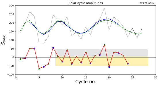
Figure 1.
Solar cycle maximum amplitudes. The raw maximum amplitudes are shown in light grey; 12221 filtered values in blue. An analytic fit with a sinusoidal variation of linearly increasing period is shown by the green dash-dotted line. Residuals obtained by subtracting the fit from the raw data are displayed in red in the lower part of the figure. From SC9, a systematic shift between odd-numbered (green triangles) and even-numbered (blue dots) cycles is clearly visible; bands of width around the respective mean values of the residuals for odd and even cycles are shown in grey and gold, respectively. The dashed extension of the light grey curve presents the prediction of upcoming sunspot cycles based on these regularities.
Subtracting the fitted values from the raw, unsmoothed cycle amplitudes results in the residuals plotted in red in the lower part of the figure. A characteristic, persistent zig-zag pattern of alternating amplitudes is apparent, especially starting from SC9. Prior to that time, issues arise with the coverage and homogeneity of observations, as well as with the atypical behaviour of the Sun itself around the Dalton minimum [13,14], so here we will focus on cycles starting from SC9. The mean value of the residual for odd and even cycles in this period are and , respectively, which yields a difference. This is the strongest statistical evidence yet for a systematic difference between even and odd cycle amplitudes, made possible by the subtraction of the linearly lengthening Gleissberg oscillation.
For individual cycles, the residual amplitudes scatter around the mean, with a standard deviation of 21.205 and 26.061 for odd and even cycles, respectively. This is an improvement to a factor of two relative to the scatter of 47.233 shown by all cycles around the climatological average amplitude for the same period. Hence, adding the mean value of the residual that corresponds to the odd/even cycle number to our model, as seen in Equation (2), for the Gleissberg oscillation offers a way to predict the amplitudes of solar cycles with substantially better precision than simple climatology. These predictions are shown by the dashed line in Figure 1 and subsequent figures.
As the procedure involves a nonlinear parameter optimization routine, questions may arise as to how stable it is in response to the addition or omission of a few data points. To test this, in Figure 2, we present a “hindcast” produced using data up to SC22 only. This results in a “postdiction” for SC23 and SC24. The predicted values are and , which compare favourably with the observed values of 180.3 and 116.4, respectively.
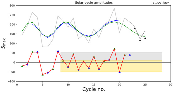
Figure 2.
Solar cycle maximum amplitudes considering data up to SC22 only. Asterisks mark the observed maximum amplitudes of SC23 and SC24, while the black triangle is the current lower estimate for SC25, to be compared with the predictions. For other notations see the caption of Figure 1.
A disadvantage of the 12221 filtering is that it lags behind the most recent cycle by two cycles. A 121 filter of the form
is expected to give more weight to the recent variation in solar activity, potentially leading to improved predictions. Indeed, a hindcast using 121 filtering (Figure 3) leads to further improved postdictions for SC23 and SC24, at 181.9 and 113.1, respectively.
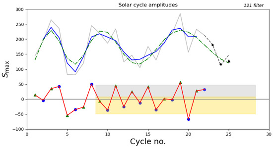
Figure 3.
Solar cycle maximum amplitudes considering data up to SC22 only, with a 121 filter used for smoothing. Asterisks mark the observed maximum amplitudes of SC23 and SC24, while the black triangle is the current lower estimate for SC25, to be compared with the predictions. For other notations see the caption of Figure 1.
Prompted by this improvement, for our “official” forecast, we use all data available up to SC24 and a 121 filter (Figure 4). Parameters for the optimised fit are , , , , and . Odd (even) cycles scatter around a value offset by +23.6 (−24.2) relative to this fit, with a standard deviation of 20.7 (25.1).
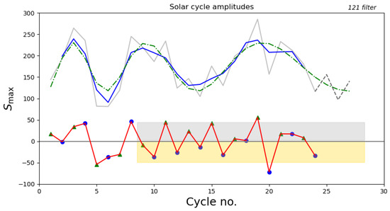
Figure 4.
Solar cycle maximum amplitudes considering all numbered cycles, with a 121 filter used for smoothing. For notations see the caption of Figure 1.
The resulting predictions for SC25, SC26, and SC27 are , and , respectively. This suggests that SC26 will be even lower in amplitude than SC24 was, making it the weakest cycle since the Dalton Minimum.
Current predictions for SC25 by SILSO and the SWPC tend to fall below our prediction here: they typically fall in the range of 128–154, though the full range covered extends from 100 to 171 [15,16,17,18,19]. Should this cycle indeed prove to be a negative fluke exceeding , how would that impact on the further predictions for the forthcoming cycles? To test this, we also compute fiducial forecasts including fiducial data for SC25, assuming that its amplitude will not exceed the current lower limit of 127.1 (reached in November 2023). The outcomes from our various models are summarised in Table 1. It is apparent that predictions are quite robust against minor changes in the input data set, leaving our above conclusion about SC26 intact. The use of a 12221 filter invariably leads to somewhat higher predictions, but still within the limit.

Table 1.
Predictions for solar cycles from different choices of input data and smoothing. Bold numbers denote preferred values. Numbers in italics are input values. All numbers were rounded to integers for brevity.
Beside their maximum amplitude, another measure of solar cycles is their integrated sunspot area, i.e., the sum of annual mean sunspot numbers during their whole duration (area under the curve). Indeed, the odd–even alternation is often seen more evidently in these data [7,20]. Repeating the fitting exercises outlined above for , our findings are similar. An example case is shown in Figure 5. While the results of the “hindcast” test (see Table 1) are somewhat less convincing in the data, the odd–even alternation is now even more consistently seen in the residuals, without a single exception since SC9.
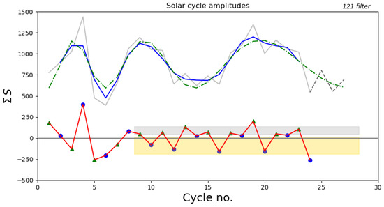
Figure 5.
Solar cycle integrated sunspot areas with a 121 filter used for smoothing. For other notations see the caption of Figure 1.
4. Discussion
The convincing forecasting performance of the simple time-series model presented above, based on a combination of a secular oscillation with linearly increasing amplitude and an odd–even alternation, calls for a theoretical interpretation.
4.1. Gleissberg Oscillation
In oscillatory phenomena like the solar dynamo, long-period secondary oscillations often arise as a beat period due to a second base period. As the beat frequency equals the difference of the base frequencies, a century-scale oscillation might be interpreted as the beat of two base periods separated by ∼1 year. For example, two base cycle periods of 10.5 and 11.5 years would yield a beat period of 10 cycles, comparable to the Gleissberg cycle.
In the currently prevailing Babcock–Leighton type dynamo models, the cycle period is determined by the speed of the meridional flow, which is most commonly assumed to be single-celled. In such a situation, two different base periods can only be present if the meridional flow amplitude differs between the northern and southern hemispheres. Furthermore, if hemispheric coupling reduces this flow difference, the two periods will approach each other, and the beat period will increase. A simple(-minded?) explanation for the linearly lengthening Gleissberg oscillation would then assume a ∼20% initial difference in the meridional flow in the early 18th century, followed by a gradual reduction over the subsequent three centuries. One may speculate that this initial hemispheric asymmetry at the end of the Maunder Minimum could potentially be related to the extreme hemispheric asymmetry of the (low) solar activity during the Maunder Minimum, when nearly all sunspots were observed on the southern hemisphere.
The coupling between the meridional circulation cells in the two hemispheres occurs via turbulent viscous stress in the equatorial plane. For simplicity, let us ignore the details of the meridional flow pattern, and assume simply that the momentum density is initially constant throughout the volume of each hemisphere, with a jump across the equator. As the equatorial stress is , where is the turbulent viscosity and x is the latitudinal coordinate, the problem is simplified to solving a 1D diffusion equation:
The step function initial condition is as follows:
The solution reads:
Within the finite volume of the convective zone, of horizontal extent ∼R, where R is the solar radius, the hemispheric meridional flow momentum excess/deficit can then be estimated as:
Using R as the unit of length and as the unit of time, the integral evaluates to:
As the difference in flow amplitude scales with D, so does the difference in the frequency of the dynamo cycles. Hence, the beat period will scale with the inverse of D. This function is plotted in Figure 6. Note that our time unit translates to:
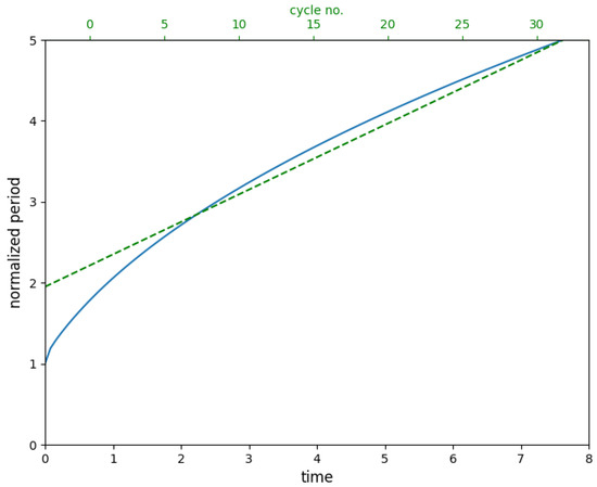
Figure 6.
Normalised beat period (blue solid) against nondimensional time for the 1D interhemispheric relaxation. The cycle numbering at the top axis assumes a turbulent viscosity km2s. The green dashed line is Equation (2) with our best fit parameters.
It is apparent from the figure that, when normalised to a similar level, the predicted variation of the beat period is comparable to the observed Gleissberg variation for a turbulent viscosity value of km2s, considered realistic in the solar convective zone. These findings then suggest that the cause of the Gleissberg oscillation with a nearly linearly increasing period is the still ongoing inter-hemispheric relaxation of the meridional circulation as a closing act of the Maunder Minimum or of the entire Spörer episode.
A number of caveats exist regarding the scenario outlined above.
Firstly, in contrast to the angular momentum (momentum of the rotational flow), the momentum of the meridional circulation is not conserved. Hence, boundary stresses are not the only factor in its variation. The main internal generation terms involve nondiagonal terms in the Reynolds stress tensor. As the amplitude of these terms is expected to remain below the amplitude of the diagonal terms in most of the convective zone, their neglect in our rough calculation above may be acceptable to a first approximation.
Secondly, observations show major spatio-temporal fluctuations in the meridional flow on timescales of a few months. This, however, plausibly involves an internal reorganization of the flow pattern only, without a significant change in the total momentum of the flow integrated over a hemisphere, again leaving the main conclusion above intact.
Finally, the underlying concept of a beat of two oscillations assumes that the two hemispheres behave as independent oscillators with two different periods. Intuitively, while this may be conceivable for the quadrupole dynamo mode, it is hardly possible for the dominant dipole mode, due to the strong magnetic link between the hemispheres. Hence, for the beat to be associated with a significant amplitude modulation, some kind of nonlinearity is needed in the model, coupling the modes and allowing the beat in the quadrupole mode to imprint on the dipole mode. As the quadrupole term is responsible for hemispheric asymmetry in the large-scale magnetic field, its role is supported by the fact that the Gleissberg oscillation has been found to be associated with hemispheric asymmetry patterns in a number of studies [8,21].
Despite its attractive features, it is important to realise that the explanation of the Gleissberg oscillation and its time variation proposed here is not unique. A number of other explanations for the oscillation have been suggested [22,23,24], even though the possibility of their regular period variation has not been explored to date. In particular, the mechanism proposed in [25], relying on magnetic feedback in the differential rotation, shows some parallels to our proposal. Another parallel is the proposal that a beat between the dipole mode and the (unstable or stochastically excited) quadrupole mode is responsible for longer periodicities related to hemispheric asymmetries [26,27].
4.2. Odd–Even Alternation
The other main element of the prediction method applied here, the systematic odd–even alternation, does not require new hypotheses as such alternation, persisting for long periods of time, is regularly seen in many nonlinear dynamo models [28,29,30].
The origin of this behaviour is readily understood in terms of a nonlinear solar dynamo [31,32,33]. For a relatively broad class of nonlinearities, dynamo models above a second (not necessarily very high) critical dynamo number may undergo a Hopf bifurcation with period doubling. Even in the absence of an unstable period-2 mode, the oscillatory character of the return to a stable base period can induce alternating behaviour in the presence of stochastic forcing.
The bad news is that in stochastically perturbed models, the length of persistent alternating sequences is unpredictable, following a power law distribution. There is no known way to tell in advance when such a sequence will end. This constitutes the main limitation of our method, not reflected in the formal error range: there is no guarantee that the ongoing persistent sequence of odd–even alternation will not suddenly end due to stochastic fluctuations like rogue active regions [34,35].
A time-honoured alternative explanation for cycle alternation is the presence of a relic magnetic field in the deep solar interior that adds to or reduces the amplitude of magnetic cycles, depending on their polarity [36]. Evidence for this has been claimed on the basis of hemispheric asymmetries [37]. As in this case no phase jumps are expected in the alternation, this eventuality would actually reduce the uncertainty in our prediction.
5. Conclusions
In this paper, a new attempt was made at reproducing and predicting the series of solar cycle amplitudes using a simple model that takes into account the variable time scale of the Gleissberg oscillation and the absence of clear evidence for odd–even alternation prior to SC9. Specifically, it was demonstrated (Figure 1) that the Gleissberg oscillation can be quite satisfactorily modelled as a sinusoidal variation of constant amplitude with a period increasing linearly with time.
Subtracting this model from the actual cycle amplitudes, a clear even–odd alternating pattern is discerned in the time series of the residuals since SC9. The only exception to the rule is SC22, and for cycle amplitudes measured in terms of integrated cycle numbers, even that exception is absent (Figure 5). For this period of time, the mean value of the residuals for odd-numbered cycles was shown to exceed the value for even-numbered cycles by more than , providing the clearest evidence yet for a persistent odd–even–odd alternation in cycle amplitudes.
Random deviations from these means are less than half the standard deviation of the raw cycle amplitude time series for the same period, which allows the use of these regularities for solar cycle prediction with substantially better confidence than the simple climatological average. Our predictions (Figure 4) for the amplitudes of SC25, SC26, and SC27 are , and , respectively. This suggests that SC26 will be even lower in amplitude than SC24 was, making it the weakest cycle since the Dalton Minimum.
Our prediction differs from the recent forecast by [38] due to the inclusion of odd–even alternation and a time-varying Gleissberg period. Predicted cycle amplitudes are found to be robust against the addition or omission of some data points from the input set, and the method correctly hindcasts SC23 and SC24. This robustness also implies that our forecasts for SC26 and SC27 will not be significantly affected, even if SC25 were to prove to be a negative fluctuation deviating by ∼ from the rule.
A tentative explanation was also suggested for the increasing period of the Gleissberg oscillation in terms of an inter-hemispheric relaxation following the Maunder Minimum or the entire Spörer event. While the viability of this mechanism still needs to be confirmed by detailed modelling and alternative explanations are also possible, it serves to illustrate that the empirically found robust regularity may potentially also be placed on solid physical grounds.
Supplementary Materials
The following supporting information can be downloaded at: https://www.mdpi.com/article/10.3390/universe10090364/s1.
Funding
This research was funded by the European Union’s Horizon 2020 research and innovation framework programme under grant agreement No. 955620, SWATNET.
Data Availability Statement
The main data resulting from this study are quoted in Table 1 of the paper and in the text. Further raw data supporting the conclusions of this article will be made available by the author on request.
Acknowledgments
Source of input data: WDC-SILSO, Royal Observatory of Belgium, Brussels.
Conflicts of Interest
The author declares no conflicts of interest.
References
- Ludendorff, H. Untersuchungen über die Häufigkeitskurve der Sonnenflecke. Mit 2 Abbildungen. Z. f. Astrophysik 1931, 2, 370. [Google Scholar]
- Gleissberg, W. A long-periodic fluctuation of the sun-spot numbers. Observatory 1939, 62, 158–159. [Google Scholar]
- Beer, J.; Vonmoos, M.; Muscheler, R. Solar Variability Over the Past Several Millennia. Space Sci. Rev. 2006, 125, 67–79. [Google Scholar] [CrossRef][Green Version]
- Usoskin, I.G. A history of solar activity over millennia. Living Rev. Sol. Phys. 2017, 14, 3. [Google Scholar] [CrossRef]
- Petrovay, K. Solar cycle prediction. Living Rev. Sol. Phys. 2020, 17, 2. [Google Scholar] [CrossRef]
- Gleissberg, W. Eine Gleichung für die Sonnenfleckenkurve. Z. Astrophys. 1939, 18, 199. [Google Scholar]
- Mursula, K.; Usoskin, I.G.; Kovaltsov, G.A. Persistent 22-year cycle in sunspot activity: Evidence for a relic solar magnetic field. Sol. Phys. 2001, 198, 51–56. [Google Scholar] [CrossRef]
- Forgács-Dajka, E.; Major, B.; Borkovits, T. Long-term variation in distribution of sunspot groups. Astron. Astrophys. 2004, 424, 311–315. [Google Scholar] [CrossRef]
- Oláh, K.; Kolláth, Z.; Granzer, T.; Strassmeier, K.G.; Lanza, A.F.; Järvinen, S.; Korhonen, H.; Baliunas, S.L.; Soon, W.; Messina, S.; et al. Multiple and changing cycles of active stars. II. Results. Astron. Astrophys. 2009, 501, 703–713. [Google Scholar] [CrossRef]
- SILSO World Data Center. The International Sunspot Number. Available online: http://www.sidc.be/silso/ (accessed on 9 June 2024).
- Gleissberg, W. Secularly Smoothed Data on the Minima and Maxima of Sunspot Frequency. Sol. Phys. 1967, 2, 231–233. [Google Scholar] [CrossRef]
- Tripathi, B.; Nandy, D.; Banerjee, S. Stellar mid-life crisis: Subcritical magnetic dynamos of solar-like stars and the breakdown of gyrochronology. Mon. Not. R. Astron. Soc. Lett. 2021, 506, L50–L54. [Google Scholar] [CrossRef]
- Muñoz-Jaramillo, A.; Vaquero, J.M. Visualization of the challenges and limitations of the long-term sunspot number record. Nat. Astron. 2019, 3, 205–211. [Google Scholar] [CrossRef]
- Usoskin, I.G.; Mursula, K.; Kovaltsov, G.A. Was one sunspot cycle lost in late XVIII century? Astron. Astrophys. 2001, 370, L31–L34. [Google Scholar] [CrossRef]
- Benson, B.; Pan, W.D.; Prasad, A.; Gary, G.A.; Hu, Q. Forecasting Solar Cycle 25 Using Deep Neural Networks. Sol. Phys. 2020, 295, 65. [Google Scholar] [CrossRef]
- Aparicio, A.J.P.; Carrasco, V.M.S.; Vaquero, J.M. Prediction of the Maximum Amplitude of Solar Cycle 25 Using the Ascending Inflection Point. Sol. Phys. 2023, 298, 100. [Google Scholar] [CrossRef]
- Chowdhury, P.; Jain, R.; Ray, P.C.; Burud, D.; Chakrabarti, A. Prediction of Amplitude and Timing of Solar Cycle 25. Sol. Phys. 2021, 296, 69. [Google Scholar] [CrossRef]
- Du, Z. Predicting the Maximum Amplitude of Solar Cycle 25 Using the Early Value of the Rising Phase. Sol. Phys. 2022, 297, 61. [Google Scholar] [CrossRef]
- Asikainen, T.; Mantere, J. Prediction of even and odd sunspot cycles. J. Space Weather Space Clim. 2023, 13, 25. [Google Scholar] [CrossRef]
- Nagovitsyn, Y.A.; Osipova, A.A.; Ivanov, V.G. Gnevyshev-Ohl Rule: Current Status. Astron. Rep. 2024, 68, 89–96. [Google Scholar] [CrossRef]
- Feynman, J.; Ruzmaikin, A. The Centennial Gleissberg Cycle and its association with extended minima. J. Geophys. Res. Space Phys. 2014, 119, 6027–6041. [Google Scholar] [CrossRef]
- Ruzmaikin, A.; Feynman, J. The Centennial Gleissberg Cycle: Origin and Forcing of Climate. In Astronomical Society of the Pacific Conference Series, Proceedings of the Outstanding Problems in Heliophysics: From Coronal Heating to the Edge of the Heliosphere; Hu, Q., Zank, G.P., Eds.; ASP: Appleton, WI, USA, 2014; Volume 484, p. 189. [Google Scholar]
- Biswas, A.; Karak, B.B.; Usoskin, I.; Weisshaar, E. Long-Term Modulation of Solar Cycles. Space Sci. Rev. 2023, 219, 19. [Google Scholar] [CrossRef]
- Karak, B.B. Models for the long-term variations of solar activity. Living Rev. Sol. Phys. 2023, 20, 3. [Google Scholar] [CrossRef]
- Pipin, V.V. The Gleissberg cycle by a nonlinear α–ω dynamo. Astron. Astrophys. 1999, 346, 295–302. [Google Scholar]
- Kleeorin, N.I.; Ruzmaikin, A.A. Mean-field dynamo with cubic non-linearity. Astron. Nachrichten 1984, 305, 265–275. [Google Scholar] [CrossRef]
- Schüssler, M.; Cameron, R.H. Origin of the hemispheric asymmetry of solar activity. Astron. Astrophys. 2018, 618, A89. [Google Scholar] [CrossRef]
- Charbonneau, P.; St-Jean, C.; Zacharias, P. Fluctuations in Babcock-Leighton Dynamos. I. Period Doubling and Transition to Chaos. Astrophys. J. 2005, 619, 613–622. [Google Scholar] [CrossRef]
- Charbonneau, P.; Beaubien, G.; St-Jean, C. Fluctuations in Babcock-Leighton Dynamos. II. Revisiting the Gnevyshev-Ohl Rule. Astrophys. J. 2007, 658, 657–662. [Google Scholar] [CrossRef]
- Charbonneau, P. Dynamo models of the solar cycle. Living Rev. Sol. Phys. 2020, 17, 4. [Google Scholar] [CrossRef]
- Durney, B.R. On the Differences Between Odd and Even Solar Cycles. Sol. Phys. 2000, 196, 421–426. [Google Scholar] [CrossRef]
- Charbonneau, P. Multiperiodicity, Chaos, and Intermittency in a Reduced Model of the Solar Cycle. Sol. Phys. 2001, 199, 385–404. [Google Scholar] [CrossRef]
- Thibeault, C.; Miara, L.; Charbonneau, P. Nonlinearity, time delay, and Grand Maxima in supercritical Babcock-Leighton dynamos. J. Space Weather Space Clim. 2023, 13, 32. [Google Scholar] [CrossRef]
- Nagy, M.; Lemerle, A.; Labonville, F.; Petrovay, K.; Charbonneau, P. The Effect of “Rogue” Active Regions on the Solar Cycle. Sol. Phys. 2017, 292, 167. [Google Scholar] [CrossRef]
- Nagy, M.; Petrovay, K.; Lemerle, A.; Charbonneau, P. Towards an algebraic method of solar cycle prediction. II. Reducing the need for detailed input data with ARDoR. J. Space Weather Space Clim. 2020, 10, 46. [Google Scholar] [CrossRef]
- Sonett, C.P. Sunspot time series: Spectrum from square law modulation of the Hale cycle. Geophys. Res. Lett. 1982, 9, 1313–1316. [Google Scholar] [CrossRef]
- Mursula, K. Hale cycle in solar hemispheric radio flux and sunspots: Evidence for a northward-shifted relic field. Astron. Astrophys. 2023, 674, A182. [Google Scholar] [CrossRef]
- Luo, P.X.; Tan, B.L. Long-term Evolution of Solar Activity and Prediction of the Following Solar Cycles. Res. Astron. Astrophys. 2024, 24, 035016. [Google Scholar] [CrossRef]


Disclaimer/Publisher’s Note: The statements, opinions and data contained in all publications are solely those of the individual author(s) and contributor(s) and not of MDPI and/or the editor(s). MDPI and/or the editor(s) disclaim responsibility for any injury to people or property resulting from any ideas, methods, instructions or products referred to in the content. |
© 2024 by the author. Licensee MDPI, Basel, Switzerland. This article is an open access article distributed under the terms and conditions of the Creative Commons Attribution (CC BY) license (https://creativecommons.org/licenses/by/4.0/).