Influence of Solar Wind Driving and Geomagnetic Activity on the Variability of Sub-Relativistic Electrons in the Inner Magnetosphere

Abstract

Motivated by the need for more accurate radiation environment modeling, this study focuses on identifying and analyzing the drivers behind the sub-relativistic electron flux variations in the inner magnetosphere. We utilize electron flux data between 1 and 500 keV from the Hope and MagEIS instruments on board the RBSP satellites, as well as from the FEEPS instruments on board the MMS spacecrafts, along with solar wind parameters and geomagnetic indices obtained from the OmniWeb2 and SuperMag data services. We calculate the correlation coefficients between these parameters and electron flux. Our analysis shows that substorm activity is a crucial driver of the source electron population (10–100 keV), while also showing that seed electrons (100–400 keV) are not purely driven by substorm events but also from enhanced convection/inward diffusion. By introducing time lags, we observed a delayed response of electron flux to changes in geospace conditions, and we identified specific time lag periods where the correlation is maximum. This work contributes to our broader understanding of the outer belt sub-relativistic electron dynamics and forms the basis for future research.

1. Introduction

The Van Allen radiation belts are the two toroidal-shaped belts of energetic particles that drift around the Earth. The outer radiation belt is highly dynamic and mainly contains electrons with energies from a few keV to several MeV. The electron population of this belt is continuously subjected to changes in various timescales, influenced by solar wind conditions, geomagnetic disturbances, and internal magnetospheric processes [1]. Reeves et al. [2] showed that geospace disturbances can lead to either an increase, a decrease, or no significant change in the electron flux, which demonstrates the complex nature and the various processes behind the acceleration and loss of electrons from the belt. Later, Katsavrias et al. [3] concluded that the result of geomagnetic disturbances also depends on electron energy and L-shells.

Although the variability of relativistic electrons has been extensively studied, less attention has been given to the factors that control the sub-relativistic electron behavior. The variability of this population is very important for two main reasons. First, from a physical perspective, the source (≈10–100 keV) and seed (≈100–400 keV) electrons function as a “reservoir” that can undergo further acceleration to relativistic energies [3,4,5,6]. Second, from a space weather perspective, these electrons contribute to surface (a few eV to tens of keV) and internal charging (above a few hundred keV) effects on satellites [7,8,9,10,11].

Katsavrias et al. [12] used 9 years of MAGED data from GOES-13, 14, and 15 to investigate the interplanetary parameters that are best correlated with 30–600 keV electrons. They stated that the source population (10–100 keV) at GEO is mainly driven by substorm activity (in terms of the AE index), while seed electrons (100–350 keV) are mostly driven by solar wind speed. Smirnov et al. [13] found that source/seed electrons (40–400 keV) show high correlation with the AE index at L-shells between 4 and 6. Sillanpaa et al. [14] also analyzed GOES-13/MAGED measurements of 5 years (2011–2015) and found that solar wind velocity has a moderate correlation with 30–200 keV electrons, while IMF $B_z$ correlates significantly with the flux, especially in the 0 to 12 magnetic local time (MLT) sector.

Kellerman and Shprits [15] used LANL data for a period of over 20 years and concluded that low-energy electron fluxes (31.7 keV) are correlated with solar wind speed and density, while electron fluxes > 270 keV are anti-correlated with density. Shi et al. [16] utilized GEO-LANL measurements from 2000 to 2003 to study the relationship of low-energy and relativistic electrons to magnetospheric compression. They showed that, when the solar wind pressure was increased, the flux of electrons with energies 50–75 keV increased, whereas the flux of relativistic electrons decreased.

Regarding time delays in the response of electrons, Paulikas and Blake [17] observed an increase in relativistic electron flux occurring 1–2 days after periods of elevated solar wind speed, a finding later confirmed by [18]. Additionally, Li et al. [19] observed a time delay that increases rapidly with energy from a couple of hours or less for 50–150 keV to 15–25 h for energies 250 keV and above.

From all the above, it is obvious that, while electron fluxes at geosynchronous orbit have been extensively studied, the variability earthward of GEO is not sufficiently investigated. This study utilizes multimission measurements of electron fluxes for the first time to such an extent, covering the energies 1 to 500 keV and the $L^{*}$ range [2–7]. We employ correlation analysis between the electron fluxes and various space weather parameters, specifically solar wind parameters, coupling functions, and geomagnetic indices, aiming to identify the drivers behind the sub-relativistic electron flux variations in the Earth’s outer radiation belt, and reveal patterns crucial for understanding space weather dynamics. We also include time lags in our analysis to observe delayed responses of electron flux to changes in geospace conditions, and identify specific periods where the effects are most pronounced.

This paper is structured as follows: Section 2 describes the datasets and methodology, including the criteria for selecting the presented results. Section 3 presents the results of the correlation analysis, and Section 4 discusses the findings. Finally, Section 5 provides the conclusions and their implications for future research.

2. Data and Methods

2.1. Datasets

For this study, we utilize data from multiple sources. Solar wind parameters and geomagnetic indices are obtained from the https://omniweb.gsfc.nasa.gov/html/ow_data.html, (accessed on 8 October 2024) OMNIWeb and https://supermag.jhuapl.edu/, (accessed on 8 October 2024) SuperMAG services. Electron flux data are sourced from two distinct missions: (1) from Van Allen Probes (RBSP), we use electron fluxes from the HOPE and MagEIS instruments of the https://spdf.gsfc.nasa.gov/pub/data/rbsp/(accessed on 8 October 2024) ECT suite, spanning the period from October 2012 to July 2019; and (2) from the https://spdf.gsfc.nasa.gov/pub/data/mms/(accessed on 8 October 2024) MMS spacecraft, we use electron fluxes of the FEEPS instruments, covering the period from June 2015 to July 2024.

From the OMNIWeb and the SuperMAG services, we utilize high-resolution data of “Near-Earth” solar wind magnetic field and plasma data and geomagnetic indices. In detail, the dataset includes the following:

• The interplanetary magnetic field IMF along with its component $B_z$ and its tangential component $B_T=\sqrt{B_x^2+B_y^2}$ in geocentric solar magnetospheric coordinates (GSM).
• The southward magnetic field ($B_S$), which corresponds to the absolute negative values of $B_z$ when all positive values have been set to zero, and the azimuthal electric field at the magnetopause ($E_y$).
• The solar wind flow speed ($V_{sw}$), dynamic pressure ($P_{sw}$), and numerical density ($N_p$).
• The geomagnetic indices Dst, SMR, SME, AL, SML, AE, AU, SMU, Kp, and Ap.
• The coupling functions1:

  –

  The half-wave rectifier (HWR), which corresponds to the rate of the dayside reconnection $HWR=V_{sw}·B_s$ [20];

  –

  The Epsilon parameter, which describes the Poynting flux incident at the magnetopause $ϵ=V_{sw}·B^2·{sin}^4{\displaystyle \frac{{\theta }_c}{2}}$ [21];

  –

  Newell’s function, which is proportional to the rate at which magnetic flux is opened at the magnetopause ${\displaystyle \frac{d\varphi }{dt}}=V_{sw}^{{\displaystyle \frac{4}{3}}}·B_{tan}^{{\displaystyle \frac{2}{3}}}·{sin}^{{\displaystyle \frac{8}{3}}}{\displaystyle \frac{{\theta }_c}{2}}$ [22].

For electron fluxes, we use the RBSP-ECT combined spin-averaged electron flux data product and the MMS-EPD dataset [23,24]. The RBSP dataset is based on the latest release of the ECT data, according to Boyd et al. [25]. The MMS/FEEPS instrument provides full 3D distributions of ≈25–525 keV electron differential fluxes; however, we only use measurements for fluxes above 48 keV.

2.2. Processing

For the analysis, we have used the energy fluxes, limiting our dataset to electrons with ${\displaystyle \frac{B}{B_{eq}}}$ as close as possible to one, which correspond to equatorial pitch angles higher than $\approx$72°. We perform this by exploiting the magnetic ephemeris data of the ECT and MMS suites derived using the Olson and Pfitzer [26] external magnetic field model. This was carried out to restrict the investigation to measurements of near-equatorial mirroring particles that are less affected by pitch angle scattering effects. Furthermore, during pre-processing, only the measurements marked with a ‘green’ flag—indicating no known data issues—are retained.

To process the electron fluxes, solar parameters, geomagnetic indices, and coupling functions, the time series are divided into 6-hour bins and grouped into geomagnetic coordinate intervals of $0.3L^{*}$. To validate the reliability of our statistical analysis, we calculate the valid counts for each bin. Each bin is found to contain at least ${10}^6$ valid data points (Figure A1 and Figure A2), ensuring sufficient measurements for reliable statistical analysis.

We also ensure that the fluxes used from MMS/FEEPS were measured while the spacecraft was inside the magnetopause. Using the Shue et al. [27] model, we calculate the magnetopause boundary distance (in $R_E$) for each 6 h bin. During the period from June 2015 to July 2024, the lowest calculated value is found to be 7.8 (Figure A3). Consequently, only electron flux data below this threshold are included.

For each bin, we calculate the Pearson correlation coefficients (Appendix B) between a. lin(parameter) and lin(flux), b. lin(parameter) and log(flux), and c. log(parameter) and log(flux). To examine time delays, we introduce a time lag, shifting the flux series by 6 h increments and repeating the calculations. This process is performed eight times, covering a total span of 48 h (2 days), to reveal any delayed responses in the relationships between the parameters and the electron flux.

2.3. Presentation and Selection

Throughout this analysis, we present the results of the correlation coefficients between electron flux and the various driving parameters across multiple energy channels. The results are visualized using pseudocolor plots to highlight spatial, temporal, and energy-dependent trends. To ensure smooth transitions between data bins, linear interpolation is applied.

The results are organized as follows: initially, the plots display the parameters against $L^{*}$ for each energy channel with the time lag set to zero, while the color corresponds to the correlation coefficients. Next, we present plots for each parameter across every energy channel, where the x-axis represents the time lag, the y-axis represents the $L^{*}$ values, and the color once again corresponds to the correlation coefficients. We note that, due to the 6 h binning, we also have a corresponding uncertainty in time lag, e.g., a 6 h time lag in our results actually corresponds to the 3–9 h range.

Each examined comparison, i.e., (1) lin(parameter)–lin(flux), (2) lin(parameter)–log(flux), (3) log(parameter)–log(flux), reveals comparable results; however, the third comparison consistently demonstrates stronger correlation coefficients (Figure A4). This result is expected since the driving of the outer belt variability from the solar wind is highly non-linear [15,18]. Consequently, the plots that we present in the following analysis appertain to the log(parameter)–log(flux) comparison. Additionally, for the purposes of this study, we define a high correlation as a correlation coefficient higher than 0.5, and, in a similar manner, a strong negative correlation is defined as a correlation coefficient lower than −0.5.

The low-energy electron fluxes (1–50 keV) are provided only by the Van Allen Probes (HOPE instrument), while higher-energy fluxes (50–500 keV) are provided by both the RBSP and MMS spacecraft (MagEIS and FEEPS instruments, respectively). RBSP covers the $L^{*}$ range [2–6], whereas MMS spans the range [3–9]. After calculating the correlation coefficients across the full spatial range of both missions, we observe consistent results in the overlapping regions (see Figure 1). Therefore, for electron fluxes above 50 keV, we present the calculations using the RBSP dataset for $L^{*}$ = [2–6] and the MMS dataset for $L^{*}$ = [6–7]. Additionally, out of the 45 RBSP energy channels and the 15 MMS energy channels analyzed, we select energy channels that effectively capture the behavior of nearby energies, as they exhibit similar patterns. The following sections focus on these representative channels.

Starting with the low energies, the group ranging from 1 to 10 keV is depicted first by the $2.08$ keV channel and then by the $5.85$ keV channel. The group 10–25 keV is described first by the $10.39$ keV channel and then by the $20.67$ keV channel. Source and seed electrons are described by both datasets, covering the full spatial range of $L^{*}$ = 2–8. Specifically, the 25–150 keV energy range is well described first by the 54 keV channel of the RBSP and $48.31$ keV channel of the MMS and then by 102 keV (RBSP) and $104.78$ keV (MMS), the 150–250 keV range by 208 keV (RBSP) and $215.49$ keV (MMS), and the 250–470 keV range by 470 keV (RBSP) and $451.22$ keV (MMS).

3. Correlation Analysis

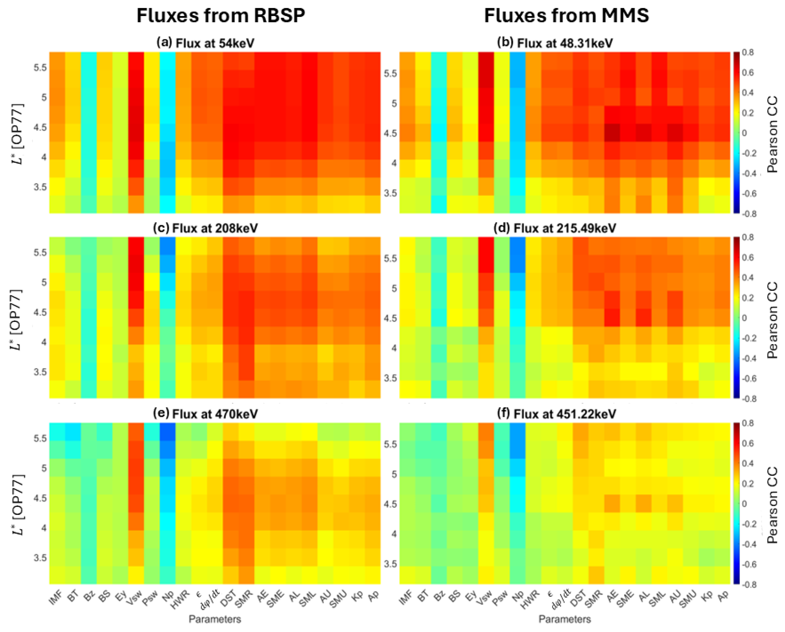
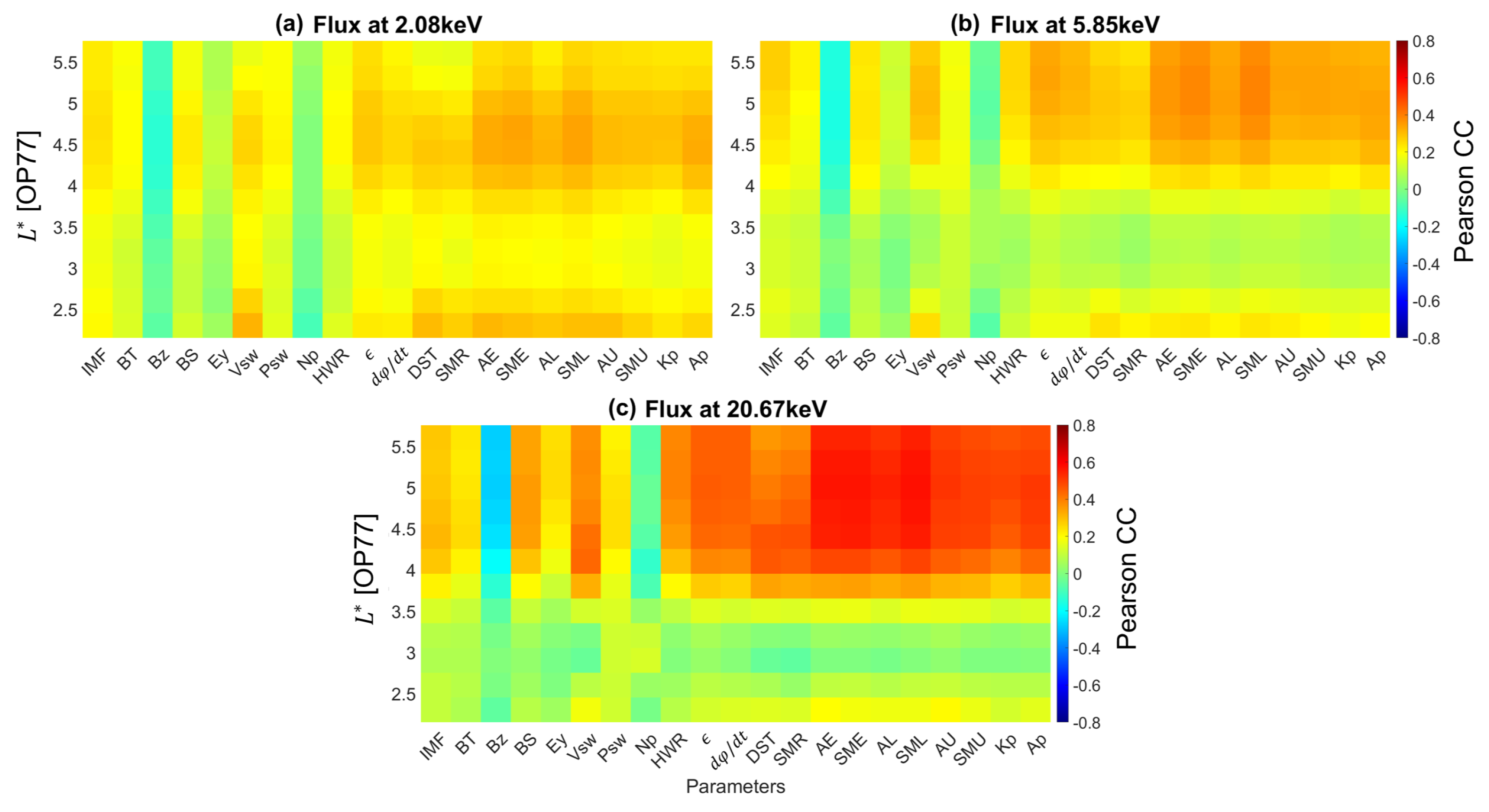
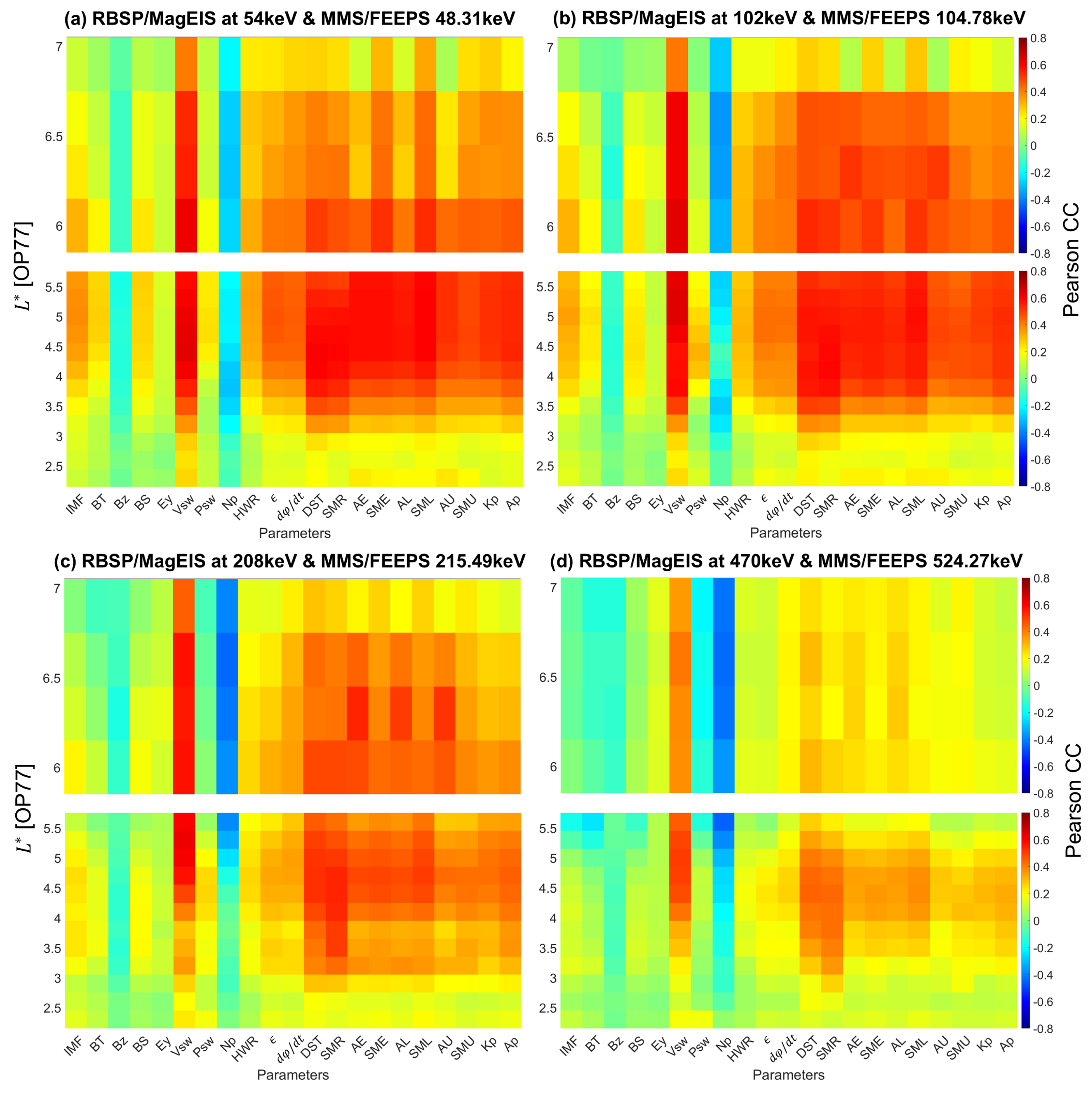
3.1. Results with Time Lag Set to Zero

Figure 2 shows the Pearson correlation coefficients between the various parameters and the electron differential flux as a function of $L^{*}$ (OP77) for the <50 keV electrons from RBSP. In general, the plots indicate that low-energy electron fluxes correlate with several important parameters, such as $V_{sw}$, the coupling functions, and most studied geomagnetic indices. The correlation between these parameters and energy flux < 10 keV is approximately 0.3 for $L^{*}>4$. Electrons with energies between 10 and 50 keV correlate better with these parameters, with coefficients reaching 0.7. Notably, as energy increases, strong correlation coefficients extend to progressively lower $L^{*}$ values. Additionally, for energies above 50 keV, the extended $L^{*}$ range of our analysis reveals that these fluxes correlate strongly with the parameters within a wide spatial range. However, the correlation coefficients of these parameters with the seed electron population (>100 keV) decrease significantly, except for $V_{sw}$, where the correlation remains consistently high. Moreover, for fluxes exceeding 300 keV, the correlation with the parameters is confined in a smaller $L^{*}$ range.

An individual examination of the parameters reveals that electron fluxes correlate strongly with the AE index over a wide energy range. Although the SME index behaves similarly, AE shows slightly higher correlation coefficients. The correlation of AL and SML with flux resembles that of AE and SME, respectively. Similarly, the Dst index shows comparable correlation patterns with the SMR index, although Dst generally has higher coefficients across energy channels. Moreover, the plots suggest that $V_{sw}$ is the most influential driver, with strongest correlation coefficients observed across most energy channels. Finally, both $B_z$ and $N_p$ show consistent negative coefficients, indicating an anti-correlation with the flux.

In more detail, starting with the lower energies (1–10 keV), electron fluxes demonstrate moderate correlation coefficients, around 0.25, mainly within the $L^{*}$ range [4–5], with the parameters IMF, $Bs$, and $V_{sw}$. The coupling functions and geomagnetic indices exhibit correlation coefficients at approximately 0.35 with the low-energy electron fluxes, while these coefficients also reach higher $L^{*}$ values (see Figure 2a). As energy increases within this range, strong correlation coefficients are exhibited toward higher $L^{*}$ values, particularly within the [4.25–6] range as shown in Figure 2b. Despite this shift, the correlation remains relatively constant at approximately 0.4. Notably, the correlation between these fluxes and the AE index is moderately strong, ranging from 0.3 to 0.45, representing the highest correlation observed across these energy channels. In contrast, the Dst and SMR indices show significantly lower correlation coefficients with this energy range, barely reaching 0.2. Similarly, the correlation between low-energy fluxes and $N_p$ is almost zero, while the coefficients for $B_z$ are approximately −0.2 within the $L^{*}$ range of [3.5–5].

At energies between 10 and 50 keV, the correlation coefficients between the various parameters and electron flux are stronger. The large coefficients are observed over progressively lower $L^{*}$ values, which offers us an insight into the spatial range occupied by each energy population. Specifically, in Figure 2c, strong correlation coefficients extend down to $L^{*}=3.75$. We observe that, as energy increases, the correlation of 10–25 keV electron fluxes with the AE index gradually strengthens, peaking at approximately 0.65. This behavior is also observed for the indices SME, AL, and SML. Additionally, in Figure 2c, the coefficients for Dst and SMR indices with the flux are around 0.35 for $L^{*}>3.75$, which is a notable increase compared to previous channels. On the other hand, the correlation of $N_p$ with the same population decreases to approximately −0.15 for $L^{*}>3.75$, while the correlation of $Bz$ reaches about −0.3 for $L^{*}>4.25$. A rapid change is observed in the correlation between $V_{sw}$ and electron flux. Previously limited to around 0.3 in lower-energy channels, the coefficients rise significantly for electrons with energies 10–50 keV. Specifically, as shown in Figure 2c, the correlation exceeds 0.5 across the $L^{*}$ range 3.75–6.

Figure 3 shows the Pearson correlation coefficients between the various parameters and the electron differential flux as a function of $L^{*}$ (OP77) for the >50 keV electrons from RBSP and MMS. Concerning the electrons with energies between 50 and 150 keV, the correlation coefficients between flux and solar wind/geomagnetic parameters increase significantly, reaching a peak of approximately 0.8 (see Figure 3a). Furthermore, these strong coefficients extend to lower $L^{*}$ values. Our extended analysis for energies above 50 keV, covering up to $L^{*}=7$, reveals that strong correlation coefficients also persist at higher $L^{*}$ values. To be precise, the coupling functions and geomagnetic indices are strongly correlated with energy fluxes in the 50–150 keV range across the $L^{*}$ interval [3.25–7], with coefficients around 0.6. The indices AE/SME and AL/SML are strongly correlated with the flux for $L^{*}$ values up to 7.5. The coefficients of these indices exceed 0.6 within the spatial interval $L^{*}$ = [4–6]. Additionally, the correlation of flux with the Dst and SMR indices increases, reaching values between 0.6 and 0.7. This is a significant improvement compared to lower-energy electrons, where the maximum correlation is approximately 0.3. Looking at the solar wind parameters, we observe that the correlation coefficients between $V_{sw}$ and the same electron population remain consistently high, at approximately 0.8, over a broader $L^{*}$ range of [3–7]. Moreover, the correlation of $N_p$ decreases across the entire $L^{*}$ range as energy rises, reflecting a stronger anti-correlation. The coefficients are also lower toward higher $L^{*}$ values. In particular, in Figure 3a, the coefficients are approximately −0.3 across the entire $L^{*}$ range, whereas, in Figure 3b, the values are below −0.5 for $L^{*}>6$. Notably, $B_z$ exhibits correlation coefficients around −0.15 with the flux for the entire $L^{*}$ range. IMF continues to correlate moderately with the electron flux, exhibiting correlation coefficients around 0.4 for $L^{*}$ = [3.75–6.25]. We also observe a weak correlation (coefficients hardly reaching 0.3) between the flux and $P_{sw}$ for $L^{*}$ = [4–5.25] in Figure 3b.

Fluxes of electrons with energies between 150 and 300 keV correlate strongly with the same parameters, though the coupling functions exhibit significantly lower coefficients compared to previous energy ranges. As shown in Figure 3c, the coupling functions display correlation coefficients around 0.3. Compared to lower-energy channels, the geomagnetic indices also exhibit slightly reduced correlations, with values around 0.5, and within a narrower spatial extent of $L^{*}$ = [3.75–6.75]. Among the geomagnetic indices, Dst and SMR exhibit the strongest correlation, extending down to $L^{*}=2.75$, which is lower compared to other parameters. Notably, the Dst index maintains large coefficients up to $L^{*}=7$, which is significantly higher than the spatial extent covered by other indices. Moreover, $V_{sw}$ continues to show the strongest correlation, with coefficients around 0.8 across a broad $L^{*}$ range of [2.5–7], which is the same spatial range as before. However, within the narrower $L^{*}$ = [2.5–4] region, the correlation decreases significantly, dropping to values near 0.3. Meanwhile, $N_p$ exhibits extremely low correlation coefficients with the flux, reflecting strong anti-correlation, reaching as low as −0.8 within $L^{*}$ = [5–8].

Lastly, the pseudocolor plots for energies between 300 and 500 keV reveal a significant decrease in the correlation coefficients between the flux and the geomagnetic indices, dropping to values around 0.3. These coefficients are also confined to a narrower spatial range of $L^{*}$ = [3.5–5.25], as shown in Figure 3d. Among the geomagnetic indices, Dst and SMR again show the strongest correlation with the flux (approximately 0.4), with the spatial extent reaching lower $L^{*}$ values compared to other parameters, specifically extending down to $L^{*}=2.75$. AE and AL show correlation coefficients around 0.3 within the $L^{*}$ = [3.5–5.25] and $L^{*}$ = [5.75–6.75] ranges. The correlation of $V_{sw}$ with the flux remains consistently high, exceeding 0.7 within the spatial range of $L^{*}$ = [3–7]. However, for $L^{*}>7$, the coefficients are approximately 0.4. $N_p$ exhibits trends similar to those observed in previous energy channels, with strong anti-correlation reaching −0.8 for $L^{*}$ = [5–7]. A notable difference is observed at lower $L^{*}$ values, where correlation was previously near zero, but now the coefficients are around −0.2. Lastly, a weak anti-correlation, with coefficients around −0.2, is observed between electron flux and $P_{sw}$ for $L^{*}>5.5$.

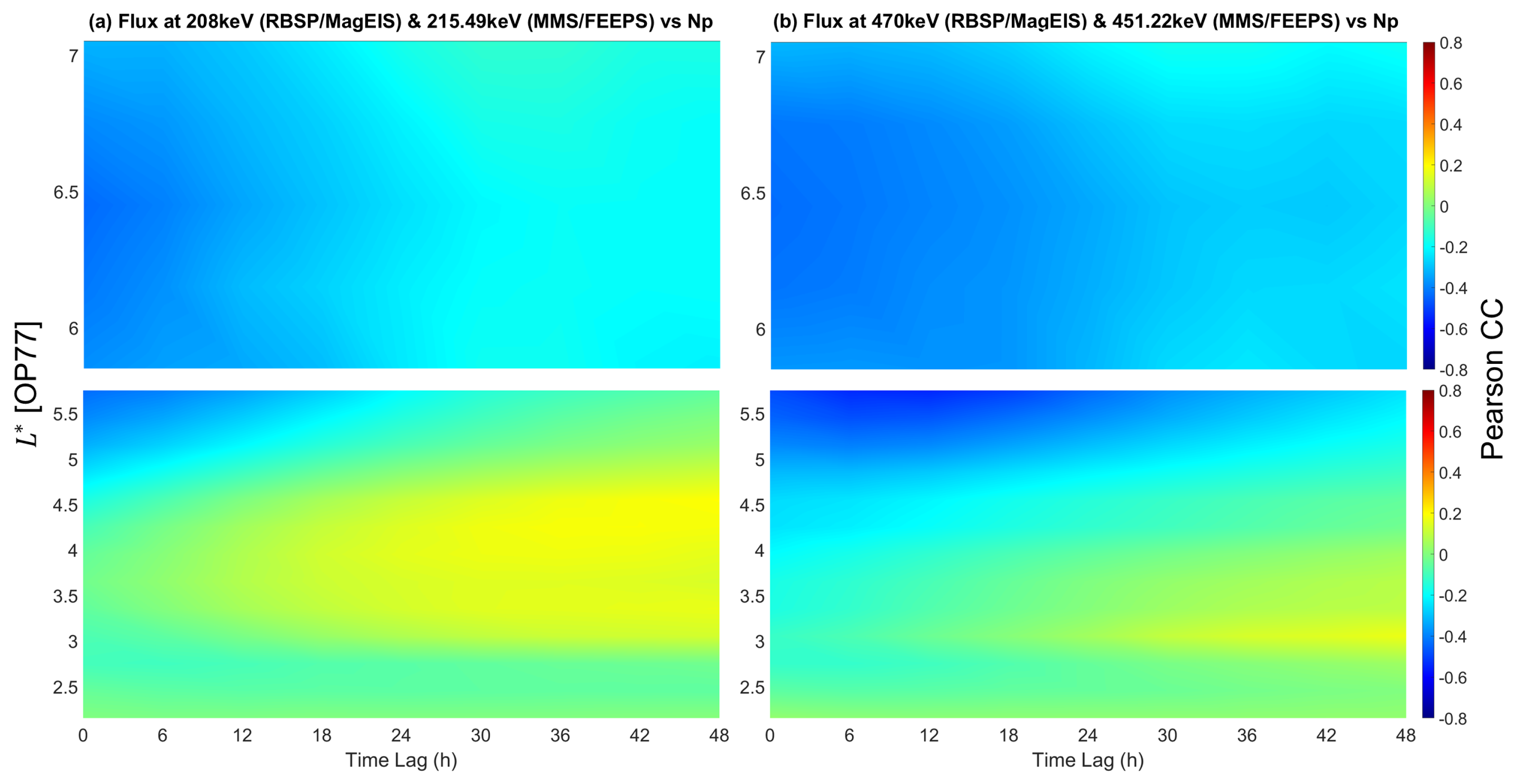
3.2. Results with Time Lag

As previously discussed, this analysis includes time lags to uncover the delayed responses of electron flux to changes in geospace conditions. To visualize these delays, pseudocolor plots are created, displaying time lags against $L^{*}$ for every parameter across all energy channels, with color corresponding to the correlation coefficients. The plots that we present belong to the third comparison of the analysis, which is the log(parameter)–log(flux). A high correlation is again defined as a correlation coefficient higher than 0.5, and lower than −0.5 for anti-correlations.

In prior analysis, we identified two parameters that exhibit stronger correlation and greater variability across energy channels. Specifically, we found that the solar wind velocity and the AE index are the most important drivers behind the sub-relativistic electron flux variations. To facilitate a more detailed examination of these parameters, we discuss the results of the correlation coefficients with respect to time lag.

3.2.1. Solar Wind Velocity

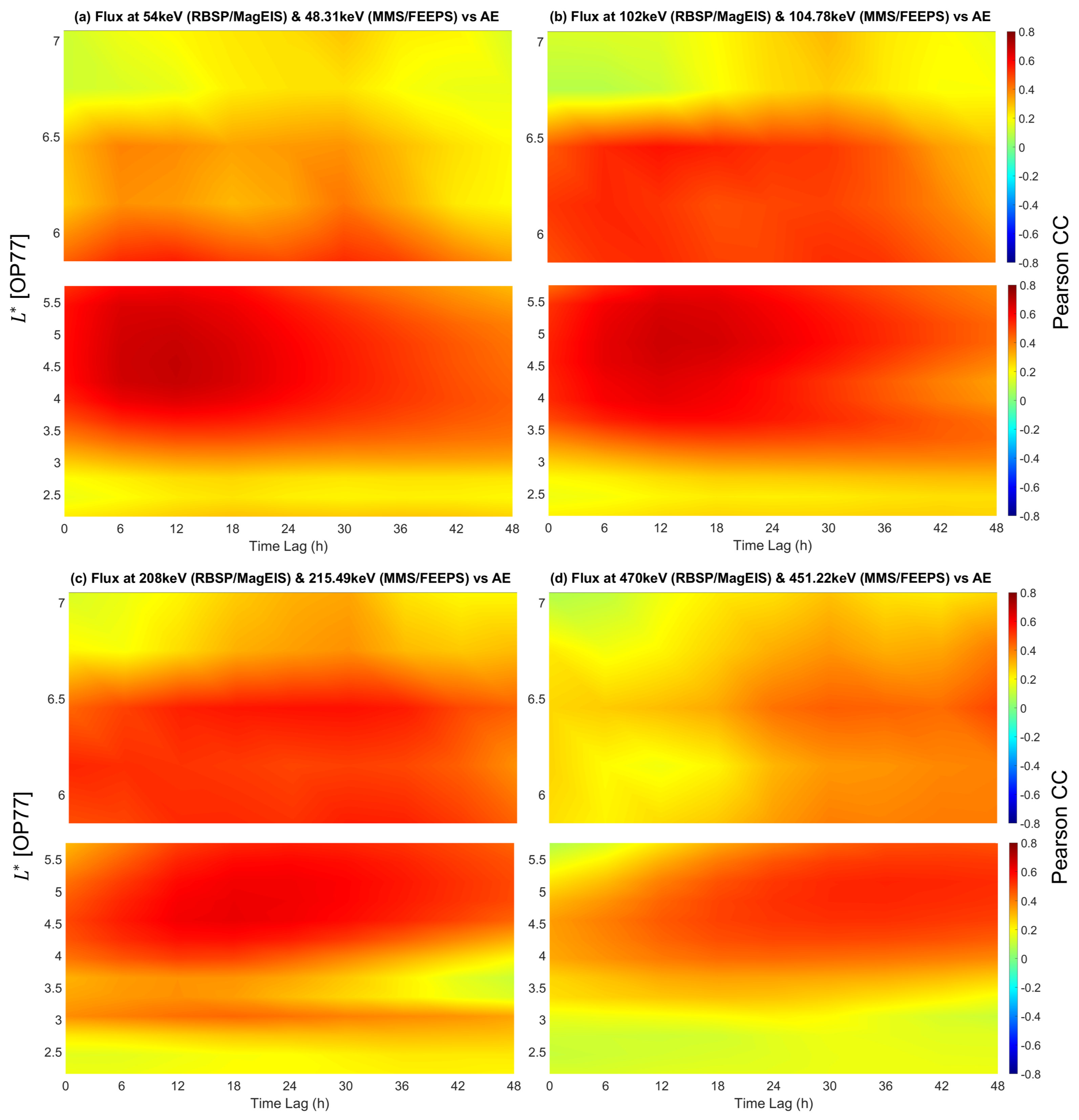
Among the plasma parameters, the solar wind velocity exhibits the most significant correlation coefficients with the electron flux. In particular, this parameter showed strong correlation with the seed electron population, where the coefficients reached a maximum value of 0.8. Notably, we observed some variability in the spatial extent of these correlation coefficients. Specifically, different energy channels revealed distinct $L^{*}$ regions where strong coefficients were observed.

Figure 4 shows the Pearson correlation coefficients between the parameter and the electron differential flux with a time lag as a function of $L^{*}$ (OP77) for the energy channels that we discuss. By incorporating time lags, we identify specific periods where the effects of the solar wind velocity are most pronounced. For low-energy electrons (<10 keV), the correlation remains low at short time lags. In contrast, electrons with energies above 10 keV exhibit higher correlation coefficients for time lags extending up to 48 h for certain energy channels.

As noted earlier, the low-energy electrons (<10 keV) exhibit a weak correlation with $V_{sw}$. For example, at 5.75 keV (see Figure 4a), the maximum coefficients, approximately 0.3, are observed for time lags of only 6 to 12 hours and are restricted to $L^{*}$ values above 4. As energy increases, electrons with energies between 10 and 50 keV correlate well with $V_{sw}$ for longer time lags. In Figure 4b, we observe that the correlation of flux with velocity is approximately 0.5 within the $L^{*}$ range of [3.5–4.5], lasting for 48 h. However, at higher $L^{*}$ values, these strong coefficients are confined to shorter time lags of 18 h. Furthermore, maximum coefficients, around 0.6, are also observed within the $L^{*}$ range of [3.5–4.5], but for time-lag values between 0 and 6 h.

For electrons with energies between 50 and 150 keV, correlation coefficients greater than 0.4 are observed throughout the entire time lag range for $L^{*}$ = [3–4]. However, for $L^{*}$ values in the range [4–6], strong coefficients are restricted to time lags of 0–24 h. Analysis of MMS fluxes further reveals that $V_{sw}$ is well correlated with this electron population across the entire time lag range within the $L^{*}$ range [6–7.6], with coefficients consistently above 0.4. In Figure 4c, the region showing the highest correlation has intensified, with coefficients reaching approximately 0.75. This peak is observed within the $L^{*}$ range [4–5.5], with time lags barely extending beyond 12 h. Furthermore, in Figure 4d, the correlation strengthens within the same $L^{*}$ and time lag ranges as before. However, the region where correlation peaks has shifted to higher $L^{*}$ values and now spans a wider spatial range of $L^{*}$ = [4.5–6.5], extending up to approximately 15 h.

For energies between 150 and 300 keV, the correlation of electron fluxes with $V_{sw}$ decreases significantly for $L^{*}<4$, except for a very narrow range at $L^{*}$ = [2.75–3.25], where the coefficients are around 0.4 for time lags of up to 30 hours. As shown in Figure 4e, within the spatial range of $L^{*}$ = [3.75–4.5], $V_{sw}$ exhibits correlation coefficients around 0.4 with the electron flux for progressively longer time lags, starting at 18 h and extending to approximately 30 h. For $L^{*}>4.5$, $V_{sw}$ maintains coefficients above 0.5 across the entire time range. The region where correlation peaks has shifted once again to higher $L^{*}$ values, now spanning $L^{*}=[5-6.5]$, within a time lag range of 6 to 18 h.

Lastly, for energies between 300 and 500 keV, $V_{sw}$ exhibits relatively constant correlation coefficients within the $L^{*}$ range [3–6], with no significant variation in the time lag values associated with strong coefficients. However, for $L^{*}>6$, the correlation decreases noticeably, with coefficients barely at 0.4 across the entire time lag rage. In Figure 4f, we observe that the region of peak correlation has shifted further along the x-axis, now spanning a time lag range of 18 to 36 h for $L^{*}$ = [5–6].

3.2.2. AE Index

Among the geomagnetic indices, the AE index consistently showed strong correlation with the flux across all energy channels, highlighting its role as a significant driver of flux variability in the radiation belts. By including time lags, the analysis reveals that the lower-energy channels exhibit moderate correlation coefficients, around 0.4, whereas higher-energy channels show much stronger correlations, with coefficients peaking at 0.8. Additionally, a notable variability is observed in the time lag and $L^{*}$ ranges associated with these high correlation coefficients, suggesting complex temporal and spatial dynamics.

Figure 5 shows the Pearson correlation coefficients between the parameter and the electron differential flux with a time lag as a function of $L^{*}$ (OP77) for the <50 keV electrons from RBSP. For low-energy electrons (<10 keV), we observe that the correlation with AE is moderate, with coefficients ranging between 0.3 and 0.4 for short time lags. For instance, as shown in Figure 5a, electrons at 2.08 keV correlate well with the index within the $L^{*}$ range [3.75–5.25], extending up to a time lag of 18 h. As energy increases within this range, this correlation strengthens. Electrons at 5.85 keV, as shown in Figure 5b, exhibit slightly larger coefficients, around 0.45, while the $L^{*}$ range significant correlation extends to 6. Moreover, the associated time lag increases, reaching over 24 h.

For energies between 10 and 50 keV, the correlation of flux with the index is significantly stronger, persisting over longer time lags compared to lower-energy channels. As shown in Figure 5c, correlation coefficients above 0.6 are observed within the $L^{*}$ range [3.5–4.5], lasting for up to 48 h. However, at $L^{*}$ values above 4.5, the correlation remains strong but is confined to shorter time lag values of 0–18 h.

Figure 6 shows the Pearson correlation coefficients between the parameter and the electron differential flux with a time lag as a function of $L^{*}$ (OP77) for the >50 keV electrons from RBSP and MMS. Starting from electrons with energies between 50 and 150 keV, we observe that the correlation with the AE strengthens notably, with coefficients peaking at 0.8 for certain time lag and $L^{*}$ values. This energy range demonstrates a sturdy dependence on geomagnetic activity (in terms of AE index), with strong correlation persisting across a broader spatial and temporal domain. Extended analysis covering up to $L^{*}=7.6$ reveals that strong correlation coefficients also persist at higher $L^{*}$ values. Specifically, in Figure 6a, correlation coefficients above 0.7 are observed consistently across the entire time lag range within the region $L^{*}$ = [3–6]. Beyond this, for $L^{*}$ = [6–6.8], strong correlation is evident, with coefficients around 0.6 for time lags of up to 36 h. A localized peak in correlation, reaching 0.8, is observed for $L^{*}$ = 4–6 within the time lag window of 5 to 20 h. As energy rises within this range, the correlation remains relatively stable. In Figure 6b, at $L^{*}$ values between 6 and 6.7, the correlation is increased and large coefficients are observed over longer time lags, reaching 48 h. The region of peak correlation shifts along the time lag axis, particularly to values between 6 and 24 h.

Electrons with energies in the range of 150 to 300 keV exhibit slightly weaker correlation coefficients with the AE index compared to lower energies. As shown in Figure 6c, below $L^{*}=3.75$, the correlation decreases significantly, with only a very narrow range at $L^{*}$ = [2.75–3.25] showing coefficients around 0.5. This localized correlation persists for time lags extending up to 48 h. However, for $L^{*}$ values in the range [3.75–6.7], the correlation is more robust, with coefficients consistently exceeding 0.65 across the entire time lag range. In this $L^{*}$ range, correlation is initially low, with coefficients hardly reaching 0.3 for the short time lag of 0 to 6 hours. As the time lag increases, the correlation coefficients strength. At $L^{*}$ = [7.1–7.5] and for time lags between 6 and 30 h, the index is correlate with the flux, showing coefficients around 0.65. The localized region of peak correlation, which reaches coefficients of nearly 0.7, is now more confined. Specifically, it occupies the spatial range of $L^{*}$ = 4.5–5.5 and has shifted to time lag values of 12 to 24 h.

Lastly, for electrons in the 300 to 500 keV energy range, the correlation between the index and flux weakens, while significant coefficients are associated with lower time lag and $L^{*}$ values. As shown in Figure 6d, at $L^{*}$ values between 3.5 and 6, AE exhibits coefficients around 0.5 for time lags above 6 h, lasting for 48 h. At higher $L^{*}$ values, the correlation becomes increasingly delayed, with coefficients around 0.4 appearing for time lags beyond 24 h.

4. Discussion

Using approximately 7 years of RBSP electron flux measurements and 9 years of MMS measurements, we have investigated in depth the influence of solar wind and geomagnetic parameters on the variability of 1–500 keV electrons in the inner magnetosphere by means of Pearson correlation analysis.

Alternative methods can provide deeper insights into the variability of the electrons. For instance, mutual information analysis measures the shared information of two variables and is a better measure of dependency for variables with a nonlinear relationship [28]. Wing et al. [29] demonstrated that conditional mutual information and transfer entropy can enhance modeling efforts by identifying the drivers of electron variability and also by detecting the changes in the dynamics. Moreover, Manshour et al. [30] applied conditional mutual information on fluxes of 54 keV to 2.23 MeV electrons and revealed that there is information transfer from solar wind and geomagnetic activity, as external drivers, into such fluxes. Although correlation analysis is the primary approach in this study, in future research, we aim to incorporate information theory methods to further explore causal dependencies and improve space weather modeling.

In general, our results indicate that, as energy increases, the correlation of flux with $V_{sw}$, the coupling functions, and most of the studied geomagnetic indices also increases. Low-energy channels (<10 keV) exhibit significant correlation coefficients with the parameters for $L^{*}>4$ but, as energy increases, strong correlation is observed over progressively lower $L^{*}$ values. This trend is consistent with high-energy electrons penetrating and getting trapped in lower L-shells [31].

We demonstrate that electron fluxes are best correlated with the solar wind velocity and AE index across most energy channels. This indicates that the variability of 1–500 keV electrons arises from a delicate interplay between mechanisms of which these parameters are proxies. Moreover, the results show that these mechanisms require progressively longer timescales to influence electron fluxes as energy increases. Li et al. [19], who studied GEO, observed that the time delay in the electron response to solar wind variations increases rapidly with energy. Therefore, our finding reveals that this trend is also evident at lower/higher $L^{*}$ values, i.e., inside and outside GEO.

Low-energy and source electrons, especially in the 20–100 keV range and at $L^{*}$ = [4–6], correlate well with the AE index, highlighting their direct link to substorm activity. However, seed electrons (>100 keV) exhibit weaker correlation with the AE index. This result is in agreement with Smirnov et al. [13]. Furthermore, Sillanpaa et al. [14] and Katsavrias et al. [12] reported similar behavior when they investigated the electron flux variability at GEO. The coupling functions and especially Newell’s function had comparable results and patterns with the AE index, although they exhibited lower correlation with the electron flux. This was expected, since Newell’s function is well correlated with the AE index [12,22]. The aforementioned result could be beneficial for modeling efforts, since Newell’s function is driven by solar wind parameters, which are provided in near-real time, in contrast with most geomagnetic indices.

The solar wind velocity $V_{sw}$, on the other hand, correlates well with electrons above 30 keV, while the highest correlation is exhibited with the seed population. This is in agreement with Katsavrias et al. [12], who showed that, as the energy increases (from the source to seed energy range), solar wind speed becomes a more important driver of electron flux at GEO.

The aforementioned behavior is expected at the heart of the outer radiation belt as well since low-energy and source electrons are primarily injected particles, mainly from substorms, whereas seed electrons arise from enhanced convection and/or inward radial diffusion [1]. Particularly, increased solar wind speed strengthens magnetospheric convection, enhancing the transport of electrons from the plasmasheet to the inner magnetosphere through substorm injections [32]. Moreover, high solar wind velocity enhances the Kelvin–Helmholtz instability at the magnetopause, generating ULF waves that can further accelerate the substorm-injected particles [33].

Regarding time delays in the response of electron flux, low-energy and source electrons (<100 keV) are strongly correlated with the AE index for the entire time lag range, which means that the electron flux is elevated for a period of 2 days after enhanced substorm activity. As energy increases, this correlation is associated with longer time lags, indicating a delay in the effect of substorm activity on electron fluxes. This delay is expected, as the region above $L^{*}=4$ is where chorus waves are generated through anisotropic distributions of source electrons, induced after intense substorms. Consequently, electrons could be interacting with VLF waves, leading to local acceleration (in situ heating) [34,35,36,37]. Since it takes longer for VLF waves to energize higher-energy electrons, this mechanism also explains the longer delays observed at higher energies.

Similarly, as energy increases, the correlation of solar wind velocity with the electron flux is observed over longer time lags. Specifically, the strong correlation of $V_{sw}$ with the seed population remains for up to 48 h. Previous studies have reported similar findings in terms of time lag only for relativistic electrons. Paulikas and Blake [17] had observed an increase in relativistic electron flux occurring 1–2 days after periods of elevated solar wind speed, a finding later confirmed by Horne et al. [38] and Reeves et al. [18]. The latter authors showed that the relationship between the electron fluxes and $V_{sw}$ is more complex than that suggested by previous statistical studies for both high and low energies at GEO.

Figure 7 presents a closer look at the variation in the maximum correlation coefficient as a function of $L^{*}$ and time lag. As shown, there is a very similar trend between the maximum correlation coefficients of ≈200 keV flux with solar wind speed and AE index. In detail, the maximum correlation coefficients associated with the AE index exhibit a consistently increased time lag by 12 h compared to the ones associated with solar wind speed. This may be another argument supporting the scenario that speed is the primary driver of seed electron enhancements and, furthermore, suggests that part of the population results from local acceleration processes. Nevertheless, the time delay of the response of seed electrons to solar wind speed is highly dependent on $L^{*}$. As shown, at $L^{*}$ = [3.5–4.5], the response of the seed electron flux due to solar wind speed variations is almost simultaneous. On the other hand, the response exhibits an increasing time delay as we move inward and outward from the heart of the outer belt, suggesting the further diffusion/transport of seed electrons. Moreover, the increase in the time delay below $L^{*}=3.5$ is much faster, suggesting that it takes a longer time for electrons to fill the slot region and the outer edge of the inner belt than to diffuse outward. Nevertheless, correlation coefficients below $L^{*}=3.5$ do not exceed the 0.5 threshold, probably due to the fact that very few solar wind speed enhancements can actually result in the filling of the slot region. Previous studies of Reeves et al. [39] and Katsavrias et al. [3] had shown that the impact of geomagnetic disturbances varies with electron energy and L-shells. The time delay presented in Figure 7 further supports this conclusion.

Finally, both $B_z$ and $N_p$ are anti-correlated with electron flux across the entire energy range that we study. Nevertheless, $B_z$ is weakly anti-correlated with all electron fluxes, whereas $N_p$ reveals strong anti-correlation with the seed electron population (100–500 keV). Above 200 keV, a significant anti-correlation is mainly observed for $L^{*}>4.5$, which gradually decreases at higher $L^{*}$ values. Moreover, as energy increases, the correlation decreases further (stronger anti-correlation). The parameter also shows stronger anti-correlation over longer time lags (Figure A5) and, at higher energies, the strong anti-correlations extends to lower $L^{*}$ values. The latter combination indicates the possibility of particle loss due to direct and/or indirect magnetopause shadowing, a term used for particles that are lost by drifting into the magnetopause. This means that higher-energy electrons, which have larger gyro-radii, are more susceptible to loss from lower L-shells [40,41].

Kellerman and Shprits [15] found that 31.7 keV electrons are correlated with density, while electrons with energies above 270 keV are anti-correlated with density. Our study yielded similar observations for seed electrons, but, for low-energy and source electrons, we found that $N_p$ exhibits low, yet important, anti-correlation with electron flux. A key factor that may explain the differing outcomes is the use of LANL-GEO geosynchronous satellites for the electron fluxes.

The coupling functions and especially Newell’s function had comparable results and patterns with the $AE$ index, although they exhibited lower correlations with the electron flux. This was expected, since Newell’s function is well correlated with the $AE$ index (Newell et al. [22]).The aforementioned conclusion could be very beneficial for future more accurate space weather prediction models.

5. Conclusions

Taking advantage of multimission measurements of electron fluxes in the outer radiation belt, we have investigated in depth the influence of solar wind parameters and geomagnetic indices on their variability. The results are summarized as follows:

• Electron fluxes are well correlated with $V_{sw}$ and the AE index across most energy channels, indicating that the variability of 1–500 keV electrons is the result of a delicate interplay between mechanisms for which these parameters are proxies. Additionally, these mechanisms require progressively longer timescales to influence electron fluxes as energy increases.
• Significant space weather parameters, i.e., $V_{sw}$, the coupling functions, and the geomagnetic indices, exhibit significant correlation with electrons at energies below 100 keV for $L^{*}>4$, with correlation coefficients increasing as energy rises. Furthermore, this strong correlation extends to lower $L^{*}$ values as the energy increases, suggesting broader spatial influence, possibly because higher-energy electrons penetrate and get trapped in lower L-shells more effectively than lower-energy electrons. However, the correlation between the seed electron population (100–500 keV) and the parameters decreases and is confined in a smaller $L^{*}$ range, except for $V_{sw}$, where correlation remains consistently high.
• $V_{sw}$ is one of the most influential driving parameters for fluxes above 50 keV. The correlation strengthens with increasing energy, and peaks for electrons in the 100–250 keV energy range, suggesting that solar wind speed plays a crucial role in the behavior of seed electrons. Electrons of energies higher than 200 keV correlate stronger with $V_{sw}$ after a lag of a few hours and until 48 h, indicating the importance of enhanced convection and/or radial diffusion.
• At the heart of the outer radiation belt, the response of the seed electron flux to solar wind speed variations is almost simultaneous, while the time lag values associated with the maximum correlation inwards and outwards of $L^{*}\approx$ 4 suggest further diffusion. Moreover, the rate that the time lag increases at the inward transport of electrons indicates that it takes longer for electrons to fill the slot region than to diffuse outwards.
• Electron fluxes correlate strongly with the AE index in a wide energy range, particularly for energies above 20 keV, highlighting the significant role of substorm activity in influencing the source and seed populations (local acceleration). Fluxes above 50 keV correlate well with AE across the entire time lag range. Seed electrons correlate stronger with the index after a few hours, suggesting a delay in the results of substorm activity on electron fluxes. This delay is also longer with increasing energy, starting from 5 h at 50 keV and reaching 1 day for energies above 200 keV.
• $N_p$ reveals strong anti-correlation with electron fluxes of energies 200–500 keV for $L^{*}>4.5$. With increasing energy, the correlation decreases further (stronger anti-correlation), indicating losses due to direct and/or indirect magnetopause shadowing.

Our results on the relationship between solar wind/geomagnetic parameters and the sub-relativistic electron flux in the inner magnetosphere, both in terms of correlation and the time delay of the response, can be beneficial for future modeling efforts via data-driven approaches.

References

1. Daglis, I.A.; Katsavrias, C.; Georgiou, M. From solar sneezing to killer electrons: Outer radiation belt response to solar eruptions. Philos. Trans. R. Soc. A 2019, 377, 20180097. [Google Scholar] [CrossRef]
2. Reeves, G.D.; McAdams, K.L.; Friedel, R.H.W.; O’Brien, T.P. Acceleration and loss of relativistic electrons during geomagnetic storms. Geophys. Res. Lett. 2003, 30, 1529. [Google Scholar] [CrossRef]
3. Katsavrias, C.; Daglis, I.A.; Li, W. On the statistics of acceleration and loss of relativistic electrons in the outer radiation belt: A superposed epoch analysis. J. Geophys. Res. Space Phys. 2019, 124, 2755–2768. [Google Scholar] [CrossRef]
4. Katsavrias, C.; Sandberg, I.; Li, W.; Podladchikova, O.; Daglis, I.A.; Papadimitriou, C.; Aminalragia-Giamini, S. Highly relativistic electron flux enhancement during the weak geomagnetic storm of April-May 2017. J. Geophys. Res. Space Phys. 2019, 124, 4402–4413. [Google Scholar] [CrossRef]
5. Li, W.; Thorne, R.M.; Ma, Q.; Ni, B.; Bortnik, J.; Baker, D.N.; Spence, H.E.; Reeves, G.; Kanekal, S.G.; Green, J.C.; et al. Radiation belt electron acceleration by chorus waves during the 17 March 2013 storm. J. Geophys. Res. Space Phys. 2014, 119, 4681–4693. [Google Scholar] [CrossRef]
6. Nasi, A.; Daglis, I.A.; Katsavrias, C.; Li, W. Interplay of source/seed electrons and wave-particle interactions in producing relativistic electron psd enhancements in the outer van allen belt. J. Atmos. Sol.-Terr. Phys. 2020, 210, 105405. [Google Scholar] [CrossRef]
7. Baker, D.N. The occurrence of operational anomalies in spacecraft and their relationship to space weather. IEEE Trans. Plasma Sci. 2000, 28, 2007–2016. [Google Scholar] [CrossRef]
8. Horne, R.B.; Glauert, S.A.; Meredith, N.P.; Boscher, D.; Maget, V.; Heynderickx, D.; Pitchford, D. Space weather impacts on satellites and forecasting the Earth’s electron radiation belts with SPACECAST. Space Weather 2013, 11, 169–186. [Google Scholar] [CrossRef]
9. O’Brien, T.P.; Lemon, C.L. Reanalysis of plasma measurements at geosynchronous orbit. Space Weather 2007, 5, S03007. [Google Scholar] [CrossRef]
10. Thomsen, M.F.; Henderson, M.G.; Jordanova, V.K. Statistical properties of the surface-charging environment at geosynchronous orbit. Space Weather 2013, 11, 237–244. [Google Scholar] [CrossRef]
11. Zheng, Y.; Ganushkina, N.Y.; Jiggens, P.; Jun, I.; Meier, M.; Minow, J.I.; O’Brien, T.P.; Pitchford, D.; Shprits, Y.; Tobiska, W.K.; et al. Space radiation and plasma effects on satellites and aviation: Quantities and metrics for tracking performance of space weather environment models. Space Weather 2019, 17, 1384–1403. [Google Scholar] [CrossRef] [PubMed]
12. Katsavrias, C.; Aminalragia–Giamini, S.; Papadimitriou, C.; Sandberg, I.; Jiggens, P.; Daglis, I.A.; Evans, H. On the interplanetary parameter schemes which drive the variability of the source/seed electron population at GEO. J. Geophys. Res. Space Phys. 2021, 126, e2020JA028939. [Google Scholar] [CrossRef]
13. Smirnov, A.G.; Kronberg, E.A.; Latallerie, F.; Daly, P.W.; Aseev, N.; Shprits, Y.Y.; Kellerman, A.; Kasahara, S.; Turner, D.; Taylor, M.G.G.T. Electron intensity measurements by the cluster/ RAPID/IES instrument in Earth’s radiation belts and ring current. Space Weather 2019, 17, 553–566. [Google Scholar] [CrossRef]
14. Sillanpää, I.; Ganushkina, N.Y.; Dubyagin, S.; Rodriguez, J.V. Electron fluxes at geostationary orbit from GOES MAGED data. Space Weather 2017, 15, 1602–1614. [Google Scholar] [CrossRef]
15. Kellerman, A.C.; Shprits, Y.Y. On the influence of solar wind conditions on the outer-electron radiation belt. J. Geophys. Res. Space Phys. 2012, 117, A05217. [Google Scholar] [CrossRef]
16. Shi, Y.; Zesta, E.; Lyons, L.R. Features of energetic particle radial profiles inferred from geosynchronous responses to solar wind dynamic pressure enhancements. Ann. Geophys. 2009, 27, 851–859. [Google Scholar] [CrossRef]
17. Paulikas, G.A.; Blake, J.B. Effects of the Solar Wind on Magnetospheric Dynamics: Energetic Electrons at the Synchronous Orbit. In Quantitative Modeling of Magnetospheric Processes; Geophysical Monograph Series; Olson, W.P., Ed.; American Geophysical Union: Washington, DC, USA, 1979; Volume 21, pp. 180–202. [Google Scholar] [CrossRef]
18. Reeves, G.D.; Morley, S.K.; Friedel, R.H.W.; Henderson, M.G.; Cayton, T.E.; Cunningham, G.; Blake, J.B.; Christensen, R.A.; Thomsen, D. On the relationship between relativistic electron flux, solar wind velocity: Paulikas and Blake revisited. J. Geophys. Res. Space Phys. 2011, 116, A02213. [Google Scholar] [CrossRef]
19. Li, X.; Baker, D.N.; Temerin, M.; Reeves, G.; Friedel, R.; Shen, C. Energetic electrons, 50 keV to 6 MeV, at geosynchronous orbit: Their responses to solar wind variations. Space Weather 2005, 3, S04001. [Google Scholar] [CrossRef]
20. Burton, R.K.; McPherron, R.L.; Russell, C.T. An empirical relationship between interplanetary conditions and Dst. J. Geophys. Res. Space Phys. 1975, 80, 4204–4214. [Google Scholar] [CrossRef]
21. Akasofu, S.-I. Energy coupling between the solar wind and the magnetosphere. Space Sci. Rev. 1981, 28, 121–190. [Google Scholar] [CrossRef]
22. Newell, P.T.; Sotirelis, T.; Liou, K.; Meng, C.-I.; Rich, F.J. A nearly universal solar wind-magnetosphere coupling function inferred from 10 magnetospheric state variables. J. Geophys. Res. Space Phys. 2007, 112, A01206. [Google Scholar] [CrossRef]
23. Burch, J.L.; Moore, T.E.; Torbert, R.B.; Giles, B.L. Magnetospheric Multiscale Overview and Science Objectives. Space Sci. Rev. 2015, 199, 5–21. [Google Scholar] [CrossRef]
24. Blake, J.B.; Mauk, B.H.; Baker, D.N.; Carranza, P.; Clemmons, J.H.; Craft, J.; Crain, W.R.; Crew, A.; Dotan, Y.; Fennell, J.F.; et al. The Fly’s Eye Energetic Particle Spectrometer (FEEPS) Sensors for the Magnetospheric Multiscale (MMS) Mission. Space Sci. Rev. 2016, 199, 309–329. [Google Scholar] [CrossRef]
25. Boyd, A.J.; Reeves, G.D.; Spence, H.E.; Funsten, H.O.; Larsen, B.A.; Skoug, R.M.; Blake, J.B.; Fennell, J.F.; Claudepierre, S.G.; Baker, D.N.; et al. RBSP-ECT Combined Spin-Averaged Electron Flux Data Product. J. Geophys. Res. Space Phys. 2019, 124, 9124–9136. [Google Scholar] [CrossRef] [PubMed]
26. Olson, W.P.; Pfitzer, K.A. Magnetospheric Magnetic Field Modeling. Annual Scientific Report. United States. 1977. Available online: https://www.osti.gov/biblio/7212748 (accessed on 4 December 2024).
27. Shue, J.-H.; Song, P.; Russell, C.T.; Steinberg, J.T.; Chao, J.K.; Zastenker, G.; Vaisberg, O.L.; Kokubun, S.; Singer, H.J.; Detman, T.R.; et al. Magnetopause location under extreme solar wind conditions. J. Geophys. Res. Space Phys. 1998, 103, 17691–17700. [Google Scholar] [CrossRef]
28. Johnson, J.R.; Wing, S. A solar cycle dependence of nonlinearity in magnetospheric activity. J. Geophys. Res. Space Phys. 2005, 110, A04211. [Google Scholar] [CrossRef]
29. Wing, S.; Johnson, J.R.; Camporeale, E.; Reeves, G.D. Information theoretical approach to discovering solar wind drivers of the outer radiation belt. J. Geophys. Res. Space Phys. 2016, 121, 9378–9399. [Google Scholar] [CrossRef]
30. Manshour, P.; Papadimitriou, C.; Balasis, G.; Paluš, M. Causal inference inthe outer radiation belt: Evidence for localacceleration. Geophys. Res. 2024, 51, e2023GL107166. [Google Scholar] [CrossRef]
31. Turner, D.L.; Fennell, J.F.; Blake, J.B.; Claudepierre, S.G.; Clemmons, J.H.; Jaynes, A.N.; Leonard, T.; Baker, D.N.; Cohen, I.J.; Gkioulidou, M.; et al. Multipoint Observations of Energetic Particle Injections and Substorm Activity During a Conjunction Between Magnetospheric Multiscale (MMS) and Van Allen Probes. J. Geophys. Res. Space Phys. 2017, 122, 11481–11504. [Google Scholar] [CrossRef]
32. Miyoshi, Y.; Kataoka, R.; Kasahara, Y.; Kumamoto, A.; Nagai, T.; Thomsen, M.F. High-speed solar wind with southward interplanetary magnetic field causes relativistic electron flux enhancement of the outer radiation belt via enhanced condition of whistler waves. Geophys. Res. Lett. 2013, 40, 4520–4525. [Google Scholar] [CrossRef]
33. Claudepierre, S.G.; Elkington, S.R.; Wiltberger, M. Solar wind driving of magnetospheric ULF waves: Pulsations driven by velocity shear at the magnetopause. J. Geophys. Res. Space Phys. 2008, 113, A05218. [Google Scholar] [CrossRef]
34. Shprits, Y.Y.; Subbotin, D.A.; Meredith, N.P.; Elkington, S.R. Review of modeling of losses and sources of relativistic electrons in the outer radiation belt II: Local acceleration and loss. J. Atmos. Sol.-Terr. Phys. 2008, 70, 1694–1713. [Google Scholar] [CrossRef]
35. Thorne, R.M.; Li, W.; Ni, B.; Ma, Q.; Bortnik, J.; Chen, L.; Baker, D.N.; Spence, H.E.; Reeves, G.D.; Henderson, M.G.; et al. Rapid local acceleration of relativistic radiation-belt electrons by magnetospheric chorus. Nature 2013, 504, 411–414. [Google Scholar] [CrossRef]
36. Bortnik, J.; Thorne, R.M.; Li, W.; Tao, X. Chorus waves in geospace and their influence on radiation belt dynamics. In Waves, Particles, and Storms in Geospace: A Complex Interplay; Balasis, G., Daglis, I.A., Mann, I.R., Eds.; Oxford University Press: Oxford, UK, 2016; pp. 193–212. ISBN 9780198705246. [Google Scholar]
37. Li, W.; Ma, Q.; Thorne, R.M.; Bortnik, J.; Zhang, X.J.; Li, J.; Baker, D.N.; Reeves, G.D.; Spence, H.E.; Kletzing, C.A.; et al. Radiation belt electron acceleration during the 17 March 2015 geomagnetic storm: Observations and simulations. J. Geophys. Res. Space Phys. 2016, 121, 5520–5536. [Google Scholar] [CrossRef]
38. Horne, R.B.; Thorne, R.M.; Glauert, S.A.; Meredith, N.P.; Pokhotelov, D.; Santolík, O. Electron acceleration in the Van Allen radiation belts by fast magnetosonic waves. Geophys. Res. Lett. 2007, 34, L17107. [Google Scholar] [CrossRef]
39. Reeves, G.D.; Friedel, R.H.; Larsen, B.A.; Skoug, R.M.; Funsten, H.O.; Claudepierre, S.G.; Fennell, J.F.; Turner, D.L.; Denton, M.H.; Spence, H.E.; et al. Energy-dependent dynamics of keV to MeV electrons in the inner zone, outer zone, and slot regions. J. Geophys. Res. Space Phys. 2016, 121, 397–412. [Google Scholar] [CrossRef]
40. Turner, D.L.; Shprits, Y.; Hartinger, M.; Angelopoulos, V. Explaining sudden losses of outer radiation belt electrons during geomagnetic storms. Nature 2012, 8, 208–212. [Google Scholar] [CrossRef]
41. Katsavrias, C.; Daglis, I.A.; Turner, D.L.; Sandberg, I.; Papadimitriou, C.; Georgiou, M.; Balasis, G. Nonstorm loss of relativistic electrons in the outer radiation belt. Geophys. Res. Lett. 2015, 42, 10521–10530. [Google Scholar] [CrossRef]
Figure 1. Comparison of the Pearson correlation coefficients between various parameters and the electron differential flux as a function of L * (OP77) for RBSP (left panels) and MMS (right panels). Pseudocolor plots show correlations for three energy channels: (top) RBSP 54 keV vs. MMS 48.31 keV, (middle) RBSP 208 keV vs. MMS 215.49 keV, and (bottom) RBSP 470 keV vs. MMS 451.22 keV.
Universe 11 00101 g001
Figure 2. Pseudocolor plots of the Pearson correlation coefficients between the parameters and the electron differential flux as a function of L * (OP77) for the following low-energy channels: (a) 2.08 keV, (b) 5.85 keV, (c) 20.67 keV.
Universe 11 00101 g002
Figure 3. Same as Figure 2 but for the following energy channels: (a) RBSP/MagEIS at 54 keV and MMS/FEEPS at 48.31 keV, (b) RBSP/MagEIS at 102 keV and MMS/FEEPS at 104.78 keV, (c) RBSP/MagEIS at 208 keV and MMS/FEEPS at 215.49 keV, (d) RBSP/MagEIS at 470 keV and MMS/FEEPS at 451.22 keV.
Universe 11 00101 g003
Figure 4. Pseudocolor plots of the Pearson correlation coefficients between V s w and the electron differential flux with time lag as a function of L * (OP77) for the following energy channels: (a) 5.85 keV, (b) 20.67 keV, (c) RBSP/MagEIS at 54 keV and MMS/FEEPS at 48.31 keV, (d) RBSP/MagEIS at 102 keV and MMS/FEEPS at 104.78 keV, (e) RBSP/MagEIS at 208 keV and MMS/FEEPS at 215.49 keV, (f) RBSP/MagEIS at 470 keV and MMS/FEEPS at 451.22 keV.
Universe 11 00101 g004
Figure 5. Pseudocolor plots of the Pearson correlation coefficients between the AE index and the electron differential flux with time lag as a function of L * (OP77) for the following energy channels: (a) 2.08 keV, (b) 5.85 keV, (c) 20.67 keV.
Universe 11 00101 g005
Figure 6. Same as Figure 5 but for the following energy channels: (a) RBSP/MagEIS at 54 keV and MMS/FEEPS at 48.31 keV, (b) RBSP/MagEIS at 102 keV and MMS/FEEPS at 104.78 keV, (c) RBSP/MagEIS at 208 keV and MMS/FEEPS at 215.49 keV, (d) RBSP/MagEIS at 470 keV and MMS/FEEPS at 451.22 keV.
Universe 11 00101 g006
Figure 7. Plot presenting the maximum time lag of correlation coefficients for 208 keV (RBSP/MAGEIS) and 215.49 keV (MMS/FEEPS) fluxes as a function of L * (OP77). Red circles and stars represent time lags corresponding to the solar wind speed ( V s w ) for RBSP and MMS, respectively. Blue circles and stars represent time lags corresponding to the AE index for RBSP and MMS. The dashed magenta line marks L * = 5.8 , the boundary between the data used from each mission. The x-axis shows time lag in hours.
Universe 11 00101 g007
Disclaimer/Publisher’s Note: The statements, opinions and data contained in all publications are solely those of the individual author(s) and contributor(s) and not of MDPI and/or the editor(s). MDPI and/or the editor(s) disclaim responsibility for any injury to people or property resulting from any ideas, methods, instructions or products referred to in the content.