Abstract
The beam exchange is a classical supplementary technique for spatio-temporal modulation in a dual-beam setup. In order to save time, the reduced polarimetric-optical-switching (RPOS) technique was propsed as an alternative technique. In this work, we revisit the assumptions of several formulas specifically constructed for this technique and evaluate their validity in different modulation schemes (e.g., dependent modulation), especially when reference measurements are acquired using specific Stokes signals. Subsequently, we compare the RPOS technique based on the most appropriate formula with the demodulation method based on the demodulation matrix by using synthesized observation data. The artificial observation takes into account the influence several factors have on the modulated intensities, including dark current, gain variation, atmospheric seeing fluctuations, and photon noise. Our numerical tests demonstrate that the RPOS technique has an advantage in mitigating the effects of atmospheric seeing fluctuations and gain variations between two beams. However, the selection of a specific Stokes signal for reference measurements has a notable impact on performance in minimizing the effect of photon noise.
1. Introduction
To analyze the polarization state (or full Stokes vectors) of incoming radiation, it is necessary to encode the Stokes vectors into intensity values that can be eventually registered by terminal detectors. This process is performed by an optical system called a polarimeter, which consists of a polarization modulator and an analyzer. In other words, the polarimeter is a combination of one or more retarders (as a modulator) followed by a polarizer or a polarizing beamsplitter (as an analyzer). At least four intensity measurements are required to retrieve the full Stokes vectors. This is achieved by changing the retardance or the relative orientation between the optical components. This mainly includes the temporal and spatial modulation schemes based on the different types needed to perform ([1], 1999). Each of them has different benefits in minimizing the effects of the two crucial factors on polarimetry precision, particularly for the ground-based observations, i.e., the gain table of the detectors and the atmospheric seeing. As reviewed by [2] (2019), by far the most widespread type of polarization modulation used in solar instruments is spatio-temporal modulation in the form of a dual-beam setup. In this setting, an adequate modulator changes its properties continuously or discretely over time, and a polarizing beamsplitter is used as a linear analyzer and is located after the temporal modulator splits the beam into two orthogonal polarization components (i.e., o and e components).
An alternative or supplementary technique to the spatio-temporal modulation, called beam exchange, was proposed by [3] (1990) based on the THEMIS polarimeter and was successfully applied to night astronomy (e.g., [3] 1990; [4] 1993) and solar observations ([5] 1998; [6] 2002). The beam exchange technique requires an extra measurement after exchanging the beams of two components, e.g., by using a rotating half-wave plate before the beamsplitter. The crucial step in the following demodulation involves constructing a specific formula to combine all the measurements of the two beams to retrieve the incoming with good approximation. Ref. [7] (2017) applied the beam exchange technique based on the FASOT-1 polarimeter for the 2013 solar total eclipse observation. They employed a liquid crystal variable retarder (LCVR), which is installed before the beam splitter, with its fast axis tilted at a 45-degree angle. One can quickly change its retardance from 0 to in a timescale of a few milliseconds by changing the voltage to perform the beam exchange.
In short, the greatest advantage of beam exchange is to overcome the uncertainty of intensity differences between two beams, which may arise from variations in detector gain or the transparency of optical components. A specific formula is constructed based on the ratio between two successive measurements (e.g., Equation (1) of [5] 1998). In this case, the flat-fielding process is theoretically unnecessary, and the accuracy is improved. However, it is a fact that this technique is inevitably time-consuming due to an extra measurement needed for each modulation step, which adversely affects the crucial assumption that the observed Stokes signal remains identical (with minimal variation) during the exchange. During one solar eclipse observation, ref. [7] (2017) used an alternative method to save time. They only performed the beam exchange measurement with a polaroid installed in front of the telescope after the eclipse observations (i.e., no beam exchange was performed during the eclipse observation). That is the reason they name it the reduced polarimetric optical switching (RPOS) technique (they rename the classical beam exchange as the polarimetric optical switching technique). It is worth noting that, in their work, only a single Stokes parameter was observed. They analyzed the signal-to-noise level in the demodulated profile and proposed a specific formula that is different from that of [3] (1990), while an alternative one was suggested in [8] (2022).
There are two facts: (1) either the THEMIS or the FASOT telescope is polarization-free, i.e., no polarization cross-talk is introduced by the instrument before the polarimeter; (2) both polarimeters adopt a modulation scheme that modulates Q, U, and V independently, i.e., , , and are obtained successively over time. However, in the present work, we pay more attention to the performance of the RPOS technique in other modulation schemes, with which the Stokes signals are not modulated independently. For example, one adopts a polarimeter based on a continuously rotating wave plate as a modulator. We are also interested in the performance of the RPOS technique when there is strong cross-talk introduced by the telescope before the polarimeter.
In Section 2, we simulate three types of modulation schemes for the full Zeeman-effect-induced Stokes parameters: one involves independent modulation, while the other two involve dependent schemes. We propose an alternative approach to beam exchange in order to conveniently obtain the so-called reference measurements in the RPOS technique. Using this approach, we re-check the validity of four formulas used by the RPOS technique and select the most appropriate one. In Section 3, the performance of the RPOS demodulation technique (with the correct formula) is compared with that using the demodulation matrix. This comparison takes into account the various factors influencing the observed intensities, including atmospheric seeing, dark current, gain variation of the detectors, and photon noise. The conclusion and discussion are presented in Section 4.
2. Observation Simulation
2.1. Modulation Schemes
The observation is simulated based on a polarimeter in a dual-beam setup, and the modulation schemes are determined by three types of temporal modulators, as shown below:
- (1)
- Scheme 1: The modulator consists of two quarter-wave plates, and both can individually rotate, e.g., the THEMIS polarimeter. Three measurements are taken by rotating two wave plates in the sequence of (0, 0), (0, 45), and (45, 0) during one modulation cycle with respect to the beam-splitter axis. In this scheme, the Stokes Q, U, and V are modulated independently and temporally. The outputs of the two beams need to be merged in the demodulation process.
- (2)
- Scheme 2: The modulator consists of one rotating half-wave plate and one fixed quarter-wave plate. Three measurements are sequentially taken at rotation positions of the half-wave plate (−90, −36, 18), while the position of the quarter-wave plate is fixed at 15 relative to the axis of the beam splitter. This scheme is employed by the FASOT polarimeter ([9] 2011; [10] 2023) to achieve high polarization modulation efficiencies over a wide wavelength range, using two commercial non-achromatic wave plates. In this way, the Stokes parameters are independently modulated, and merging the output of the two beams is also required for the demodulation.
- (3)
- Scheme 3: A continuously rotating wave plate with a certain retardance (e.g., 127) functions as a modulator. The rotation is performed at a certain frequency and synchronized observations are made by detectors. Typically, eight measurements are taken during one polarimetric cycle (a half rotation) successively, i.e., the wave plate undergoes a rotation of 22.5 during each exposure. It is adopted by, e.g., the Advanced Stokes Polarimeter (ASP; [11] 1992), the Solar Optical Telescope (SOT) polarimeter onboard Hinode (SP; [12] 2008), the spectropolarimeter on board the Aditya-L1 ([13] 2021). In this way, the Stokes parameters are also dependently modulated. However, in contrast to Scheme 2, it is unnecessary to combine the output of two beams for retrieving the full Stokes parameters. In other words, the polarimeter based on a one-beam setup can utilize this scheme, e.g., the New Vacuum Solar Telescope (NVST) polarimeter ([14] 2020).
In the first step, we ignore the polarization cross-talk before the polarimeter. Then, the modulated intensities in the i-th exposure for dual beams are given by,
here indicates the input Stokes signals to the polarimeter from the Sun. O is the theoretical modulation matrix (i.e., ). Except the elements in the first column, the other elements of and have equal magnitudes but opposite signs. indicates the rotation angle of the wave plate in the i-th exposure. In both Scheme 1 and Scheme 2, there are three exposures in each beam (i.e., ). In Scheme 3, with the sampling scheme of eight equally spaced intervals over a modulation period, there are eight times of exposure in each beam. (i.e., ). Taking the o beam as an example, Equation (1) can be written as
Supposing , we further have
Hereafter, the term , instead of , will be used in the following derivation.
2.2. Artificial Data
We make use of the RH code ([15] 2001) to synthesize the Zeeman effect-induced Stokes profiles . The synthesis is for the typical photospheric line Fe I 630.15 nm. By modifying the predetermined magnetic field strength and orientation, Stokes profiles of I, Q, U and V are generated as shown in Figure 1. The maxima of , , and are approximately , , and , respectively. Two detectors are assumed to operate synchronously in dual beams. A single row of pixels records the modulated intensity in the spectral dimension.
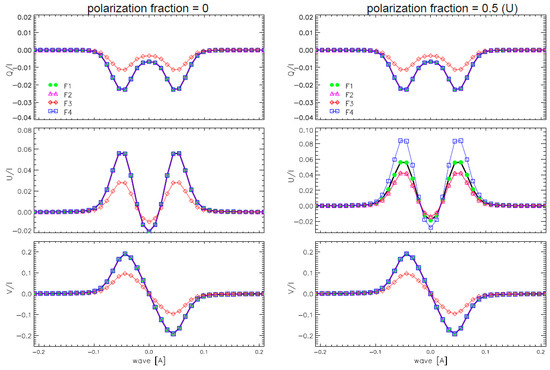
Figure 1.
Comparison of different formulas of the RPOS technique in the case of modulation Scheme 1. The black solid lines stand for the synthesized Stokes profiles, , , and , from top to bottom, respectively. The demodulated results obtained by different formulas are represented by the green dotted line (), pink triangular-shaped line (), red diamond-shaped line (), and blue square-shaped line (). (Left) using unpolarized for reference measurements. (Right) using partially polarized light with a fraction of .
Given several factors affecting the observations, the observed intensities at time t in the dual beams can be expressed as
We are reminded that a temporal modulation is performed at the time t (e.g., 3 or 8 measurements). g describes both the detector gain with pixel variation and the intensity imbalance between the two beams caused by the beam splitter. A variable s represents the temporal impact of seeing on each instant exposure, which varies slightly and randomly around 1 with a magnitude of at most a few percent. is the dark current of the detector and is assumed to remain constant along the wavelength without pixel variation. The photon noise, , in each pixel is signal-dependent and assumed to follow a Gaussian distribution with a standard deviation equal to the square root of the signal.
2.3. RPOS Technique: Formulas, Assumptions, and Applications
As suggested by the RPOS technique, two extra beam-exchange measurements are successively performed at out-of-observation times ( and ), which are referred to as reference measurements. The same applies to Equation (3); they are expressed as follows:
Next, two specific functions and are constructed to remove the influence of atmospheric seeing and gain g on . One can calculate the ratio between the two beams of each exposure, neglecting the dark bias () and photon noise ().
We need to note that here functions and are calculated for each measurement throughout the temporal modulations for both the scientific observations and the reference measurements.
Ref. [7] 2017 proposed four specific formulas () based on and to retrieve the Stokes signal under different assumptions, as summarized in Table 1 (it is important to note that in their work, X is equivalent to S since there is no modulator in their study). Inspired by his work on the acquisition of reference measurements, we propose an alternative approach to beam exchange: one can successively use a pair of specific input lights with opposite polarization states, e.g., input at time , and then input at to equally perform the beam exchange as described in Equation (4). In practice, it can be conveniently generated by using a specific optical component known as the instrument polarization calibration unit (ICU). It consists of a linear polarizer and a retarder. Both of them can rotate independently around the optical axis to generate well-defined Stokes vectors. The benefit of this approach lies in the stability of optics components, which ensures that the polarization fraction of the input signal remains constant, only with the sign reversing during the two successive measurements. But in contrast to the previous study, we consider different modulation schemes in this work, i.e., , which may lead to the assumptions of regarding no longer being valid. In the following, we analyze the validity of each formula for three types of schemes, especially using the alternative approach to obtain reference measurements.

Table 1.
The RPOS formulas and assumptions.
The main steps are modulating the synthesized data to generate the observed intensities (, ), then demodulating using to obtain , and finally calculating using . A comparison between the final result and the synthesized data is used to evaluate the validity of . Three types of modulation schemes are analyzed in the following.
- 1.
- For modulation Scheme 1, using specific polarized light (i.e., or or ) for reference measurements may result in the absence of intensity in one beam during temporal modulation, assuming dark current and photon noise are zero. For instance, if linearly polarized light with the polarization fraction equal to 1 is input at time , the function becomes invalid because equals 0 during one modulation step (note the reference axis to define the Stokes parameters is aligned with the beam-splitter axis, and is parallel to the polarization component in the o beam). The same problem occurs even if circularly polarized light is used. As a result, formulas are all meaningless. To address this issue, one potential resolution is to use unpolarized light, such as light from a quiet region on the solar disk ([16] 2005), as the target for the reference measurement. In this situation, as demonstrated in the left panel of Figure 1, the functions accurately fit the synthesized profile, but underestimates the signals. However, as the polarization fraction increases, the discrepancies caused by using become pronounced. For example, using with a polarization fraction for reference measurements leads to significant discrepancies in U retrieval, as shown in the right panel.
- 2.
- For Scheme 2, the issue in Scheme 1 is resolved by dependent modulation. However, as shown in Figure 2, using with a 100% fraction for reference measurements, only the formula can perfectly reproduce the synthesized profiles. The reason is straightforward: neither nor is negligible in this case, so the assumptions for other formulas are no longer valid. Furthermore, the validity of is not influenced by the polarization fraction of the input light. For instance, as shown in the right panel, when with a 10% fraction is used for reference measurements, the function can still work with high accuracy compared to the functions and , whereas the results from are still seriously underestimated.
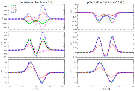 Figure 2. Same as Figure 1 but for the case of modulation Scheme 2: (Left) using for reference measurements; (Right) the polarization fraction is reduced to .
 - 3.
- For Scheme 3, from the comparisons in Figure 3, one can draw the same conclusion that formula is the only one to reproduce the synthesized Stokes profiles perfectly. In addition, this validity does not depend on whether linearly polarized light (left column) or circularly polarized light (right column) is used for reference measurements.
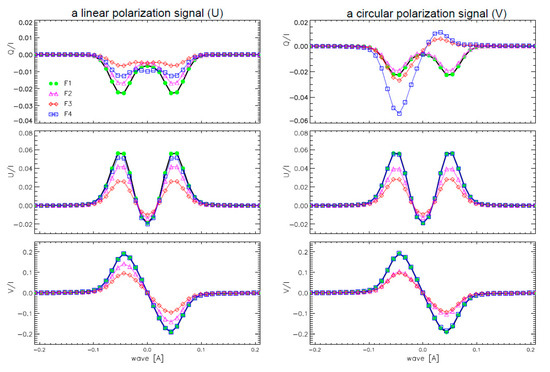 Figure 3. Same as Figure 1 but for the case of modulation Scheme 3: (Left) using for reference measurements; (Right) using .
In brief, if specific polarized light, i.e., , or , conveniently generated by an ICU, is utilized for reference measurements, and no changes in the polarization state are introduced before the modulator, the RPOS technique cannot be applied to Scheme 1. However, the RPOS technique can be applied to Schemes 2 and 3 only by performing formula . In addition, we admit that using unpolarized light for reference measurements is another potential method.
3. Comparison with Other Demodulation Methods
In this section, the demodulation based on formula (i.e., known as the RPOS technique) is compared with that based on the demodulation matrix (DM). In this case, the artificial observations take into account the impact of dark current, atmospheric seeing, detector gain, and photon noise.
Here, we adopt D to represent the optimum demodulation matrix given by the pseudo inverse of O as ([17] 2000). The polarization signal is derived by . It is worth noting the following: (1) For modulation Schemes 1 and 2, it is necessary to merge the outputs of o and e beams together for the demodulation, i.e., consists of and , and O is composed of and . (2) For the modulation Scheme 3, it is more favorable to demodulate each beam separately and then merge the results, i.e., , since each beam has its own dark current, gain table and throughput, etc. One can also use a specific operator to represent the demodulation procedure in each beam. For example, ref. [18] (1997) defined four operators with , where , = sign(cos4), = sign(sin4), = sign(−sin2). It is shown that these two methods are actually identical.
3.1. Effect of Dark Current
Dark current, including the stray light, is added to the intrinsic signal, so the dark current only affects the Stokes I profile, because the demodulation actually retrieves Stokes Q, U, and V by performing differences of measured intensities. As a result, the bias of Stokes I caused by the dark current will decrease the magnitude of retrieved Stokes , , and , and neither the RPOS technique nor DM has an advantage in this issue.
In order to minimize the Stokes I bias, one needs to have a good and accurate knowledge of the dark current. Most science requirements are met if the Stokes I level is known to about 1% ([19] 2013). In practice, the magnitude of stray light, as well as the spectral resolution, can be determined by comparing the fully reduced Stokes I profiles observed at disk center with a Fourier Transform Spectrum (FTS) obtained by [20] (1994).
3.2. Effect of Detector Gain Variation
In the case of modulation Scheme 3, either the o or e beam can be regarded as a single-beam configuration; the lack of knowledge about the gain variation of the detector can be overcome since all measurements are recorded by one detector. In other words, if there is no image displacement in these measurements, the flat-fielding is theoretically unnecessary to retrieve . In this section, therefore, our numerical test is only for Schemes 1 and 2, in which the gain variation treatment is essential.
We consider not only the pixel-to-pixel variations of each detector but also the different throughputs between the two beams (i.e., the imbalance between the two beam intensities): we assume that both detectors have a pixel-to-pixel variation with an amplitude of , which is approximately equal to the magnitude of . Additionally, we suppose there is an imbalance of in the throughputs between the two beams. As a result, for one detector, the gain factor is , and for the other detector, it is . The demodulated results are illustrated in Figure 4. It is seen that in Scheme 1 (left column), the retrieved Stokes profiles using the DM exhibit a zero-line offset (the blue line) compared to the input synthesized profile (the black line). This offset is attributed to the difference between and , and the pixel-to-pixel variation reduces the signal-to-noise ratio, making the profile almost indistinguishable. As mentioned in Section 2.3, the RPOS technique is not applicable in this scheme because we use specifically polarized signals for reference measurements. In Scheme 2 (right column), the performance of the RPOS technique (the green lines) demonstrates a significant advantage compared to the DM method, effectively mitigating these effects.
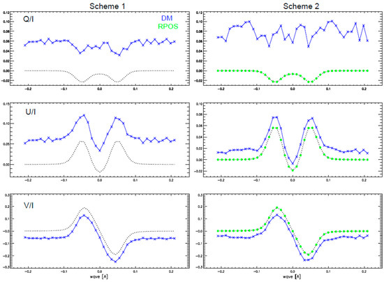
Figure 4.
Comparison of the influence of the gain variation. The cases of Scheme 1 and Scheme 2 are presented in the (left) and (right) columns, respectively. The black dotted lines represent the synthesized profiles. The green dotted lines represent the results by using the formula of the RPOS technique. The blue dotted lines represent the results of using the DM.
3.3. Effect of Atmospheric Seeing
The independent modulation scheme based on a dual-beam setup, such as Scheme 1, is well-known for its effective reduction of atmospheric turbulence, so in this section, we only consider Schemes 2 and 3, which account for atmospheric seeing effects with random intensity fluctuations of up to in each exposure.
Firstly, in both Schemes 2 and 3, unlike the impact of dark current, random intensity fluctuations result in an asymmetry discrepancy in all the retrieved Stokes profiles when using the DM method. As an example, we show the retrieval of in the upper-right panel of Figure 5 (see the blue and red profiles). This panel also displays the DM result of Scheme 3 using single-beam measurements (the pink profile), which also exhibits a zero-line offset proportional to the magnitude of the intensity fluctuation. This comparison further highlights the advantage of the two-beam configuration when intensity fluctuation is considered. However, when the RPOS technique is employed (in the lower-right panel), both the asymmetric discrepancy and the zero-line offset problems have been effectively addressed.
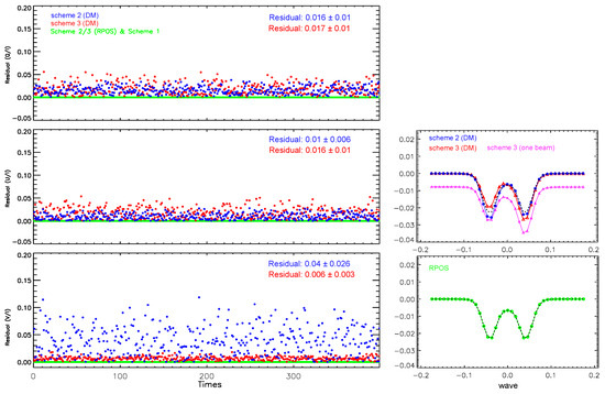
Figure 5.
Impact of random intensity fluctuations on the demodulated results: (Upper-right) The synthesized profile is plotted as a black dotted line; the DM result in Scheme 2 is represented by a blue dotted line, while that in Scheme 3 is shown in a red triangle line. The DM result using one-beam measurements from Scheme 3 is plotted as a pink triangle line. (Lower-right) The RPOS result is shown as a green dotted line, overlaid with the synthesized profile. (Left) The residuals of 400 trials. From top to bottom are the residuals of , , and , respectively.
Secondly, regarding the DM method only, we further compare its performance in Schemes 2 and 3 by calculating the residuals between the input synthesized () and the final retrieved () Stokes profiles. The residual is defined as
and the discrepancy is integrated across the wavelengths. We perform 400 trial attempts for both schemes, each with random intensity fluctuations of up to in each exposure. The statistical results are shown in the left panel of Figure 5. It is found that, despite Scheme 3 (red dots) involving eight exposures compared to the three in Scheme 2 (blue dots), the residuals in Scheme 3 are notably smaller, especially when the circular polarization signal is taken into account.
3.4. Effect of Photon Noise
In this section, we still focus on Schemes 2 and 3 since the RPOS technique is not applicable to Scheme 1. We assume that the photon noise in each pixel is signal-dependent and follows a Gaussian distribution with the standard deviation being the square root of the signal:
Additionally, we set , , and . We perform 400 trial attempts for both schemes and make a statistical analysis of the residuals.
Firstly, it is found that the residuals of the DM method are slightly smaller than those of the RPOS technique in both schemes. For example, in Scheme 3, the residual of the DM method is approximately 0.09 ± 0.011, whereas that of the RPOS method is around 0.12 ± 0.014 regardless of the specific polarized signal used for reference measurements. In Scheme 2, however, the issue becomes more complex as shown in the left panel of Figure 6: The residual of the DM method is about 0.14 ± 0.02 (the blue dots), while the residual of the RPOS technique varies depending on the polarization single used for reference measurements. Specifically, using for reference measurements (green dots) yields the smallest average demodulation residual for the three Stokes parameters (, , and from up to bottom), which are approximately , , and for , , and , respectively, while using for reference measurements (black dots) results in noticeable errors, especially in , reaching up to .
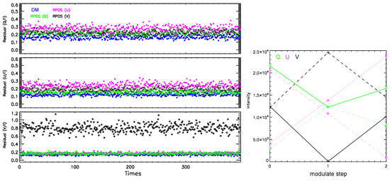
Figure 6.
Impact of photo noise on the demodulated results in Scheme 2: (Left) Statistics of residuals over 400 trials. Residuals of the DM method in blue (same as Figure 5) are compared with those of RPOS technique using different input polarization signals for reference measurements (green for , pink for and black for ). (Right) The modulated intensities of different input Stokes signals. Solid and dotted lines represent the intensity of the o and e beams, respectively.
In fact, the reason can be found in the modulation matrix of Scheme 2. The modulation matrix of the o beam can be written as
It is noted that the values of [2, 4] is nearly equal to −1, it means that, when the V signal is the input for reference measurements, the intensity of the o beam at the second modulation step is almost 0 (see the black solid line in Figure 6). Similarly, as [3, 3] = 0.925, the intensity at the third step becomes quite small when is the input (Note: the pink dashed line shows the case in e beam with U input, they are equal). In both cases, photon noise can seriously affect the modulated intensity. Therefore, we suggest that is the optimal choice for reference measurements in Scheme 2.
4. Discussion and Conclusions
Unlike the traditional beam-exchange technique, [7] proposed the RPOS technique, which performs the beam exchange outside the observation time using a specific polarization signal for reference measurements. Inspired by this work, we first propose an alternative approach for reference measurements, which successively inputs a pair of lights with opposite polarization states into the polarimeter instead of performing the beam exchange. This pair of input lights, i.e., Q and , U and , or V and signals, can be conveniently generated by a well-designed optical unit (e.g., an ICU) to ensure that only the polarization state, not the polarization degree (fraction), is changed in this process. In this context, we re-evaluate the applicability of four previously proposed formulas to other spatio-temporal modulation schemes in a two-beam setup, including those in the THEMIS, FASOT, and Hinode polarimeter (Schemes 1, 2, and 3). Our conclusions are as follows.
- 1.
- If specific polarized light is utilized for reference measurements, and no changes in the polarization state are introduced before the polarimeter (modulator), the RPOS technique is not suitable for Scheme 1. In this case, we suggest using unpolarized light, e.g., light from a quiet region near the solar disk center. In contrast, the RPOS technique can be applied to Scheme 2 and Scheme 3, but only by performing the formula ; other formulas are no longer valid. Furthermore, we find that the validity of is independent of the polarization fraction of the input signal. This implies that unpolarized light is also applicable in these scenarios.
- 2.
- If specific polarized light is utilized for reference measurements but significant cross-talk between the polarization states occurs due to the instruments in the polarimeter (modulator), the RPOS technique (with ) can be appropriate for these three schemes only if the cross-talk is stable during both the scientific and reference measurements. In this case, the cross-talk introduces a zero-line offset in the continuum of retrieved Stokes profiles.
- 3.
- A dual-beam setup offers the advantage of decreasing the effects of atmospheric seeing, while the RPOS technique further addresses issues related to detector gain variation and differences in throughput between the two beams, particularly compared with the DM method. However, when the effect of photon noise is considered, the performance of the RPOS technique is comparable to that of the DM method. Meanwhile, we note that for certain modulation schemes (e.g., Scheme 2), the selection of specific polarized signals used for reference measurements can influence the impact of photon noise.
In brief, for a traditional dual-beam polarimeter using a temporal modulation scheme, fluctuations of the intensity signal (e.g., atmospheric seeing) are encoded identically in two orthogonal polarization beams, so they can be eliminated from the operation via beam subtraction (i.e., the DM method). However, this design cannot effectively address the influence that arises due to a possible scaling factor between these two beams (e.g., the various gain and throughput). To address this issue, we propose to apply the RPOS technique, which, however, must be used with appropriate formulas and correct reference measurements. Furthermore, as large-aperture telescopes typically utilize ICU for instrumental polarization calibration, we propose using the ICU to facilitate the implementation of the RPOS technique.
Author Contributions
Methodology, Z.X.; software, Z.X.; validation, Z.X. and Y.Z.; formal analysis, Z.X. and Y.Z.; investigation, Z.X.; writing—original draft preparation, Z.X.; writing—review and editing, Z.X. and Y.Z.; funding acquisition, Z.X. All authors have read and agreed to the published version of the manuscript.
Funding
This research was funded by the National Science Foundation of China (NSFC) under the grant Nos. (12473054, 12127901, 12073075). The Strategic Priority Research Program of the Chinese Academy of Sciences grant No. XDB0560000. Yunnan Key Laboratory of Solar Physics and Space Science under the number 202205AG070009 and Yunnan Fundamental Research Projects under the numbers 202105AC160085.
Data Availability Statement
The synthesized data used for the numerical test are made by RH code, which is an open source, massively parallel radiative transfer code for spectral synthesis in stellar atmospheres. It is a modified version of the RH code by Han Uitenbroek. It is available in https://github.com/ita-solar/rh, accessed on 26 March 2023).
Conflicts of Interest
The authors declare no conflicts of interest. The funders had no role in the design of the study; in the collection, analyses, or interpretation of data; in the writing of the manuscript; or in the decision to publish the results.
References
- Collados, M. High Resolution Spectropolarimetry and Magnetography. In Proceedings of the Third Advances in Solar Physics Euro Conference: Magnetic Fields and Oscillations, Caputh, Germany, 22–25 September 1998; Schmieder, B., Hofmann, A., Staude, J., Eds.; Astronomical Society of the Pacific: San Francisco, CA, USA, 1999; Volume 184, pp. 3–22. [Google Scholar]
- Iglesias, F.A.; Feller, A. Instrumentation for solar spectropolarimetry: State of the art and prospects. Opt. Eng. 2019, 58, 082417. [Google Scholar]
- Donati, J.F.; Semel, M.; Rees, D.E.; Taylor, K.; Robinson, R.D. Detection of a magnetic region of HR 1099. Astron. Astrophys. 1990, 232, L1–L4. [Google Scholar]
- Semel, M.; Donati, J.F.; Rees, D.E. Zeeman-Doppler imaging of active stars. III. Instrumental and technical considerations. Astron. Astrophys. 1993, 278, 231–237. [Google Scholar]
- Bianda, M.; Stenflo, J.O.; Solanki, S.K. Hanle diagnostics of solar magnetic fields: The SR II 4078 Angstrom line. Astron. Astrophys. 1998, 337, 565–578. [Google Scholar]
- Bommier, V.; Molodij, G. Some THEMIS-MTR observations of the second solar spectrum (2000 campaign). Astron. Astrophys. 2002, 381, 241–252. [Google Scholar] [CrossRef][Green Version]
- Qu, Z.Q.; Dun, G.T.; Chang, L.; Murray, G.; Cheng, X.M.; Zhang, X.Y.; Deng, L.H. Spectro-Imaging Polarimetry of the Local Corona During Solar Eclipse. Sol. Phys. 2017, 292, 37–39. [Google Scholar] [CrossRef]
- Qu, Z.Q.; Chang, L.; Dun, G.T.; Xu, Z.; Cheng, X.M.; Deng, L.H.; Zhang, X.Y.; Jin, Y.H. Complexity of the Upper Solar Atmosphere Revealed from Spectropolarimetry during a Solar Eclipse. Astrophys. J. 2022, 940, 150–167. [Google Scholar]
- Qu, Z.Q. A Fiber Arrayed Solar Optical Telescope (FASOT). In Proceedings of the Solar Polarization 6, Maui, HI, USA, 30 May–4 June 2010; Kuhn, J.R., Harrington, D.M., Lin, H., Berdyugina, S.V., Trujillo-Bueno, J., Keil, S.L., Rimmele, T., Eds.; Astronomical Society of the Pacific: San Francisco, CA, USA, 2011; Volume 437, pp. 423–432. [Google Scholar]
- Wan, F.; Zhong, Y.; Qu, Z.; Xu, Z.; Zhang, H. Dual-beam polarimeter based on nonachromatic wave plates with high polarimetric efficiency over a broad band. Appl. Opt. 2023, 62, 2245–2255. [Google Scholar] [CrossRef] [PubMed]
- Elmore, D.F.; Lites, B.W.; Tomczyk, S.; Skumanich, A.P.; Dunn, R.B.; Schuenke, J.A.; Streander, K.V.; Leach, T.W.; Chambellan, C.W.; Hull, H.K. The Advanced Stokes Polarimeter—A new instrument for solar magnetic field research. In Proceedings of the SPIE Meeting, San Diego, CA, USA, 19–21 July 1992; Volume 1746, pp. 22–33. [Google Scholar]
- Ichimoto, K.; Lites, B.; Elmore, D.; Suematsu, Y.; Tsuneta, S.; Katsukawa, Y.; Shimizu, T.; Shine, R.; Tarbell, T.; Title, A.; et al. Polarization Calibration of the Solar Optical Telescope onboard Hinode. Sol. Phys. 2008, 249, 233–261. [Google Scholar] [CrossRef]
- Nagaraju, K.; Prasad, B.R.; Hegde, B.S.; Narra, S.V.; Utkarsha, D.; Kumar, A.; Singh, J.; Kumar, V. Spectropolarimeter on board the Aditya-L1: Polarization modulation and demodulation. Appl. Opt. 2021, 60, 8145–8153. [Google Scholar] [CrossRef] [PubMed]
- Hou, J.F.; Xu, Z.; Yuan, S.; Chen, Y.C.; Peng, J.G.; Wang, D.G.; Xu, J.; Deng, Y.Y.; Jin, Z.Y.; Ji, K.F.; et al. Spectro-polarimetric observations at the NVST: I. instrumental polarization calibration and primary measurements. Res. Astron. Astrophys. 2020, 20, 45–57. [Google Scholar] [CrossRef]
- Uitenbroek, H. Multilevel Radiative Transfer with Partial Frequency Redistribution. Astrophys. J. 2001, 557, 389–398. [Google Scholar]
- Stenflo, J.O. Polarization of the Sun’s continuous spectrum. Astron. Astrophys. 2005, 429, 713–730. [Google Scholar] [CrossRef]
- del Toro Iniesta, J.; Collados, M. Optimum modulation and demodulation matrices for solar polarimetry. Appl. Opt. 2000, 39, 1637–1642. [Google Scholar] [CrossRef] [PubMed]
- Skumanich, A.; Lites, B.W.; Martínez Pillet, V.; Seagraves, P. The Calibration of the Advanced Stokes Polarimeter. Astrophys. J. Suppl. Ser. 1997, 110, 357–380. [Google Scholar] [CrossRef]
- Lites, B.; Ichimoto, K. The SP_PREP Data Preparation Package for the Hinode Spectro-Polarimeter. Sol. Phys. 2013, 283, 601–629. [Google Scholar]
- Neckel, H. Solar Absolute Reference Spectrum. In Invited Papers from IAU Colloquium 143: The Sun as a Variable Star: Solar and Stellar Irradiance Variations; Pap, J.M., Frohlich, C., Hudson, H.S., Solanki, S.K., Eds.; Cambridge University Press: Cambridge, UK, 1994; pp. 37–44. [Google Scholar]


Disclaimer/Publisher’s Note: The statements, opinions and data contained in all publications are solely those of the individual author(s) and contributor(s) and not of MDPI and/or the editor(s). MDPI and/or the editor(s) disclaim responsibility for any injury to people or property resulting from any ideas, methods, instructions or products referred to in the content. |
© 2025 by the authors. Licensee MDPI, Basel, Switzerland. This article is an open access article distributed under the terms and conditions of the Creative Commons Attribution (CC BY) license (https://creativecommons.org/licenses/by/4.0/).