Inflection Point Dynamics of Minimally Coupled Tachyonic Scalar Fields

Abstract

In this paper, we explore the behavior of a minimally coupled tachyonic scalar field at an inflection point within an accelerating universe. We examine various cosmic expansion factors, including power-law, exponential, and a hybrid form combining power-law and exponential growth. For each of these scenarios, we derive the corresponding potentials of the tachyonic scalar field. Subsequently, we calculate the inflection points of the spatially homogeneous tachyonic scalar field for these potentials. To further analyze the system, we employ dynamical system analysis techniques to identify equilibrium points and assess their stability.

1. Introduction

Cosmic acceleration is now an established phenomenon. As supported by several cosmological and astrophysical observations [1,2,3,4,5,6,7,8,9,10] our universe is in a phase of accelerated expansion at the present stage. It is generally believed that, behind this accelerated expansion, there is a mysterious component, with negative pressure dominating $70\%$ of the universe. A promising candidate to explain this acceleration is “dark energy” [11,12,13,14,15], introduced as modified matter in Einstein’s field equations, that contributes to the energy–momentum tensor. One of the remarkable features of dark energy is its negative pressure and repulsive gravity characteristics led by the equation of state $w_{de}={\displaystyle \frac{p_{de}}{{\rho }_{de}}}$. On the other hand, there are also alternative gravity theories accounting for this cosmic acceleration by modifying the geometrical aspects of the field equation. Observational data from the Planck 2018 CMB [7,8,9,10] suggest that $70\%$ of the universe’s energy budget is in the form of dark energy, while the remaining $30\%$ of the energy budget of the universe is attributed to non-relativistic baryonic and non-baryonic pressureless ($p_m=0$) dust matter, with an equation of state (EoS) of $w_m=0$. In recent years, various candidates have been put forth to elucidate the nature of dark energy, with the cosmological constant standing out as one of the simplest models, embodying constant dark energy with an EoS of $w_{\Lambda }=-1$. Despite its alignment with observational data to a certain accuracy, the $\Lambda$ CDM model grapples with unresolved cosmological constant and coincidence problems [16,17,18,19,20]. In response to these limitations, dynamical dark energy models, particularly those involving scalar fields, have gained prominence [21,22,23,24,25,26], with scalar field serving as a candidate of dynamical dark energy; it is dubbed as $\varphi$ CDM and has a dynamical EoS $w_{\varphi }$. Recent data [27,28,29,30] also suggest a dynamical form of dark energy. The nature of dark energy has been the subject of several works in the literature. As alternatives to the cosmological constant, dynamic dark energy models have been developed, in which the EoS varies with time. There are many different dynamical dark energy models, such as quintessence fields [31,32,33], which possess tracker behaviour, and late time accelerating solutions of modified Friedmann equations lead by modification of gravity; other models include tachyon models, holographic dark energy models, chaplygin gas, phantom, k-essence, $\varphi CDM$, and $w\left(z\right)CDM$ [34,35,36,37,38,39,40,41,42,43,44,45,46,47].

Tachyonic scalar fields, originating from string theory, provide a compelling alternative to conventional scalar field dark energy models [48,49,50]. They represent the negative-mass mode within the open string perturbative spectrum; while their application in the dark energy domain is primarily phenomenological, we have specifically examined the behaviour of the scalar field near the inflection point. The study of scalar field dynamics in cosmology has been important in studying both early and late acceleration; moreover, in particular, a potential showing inflection can lead to an ultra slow-roll phase, sustaining the acceleration. Similar mechanisms arise in other contexts, such as the interplay between quantum and cosmological phenomena, where scalar fields play a significant role in bridging the gap between fundamental physics and large-scale cosmic evolution [51,52,53,54,55,56].

Recent studies by various researchers have also investigated dark energy models incorporating inflection points, particularly in the context of inflation [55,56,57,58,59,60,61,62,63,64,65,66,67,68,69,70,71,72,73,74], where the scalar field near an inflection point of the potential rolls slowly to produce inflation. Similarly, at low redshifts, an inflection point in the potential can cause the scalar field to roll slowly enough to explain cosmic acceleration. To study the dynamics and resulting behaviour of any scalar field model, the potential $V\left(\varphi \right)$ plays a pivotal role. A potential with an inflection point allows the field to exhibit a smooth transition (due to its flatness) between different cosmological phases by introducing a feature that facilitates slow rolling. When attempting to achieve a current equation of state value of $w_{\varphi }\approx -1$, which could lead to accelerated expansion, this slow-roll mechanism could be a key ingredient. By imposing the approximation in which the kinetic term ${\dot{\varphi }}^2$ of the tachyon is significantly smaller than unity, i.e., ${\dot{\varphi }}^2<<1$, we can position $\varphi$ in an extremely flat region of the potential. Potentials with an inflection point are good candidates for providing flat regions suitable for the ultra slow roll approximation. We consider the late-time behaviour of the tachyon scalar field in the accelerated expansion of the universe, which shares similarities with early inflation. Numerous authors have examined the cosmic behaviour of tachyonic scalar fields [49,75,76], discovering possibilities for both pure exponential growth and power-law expansion. We try to investigate the possibilities based on the superposition of these forms, because the current data have not yet determined the precise shape of the evolution of the scale factor.

Dynamical Setup

In this section, we present the mathematical framework on which the dynamics are based. We choose GR to be the background theory. The cosmological principle is encoded in the FLRW metric, which is expressed in terms of spherical co-moving coordinates, as follows:

$$d{s}^2=g_{\mu \nu }d{x}^{\mu }d{x}^{\nu }\equiv -d{t}^2+a^2\left(t\right)\left({\displaystyle \frac{d{r}^2}{1-K{r}^2}}+r^{2}d{\theta }^2+r^2{sin}^2\theta d{\varphi }^2\right).$$

(1)

Here, we have taken $c=1$. In the above equation, $a\left(t\right)$ is the scale factor and the parameter k is the spatial curvature, with the values $K=-1,0,1$ corresponding to spatially open, flat, and closed geometry, respectively. For our model, we have taken the effective four-dimensional action for the tachyonic field, which is given as follows [77,78]:

$$S_{\varphi }={\displaystyle \frac{1}{2{\kappa }^2}}\int d^{4}xf\left(\varphi \right)\sqrt{-g}R+\int d^{4}xV\left(\varphi \right)\sqrt{-g}\sqrt{\left(1+g^{\mu \nu }{\partial }_{\mu }\varphi {\partial }_{\nu }\varphi \right)},$$

(2)

where $V\left(\varphi \right)$ represents the potential, ${\kappa }^2={\displaystyle \frac{1}{M_p^2}}=1$, and $f\left(\varphi \right)=1$ under minimal coupling. This action introduces a non-canonical scalar field with a modified (DBI) kinetic term, often inspired by high-energy theories. The square-root structure resembles the DBI action from string theory. The energy–momentum tensor for Equation (2) can be written as follows:

$$T_{\mu \nu }^{\left(\varphi \right)}={\displaystyle \frac{V\left(\varphi \right){\partial }_{\mu }\varphi {\partial }_{\nu }\varphi }{\sqrt{1+g^{\alpha \beta }{\partial }_{\alpha }\varphi {\partial }_{\beta }\varphi }}}-g_{\mu \nu }V\left(\varphi \right)\sqrt{1+g^{\alpha \beta }{\partial }_{\alpha }\varphi {\partial }_{\beta }\varphi }$$

(3)

Einstein’s field equation for a spatially flat universe ($K=0$) gives the Friedmann equations as follows:

$$H^2={\left({\displaystyle \frac{\dot{a}}{a}}\right)}^2={\displaystyle \frac{8\pi G}{3}}\rho ,$$

(4)

and

$${\displaystyle \frac{\ddot{a}}{a}}=-{\displaystyle \frac{4\pi G}{3}}(\rho +3p),$$

(5)

where $H\left(t\right)\equiv {\displaystyle \frac{da}{dt}}$ is the Hubble parameter and $\rho ={\rho }_{\varphi }+{\rho }_m$ and $p=p_{\varphi }+p_m$ denote the total energy and the pressure, respectively. In general, multiple components, such as matter, radiation, and dark energy, can contribute to the energy–momentum tensor, each with a different equation of state. However, during early time periods, radiation dominated, after which matter started dominating more effectively. At later time periods ($z⟶0$), dark energy dominated the universe, leading to cosmic acceleration. We are therefore driven to focus on only two components: pressureless matter and dark energy. For cosmic acceleration, we have $\rho +3p<0$. The continuity equation is given as follows:

$$\dot{\rho }+3H(1+w)\rho =0.$$

(6)

where

$${\rho }_{=}{\rho }_m+{\rho }_{\varphi }$$

(7a)

and

$$p_{=}{p}_m+p_{\varphi }$$

(7b)

In Section 2, the investigation of the behaviour of the tachyonic scalar field is carried out near the inflection point. We consider three different possibilities of cosmic behaviours; the first two cases involve conventional power-law expansion and pure exponential growth, i.e., $a\left(t\right)=\alpha t^n,a\left(t\right)=\gamma e^{\beta t}$, respectively, and the third case is of quasi-exponential expansion of the scale factor $a\left(t\right)=\eta t^n{e}^{\beta t}$. For these three cases, we calculate the respective potentials and then investigate the behaviour of that particular model near their respective inflection points. In Section 3, dynamical analysis for the above two cases is carried out.

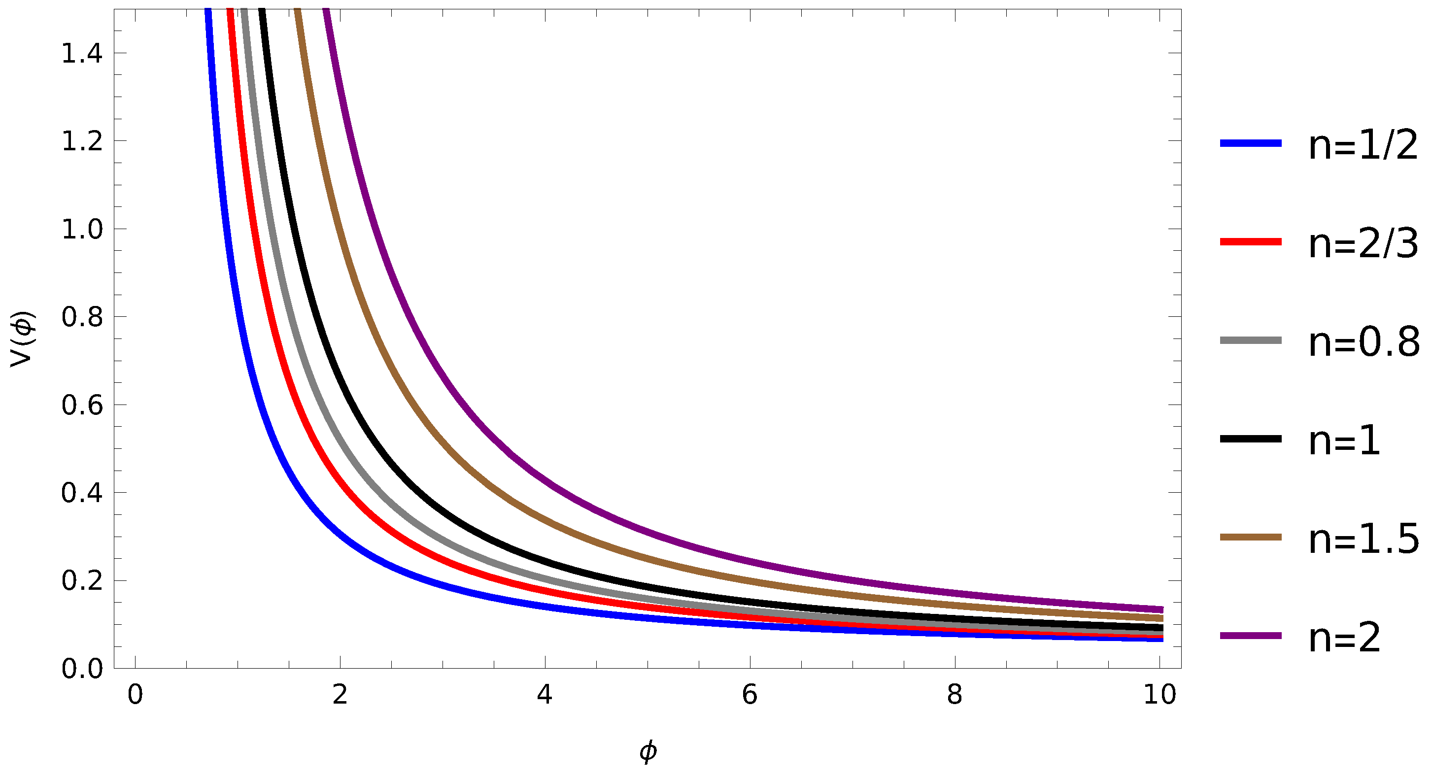
2. Inflection Point of Tachyonic Scalar Field

Using Equation (3) for a flat ($K=0$) FRLW universe, the energy density and pressure for the tachyonic scalar field are given as follows:

$${\rho }_{\varphi }={\displaystyle \frac{V\left(\varphi \right)}{\sqrt{1-{\dot{\varphi }}^2}}},$$

(8)

$$p_{\varphi }=-V\left(\varphi \right)\sqrt{1-{\dot{\varphi }}^2}.$$

(9)

Here, the overdot denotes the derivative with respect to time. $V\left(\varphi \right)$ is the potential associated with the tachyonic field that we have calculated in the upcoming subsections for each case.

By using the following equation:

$${\displaystyle \frac{\ddot{a}}{a}}=H^2+\dot{H}$$

(10)

and plugging Equations (8) and (9) into Equations (4) and (5) for the scalar field, we obtain the following form of the second Friedmann equation:

$${\displaystyle \frac{\ddot{a}}{a}}={\displaystyle \frac{{\kappa }^{2}V\left(\varphi \right)}{3\sqrt{1-{\dot{\varphi }}^2}}}\left(1-{\displaystyle \frac{3}{2}}{\dot{\varphi }}^2\right)$$

(11)

Now, for the accelerated expansion of the universe, we have $\ddot{a}>0$; thus, using Equation (11) and ${\dot{\varphi }}^2<{\displaystyle \frac{2}{3}}$, the EoS (equation of state) for $\varphi$ is given by the following equation:

$$w_{\varphi }={\displaystyle \frac{p_{\varphi }}{{\rho }_{\varphi }}}=({\dot{\varphi }}^2-1)$$

(12)

In terms of Hubble parameter, the equation of state $w_{\varphi }$ can be written as follows:

$$w_{\varphi }=-1-{\displaystyle \frac{2\dot{H}}{3H^2}}$$

(13)

For cosmic acceleration, the possible range of the values of $w_{\varphi }$ is $-1\le w_{\varphi }<-{\displaystyle \frac{1}{3}}$ and $0<{\dot{\varphi }}^2<{\displaystyle \frac{2}{3}}$. Using Equations (8) and (9), one can easily find the equation of motion for this tachyonic model, as follows:

$${\displaystyle \frac{\ddot{\varphi }}{(1-{\dot{\varphi }}^2)}}+3H\dot{\varphi }+{\displaystyle \frac{1}{V}}{\displaystyle \frac{dV}{d\varphi }}=0.$$

(14)

Now, using Equations (4) and (5), $\varphi \left(t\right)$ and $V\left(\varphi \right)$ can easily be written in the forms of H and $\dot{H}$, as follows:

$$\varphi \left(t\right)=\int \left(dt\sqrt{-{\displaystyle \frac{2\dot{H}}{3H^2}}}\right)$$

(15)

$$V\left(t\right)={\displaystyle \frac{3H^2}{{\kappa }^2}}\sqrt{1+{\displaystyle \frac{2\dot{H}}{3H^2}}}$$

(16)

Using the two equations above, we are able to find the potential and their respective inflection point behaviour for the three cases discussed below.

2.1. For Case I: $a\left(t\right)=\alpha t^n$

In this subsection, we consider the simplest model for describing the expansion of the universe in certain cosmological scenarios, namely, the power-law form of scale factor; this suggests that the universe’s expansion follows a simple power-law relationship with time. i.e., $a\left(t\right)=\alpha t^n$. Here, $\alpha$ is a constant describing the overall scale of the universe, and the exponent n determines the rate of expansion—it has to be greater than 0 for the universe to experience accelerated expansion. For this kind of model, the Hubble parameter is in the following form:

$$H={\displaystyle \frac{n}{t}}$$

(17)

Upon substituting this value of H into Equation (16) and using Equation (15), we obtained the following form of the potential:

$$V\left(\varphi \right)=V_0{(\varphi -{\varphi }_0)}^{-2}$$

(18)

where $V_0={\displaystyle \frac{2n}{{\kappa }^2}}\sqrt{1-{\displaystyle \frac{2}{3n}}}$. From the above Equation (18), we found there is no such inflection point for this particular model; we can also see in Figure 1 that the curve shows no inflection, but one can observe that the scalar field is rolling slowly along the potential. One can apply slow roll approximation directly into Equation (14) using ${\dot{\varphi }}^2<<1\Rightarrow 1-{\dot{\varphi }}^2\approx 1$ and can find the evolution of the scalar field with respect to time, but, in this case, $w_{\varphi }$ will be very close to $-1$. However, in our case, we have calculated the evolution equation directly from Equation (15), resulting in the following equation:

$$\varphi \left(t\right)=\sqrt{{\displaystyle \frac{2}{3n}}(t^2-t_0^2)}+{\varphi }_0$$

(19)

where $t=t_0$ when $\varphi ={\varphi }_0$, and the equation of state (Equation (13)) is as follows:

$$w_{\varphi }=-1+{\displaystyle \frac{2}{3n}}$$

(20)

For $n=2/3$, the scale factor evolves as $a\propto t^{2/3}$, corresponding to a matter-dominated universe, and as we can see from Figure 1 the potential corresponding to this case vanishes. This, in return, leads to $p_{\varphi }=0$, which corresponds to pressureless fluid with $w_{\varphi }=0$. For $n>2/3$, the equation of state satisfies $w_{\varphi }>-1$, indicating a quintessence-like behaviour. If we set $n>1$, then the equation of state satisfies $w_{\varphi }<-1/3$, which is a necessary condition for late-time cosmic acceleration. This supports an expanding universe consistent with observations of dark energy-driven acceleration.

In terms of cosmological redshift, we can also rewrite the above Equation (19) as follows:

$$\varphi (1+z)=\sqrt{{\displaystyle \frac{2}{3n{\alpha }^{2/n}}}}\sqrt{\left({\left({\displaystyle \frac{1}{1+z}}\right)}^{2/n}-{\left({\displaystyle \frac{1}{1+z_0}}\right)}^{2/n}\right)}+{\varphi }_0$$

(21)

Here, the initial value of redshift is taken to be $z_0⟶1100$. Figure 2 shows the evolution of $\varphi$ for different values of n. Also, $\alpha$ is a normalization constant and, for simplicity, is taken to be unity. We examine the behaviour of a scalar field $\varphi$ with respect to redshift z. As the redshift z approaches zero, $\varphi \left(z\right)$ increases asymptotically with $z⟶0$, corresponding to the late-stage evolution of the universe. The field is characterized by a unique potential which is derived from the scale factor; this potential governs its dynamics and the corresponding impact on cosmic expansion. Here, the case $n<1$ is of interest, as it provides a smooth/slow evolution of the scalar field $\varphi$ at a late epoch, resulting accelerated expansion at a late stage. This slow-roll regime results in the field behaving similarly to a cosmological constant, with a near-constant energy density. As a consequence, the universe continues to expand at an accelerating pace.

2.2. For Case II: $a\left(t\right)=\gamma e^{\beta t}$

For this particular case, we take the simplest exponential form of the scale factor $a\left(t\right)=\gamma e^{\beta t}$, where $\gamma$ and $\beta$ are the constants. $\beta$ determines the overall rate at which the scale factor changes and can have two possibilities for its values, as follows: the first possibility is $\beta >0$, which implies the exponential growth of the universe, i.e., an expanding universe; the second possibility is $\beta <0$, which implies exponential decay, i.e., a contracting universe. As we know, during early epochs the universe experienced expansion, so we can discard the second possibility. Now, the second constant $\gamma$ is a normalization factor that sets the overall scale of the universe at a particular time t, and H for this exponentially expanding universe is proportional to the constant below:

$$H=\beta$$

(22)

Now, using this value of H in Equations (15) and (16), we obtain the following form of potential:

$$V\left(\varphi \right)={\displaystyle \frac{3{\beta }^2}{{\kappa }^2}}$$

(23)

Therefore, for this particular model, there is no inflection point because the potential is revealed to be constant; this is consistent with the quintessence model, if the same calculations are carried out for the quintessence model with the same scale factor. Using Equations (14) and (23) and after applying the slow roll approximation, the scalar field $\varphi$ is also revealed to be a constant.

2.3. For Case III: $a\left(t\right)=\eta t^n{e}^{\beta t}$

For this case, we consider the universe to be the mixed form of the scale factor given by $a\left(t\right)=\eta t^n{e}^{\beta t}$, i.e., the product of power-law and exponential terms, where $\eta$, n and $\beta$ are the constants determining the overall rate at which the scale factor changes. For this model, the Hubble parameter is obtained as follows:

$$H={\displaystyle \frac{n}{t}}+\beta$$

(24)

Using Equations (15), (16), and (24), we can derive the following form of potential and the scalar field, in terms of t, as follows:

$$V\left(t\right)={\displaystyle \frac{3{(n+\beta t)}^2}{{\kappa }^2{t}^2}}\sqrt{1-{\displaystyle \frac{2n}{3{(n+\beta t)}^2}}}$$

(25)

Now, using Equation (15), the evolution of the scalar field with respect to cosmic time can be written as follows:

$$\varphi \left(t\right)={\displaystyle \frac{1}{\beta }}\sqrt{{\displaystyle \frac{2n}{3}}}log\left|n+\beta t\right|+\mathcal{C}$$

(26)

where $\mathcal{C}$ is some integration constant. We assume that, at some $t=t_0=0$, the scalar field is $\varphi ={\varphi }_0$; thus, the above equation can be rewritten as follows:

$$\varphi \left(t\right)={\displaystyle \frac{1}{\beta }}\sqrt{{\displaystyle \frac{2n}{3}}}log\left({\displaystyle \frac{n+\beta t}{n}}\right)+{\varphi }_0$$

(27)

Figure 3 shows the scalar field is increasing with cosmic time t for all set of values of n as mentioned in plot and for fixed $\beta =0.1$. Now, the equation of state (Equation (13)) for this case follows:

$$w_{\varphi }\left(t\right)=-1+{\displaystyle \frac{2n}{3{(n+\beta t)}^2}}$$

(28)

which is dynamic and varies with cosmic time t. Figure 4 shows the variation in equation of state with respect to cosmic time, which is in Gyr. Within the plot, the straight dotted black line shows today’s cosmic time. One can observe from the figure that the equation of state varies with time and that $w_{\varphi }⟶1$ at a late time period (a point to remember here is that $w_{\varphi }$ has both dark energy and matter components).

Equation (27), in terms of t, can be rewritten as follows:

$$t=-{\displaystyle \frac{n}{\beta }}+{\displaystyle \frac{n}{\beta }}exp\left(\beta \sqrt{{\displaystyle \frac{3}{2n}}}(\varphi -{\varphi }_0)\right)$$

(29)

Upon substituting Equation (29) into (25), we obtain the following form of potential $V\left(\varphi \right)$, which depends on the scalar field $\varphi$, as follows:

$$V\left(\varphi \right)={\displaystyle \frac{3{\beta }^{2}exp\left(2\beta \sqrt{\frac{3}{2n}}(\varphi -{\varphi }_0)\right)}{{\kappa }^2{\left(exp\left(\beta \sqrt{\frac{3}{2n}}(\varphi -{\varphi }_0)\right)-1\right)}^2}}\sqrt{1-{\displaystyle \frac{2}{3nexp\left(2\beta \sqrt{\frac{3}{2n}}(\varphi -{\varphi }_0)\right)}}}$$

(30)

Using binomial expansion and simplification, Equation (30) can be rewritten as follows:

$$V\left(\varphi \right)={\displaystyle \frac{3{\beta }^2}{{\kappa }^2}}\left({\displaystyle \frac{exp\left(2\beta \sqrt{\frac{3}{2n}}(\varphi -{\varphi }_0)\right)-1/3n}{{\left(exp\left(\beta \sqrt{\frac{3}{2n}}(\varphi -{\varphi }_0)\right)-1\right)}^2}}\right)$$

(31)

where, for the simple case, we use the following assumption:

$$exp\left(\beta \sqrt{{\displaystyle \frac{3}{2n}}}(\varphi -{\varphi }_0)\right)\approx 1+\left(\beta \sqrt{{\displaystyle \frac{3}{2n}}}(\varphi -{\varphi }_0)\right)$$

(32)

This above assumption constrains the parameter $\beta$ as $0<\beta <<1$, so that, with an increase in power, the higher-order terms become negligibly small and the relationship between potential and scalar field can be written as follows:

$$V\left(\varphi \right)={\displaystyle \frac{2n}{{\kappa }^2}}{\displaystyle \frac{\left((1-\frac{1}{3n})+2\beta \sqrt{\frac{3}{2n}}(\varphi -{\varphi }_0)+\frac{3{\beta }^2}{2n}{(\varphi -{\varphi }_0)}^2\right)}{{(\varphi -{\varphi }_0)}^2}}$$

(33)

Solving Equation (33) above using the approximation mentioned in Equation (32) results in the above potential showing inflection at the following point:

$${\varphi }_{inflection}=\left({\displaystyle \frac{1-3n}{2n\beta }}\right)\sqrt{{\displaystyle \frac{2n}{3}}}+{\varphi }_0$$

(34)

The above equation, Equation (34), is the inflection point around which the curve changes its behaviour, and this inflection point serves as a critical location where the field experiences slow rolling. Using the Lambert $\mathcal{W}$ function and the scale factor $a\left(t\right)=\eta t^{n}exp\beta t$, the redshift z and cosmic time t are related, as shown below:

$$t={\displaystyle \frac{n}{\beta }}\mathcal{W}\left({\displaystyle \frac{\beta }{n}}{\left(\eta (1+z)\right)}^{-1/n}\right)$$

(35)

where the Lambert $\mathcal{W}$ function is defined as the root of a transcendental equation of the form $\mathcal{W}\left(y\right)exp\mathcal{W}\left(y\right)=y$ and has distinct branches, among which two are real; for more information, readers can refer to [79,80,81]. On stetting the value of cosmic time t in Equation (27), the evolution of the equation of state and the scale factor, in terms of redshift z, can be obtained, respectively, as follows:

$$w_{\varphi }\left(z\right)=-1+{\displaystyle \frac{2n}{3(n+n\mathcal{W}{\left(\frac{\beta }{n}{\left(\eta (1+z)\right)}^{-1/n}\right)}^2}}$$

(36)

and

$$\varphi \left(z\right)={\displaystyle \frac{1}{\beta }}\sqrt{{\displaystyle \frac{2n}{3}}}log\left[1+\mathcal{W}\left({\displaystyle \frac{\beta }{n}}{\left(\eta (1+z)\right)}^{-1/n}\right)\right]+{\varphi }_0$$

(37)

Using Equations (25) and (35), potential in terms of redshift can be written as follows:

$$V\left(z\right)={\displaystyle \frac{3{\beta }^2}{{\kappa }^2}}{\displaystyle \frac{(1+\mathcal{W}{\left(\frac{\beta }{n}{\left(\eta (1+z)\right)}^{-1/n}\right)}^2}{\mathcal{W}{\left(\frac{\beta }{n}{\left(\eta (1+z)\right)}^{-1/n}\right)}^2}}\sqrt{1-{\displaystyle \frac{2}{3n(1+\mathcal{W}{\left(\frac{\beta }{n}{\left(\eta (1+z)\right)}^{-1/n}\right)}^2}}}$$

(38)

Figure 5 shows how scalar field is varying with potential and Figure 6 shows the variation in equation of state with respect to cosmological redshift z. From this figure, we observe that, for lower values of n, the equation of state remains close to $w_{\varphi }\approx 0$, resembling the matter-dominated era, while the field itself behaves similarly to dust-like matter. For small n values, the equation of state falls below $-1/3$, suggesting that the same field can transition into a dark energy-like component at late time periods, driving accelerated expansion. Figure 7 illustrates the behaviour of the scalar field with redshift, indicating that $\varphi$ takes higher values during late time periods compared to a higher redshift. Figure 8 illustrates the evolution of the potential $V\left(z\right)$ as a function of redshift. At lower redshifts, corresponding to late-time cosmology, the potential flattens due to the presence of an inflection point. This behaviour allows the scalar field to enter a slow-roll phase, which can drive the accelerated expansion of the universe.

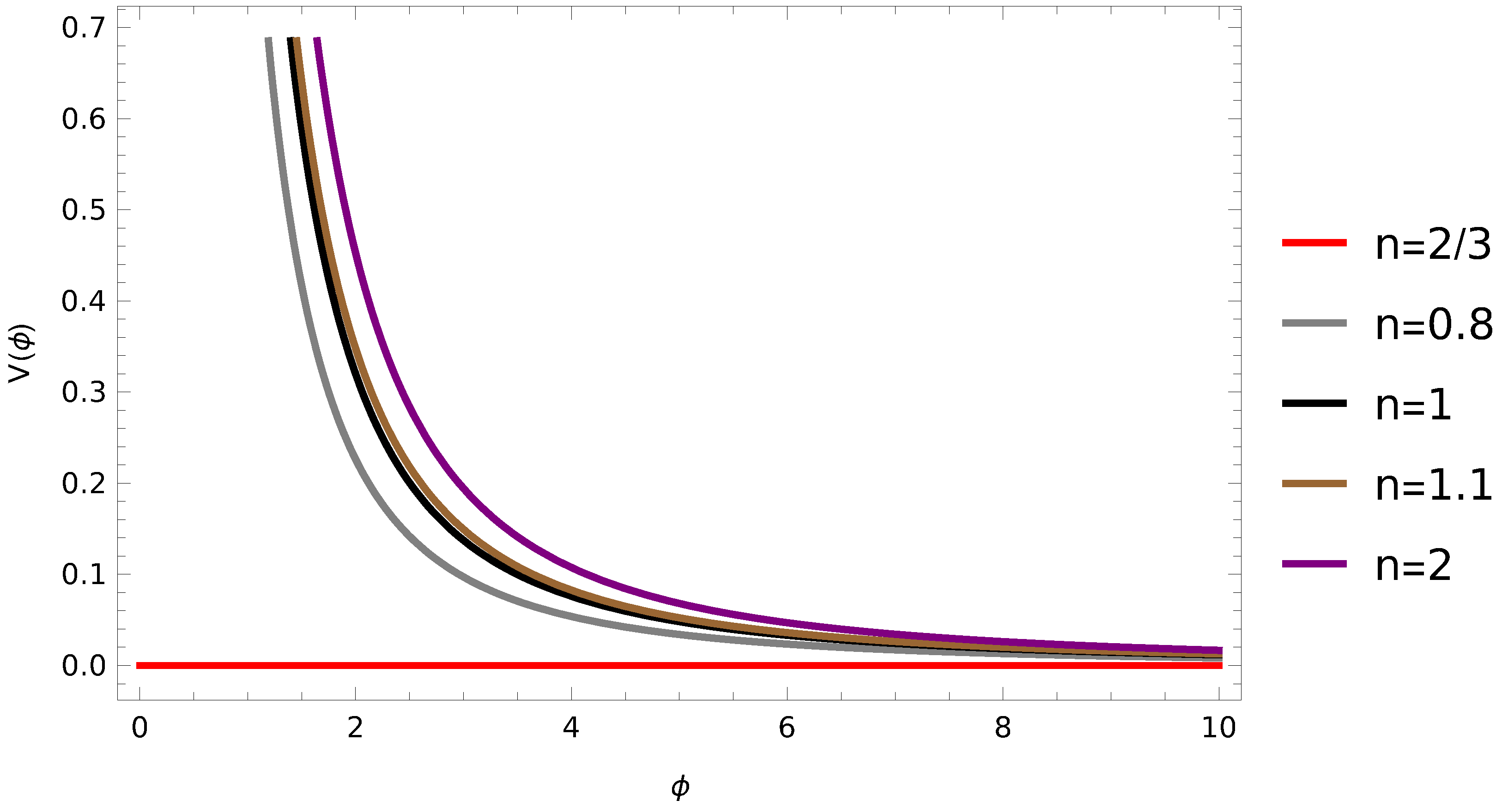
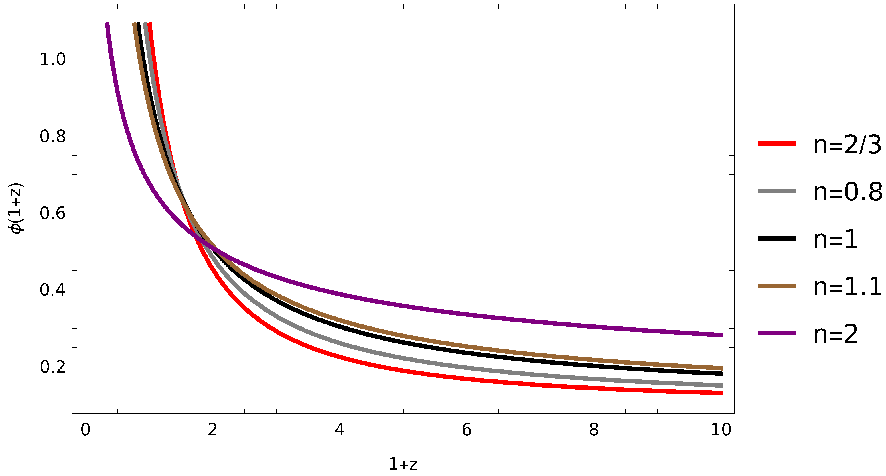
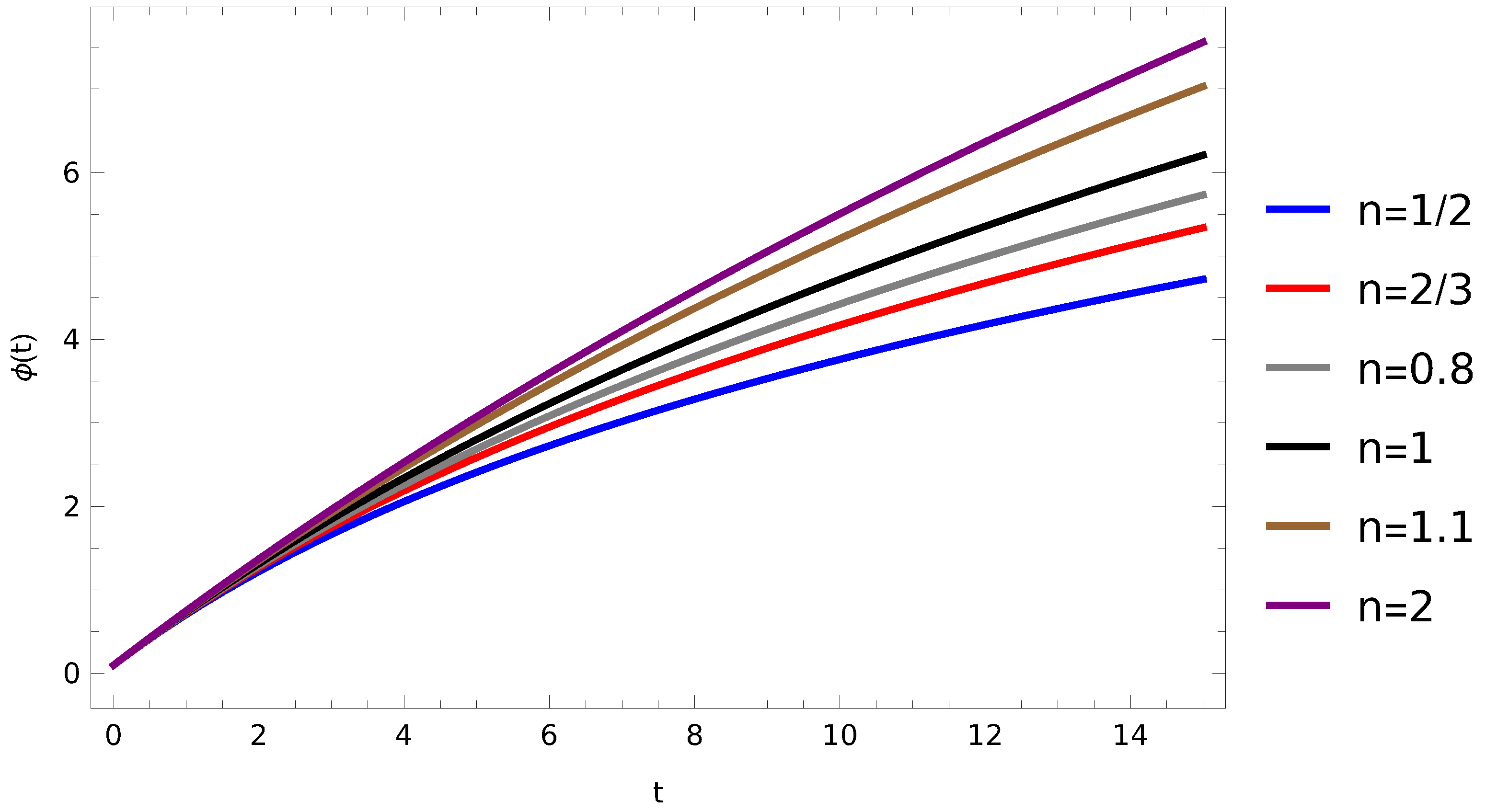
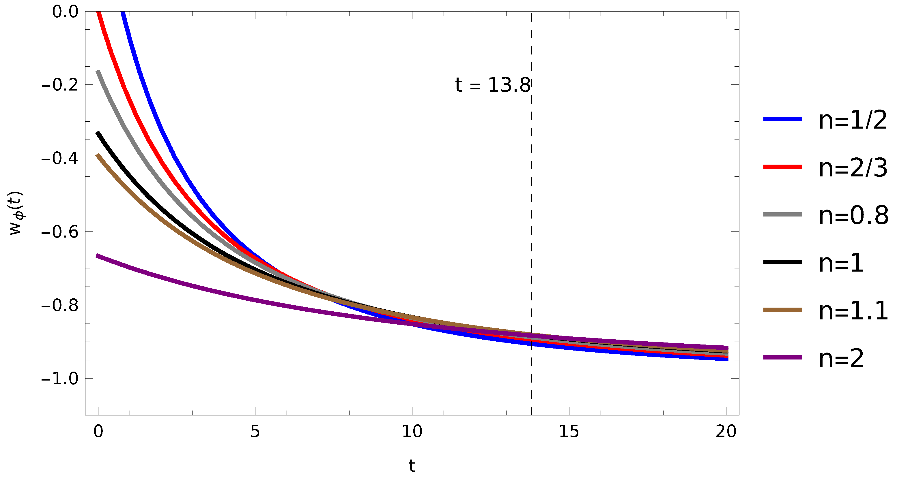
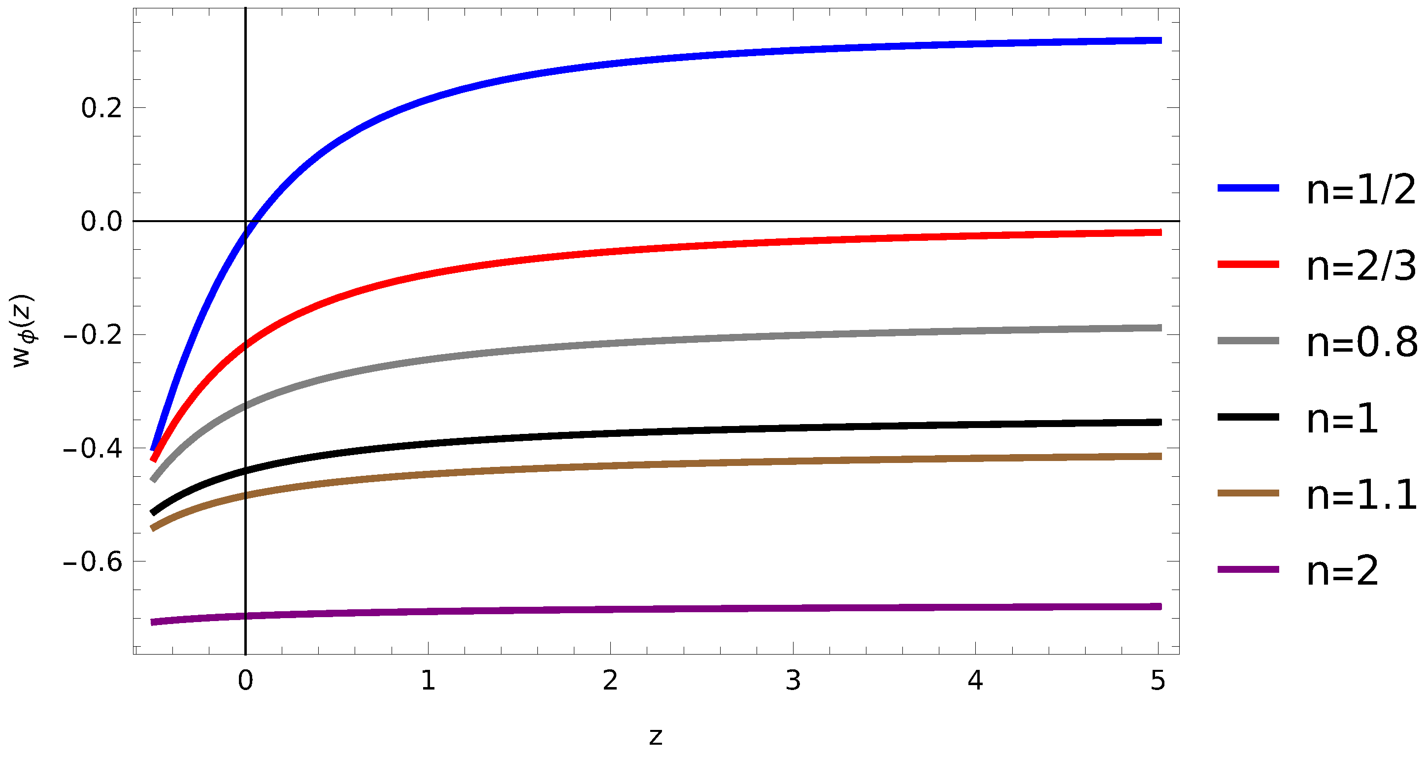
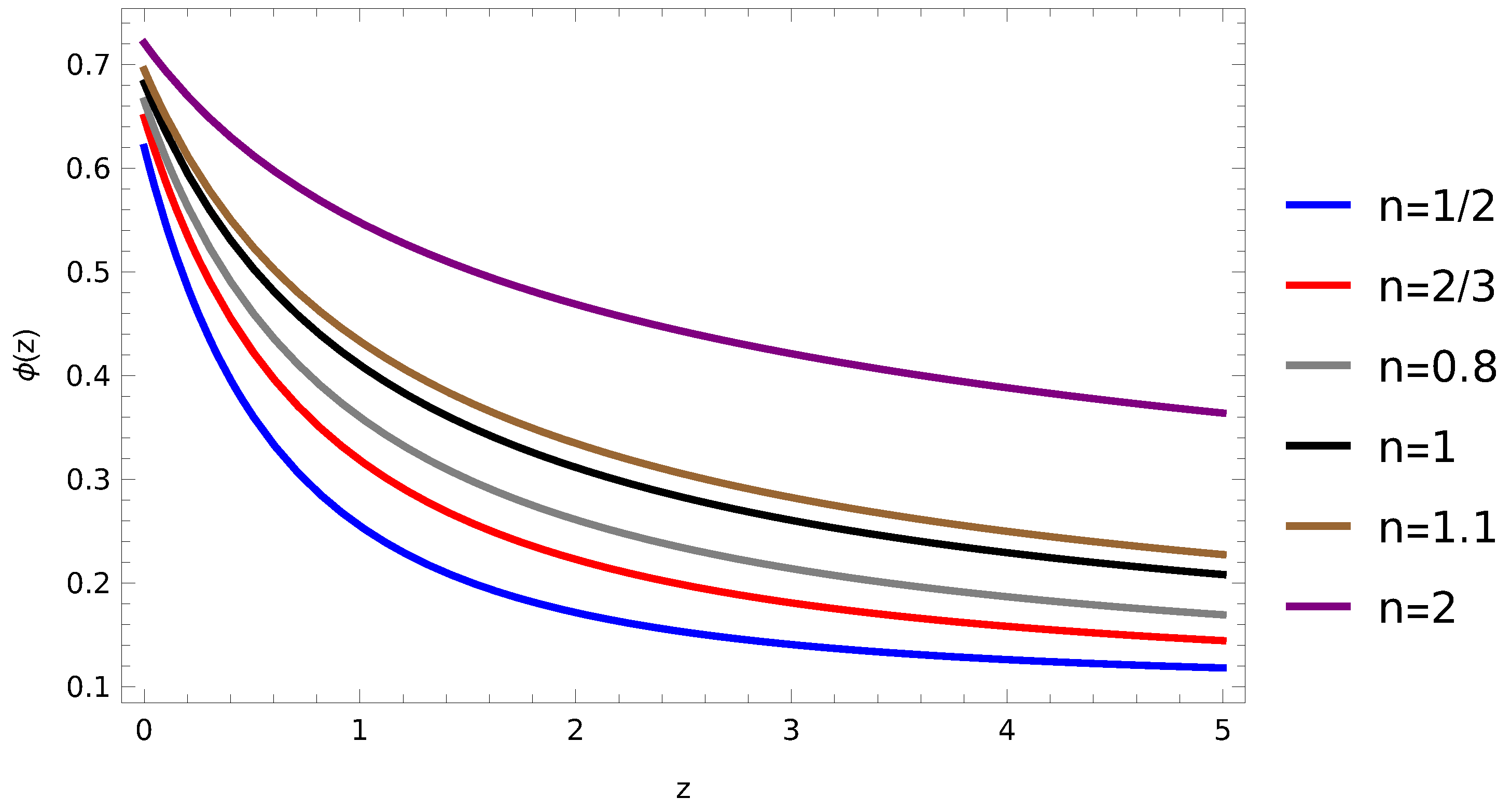
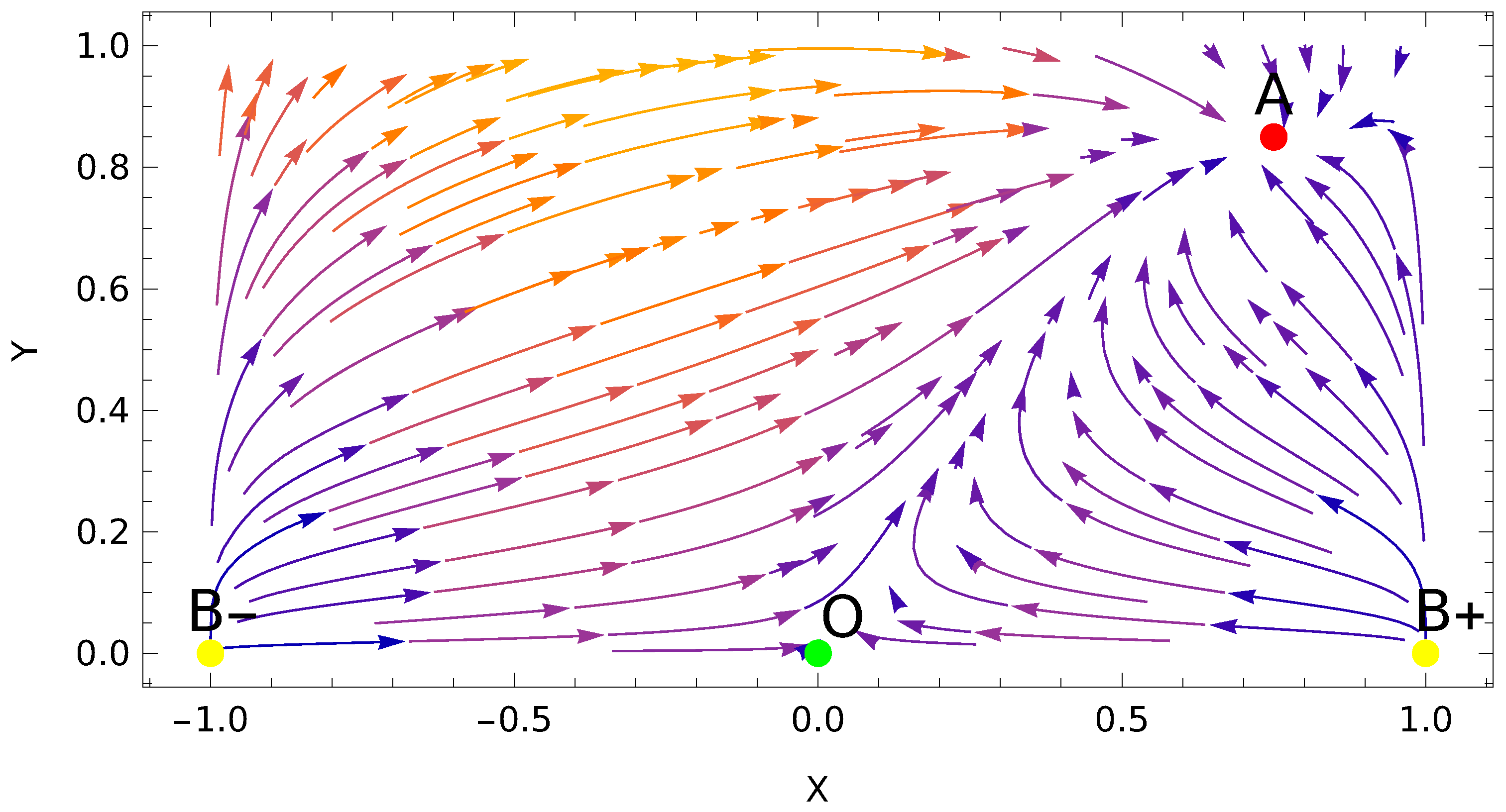
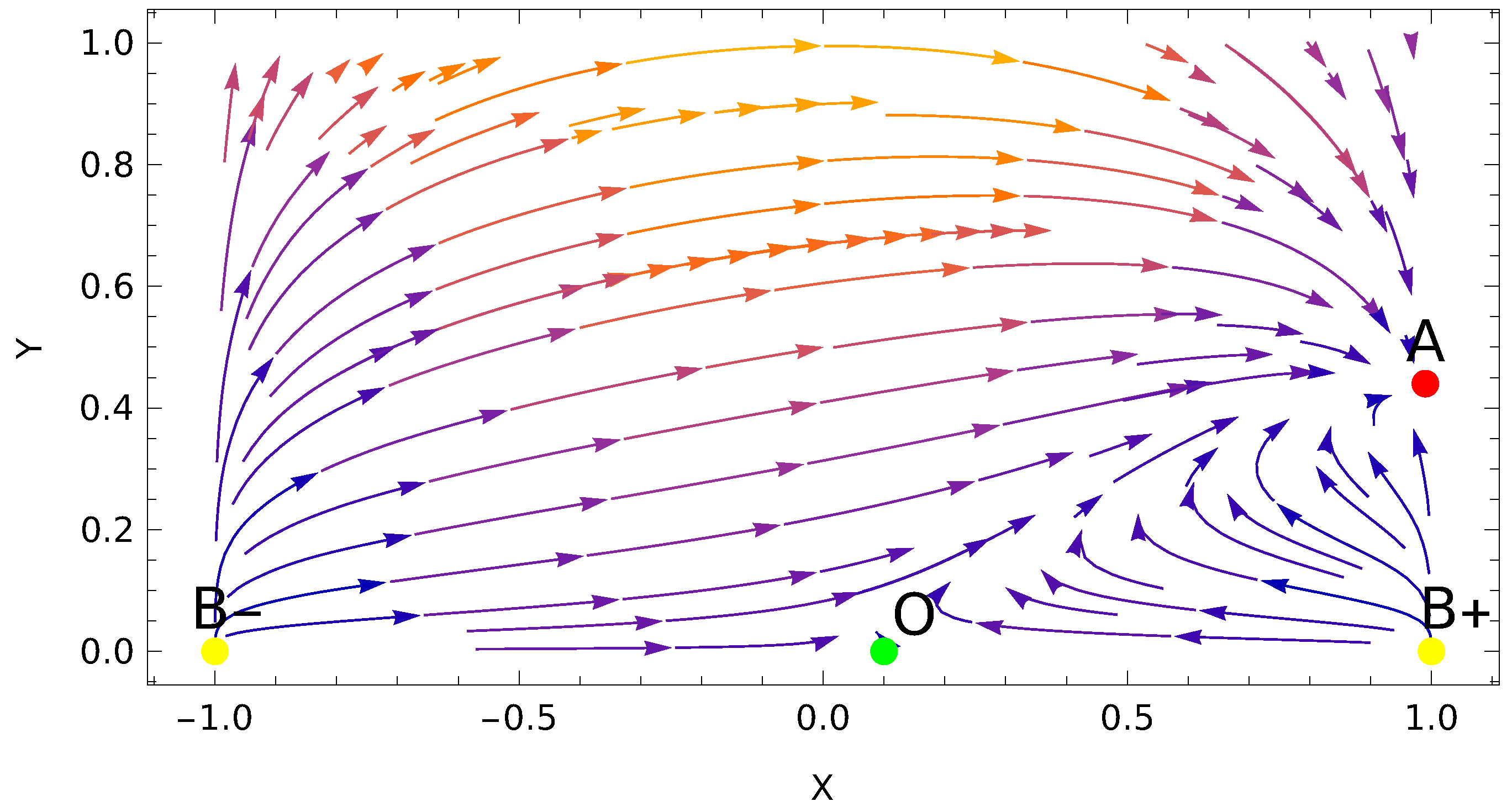
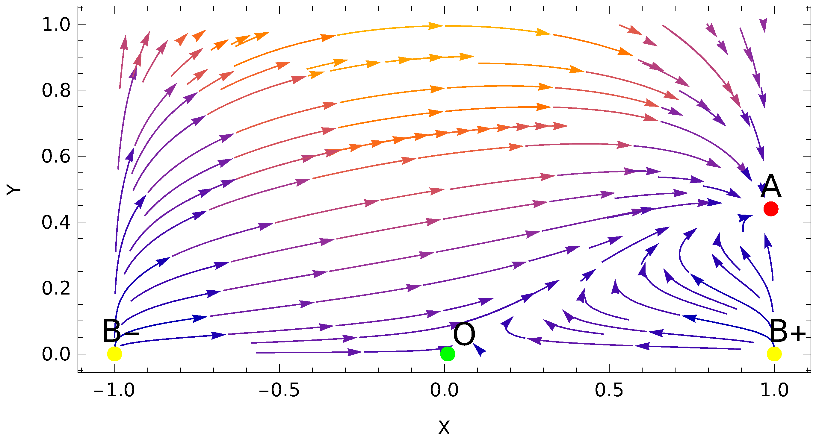
3. Dynamical Analysis at Inflection Point

In this section, we perform a dynamical analysis of our inflection point tachyon model. Dynamical analysis [82,83,84,85] is a powerful tool used to study the dynamics of a given model under consideration and its behaviour over time, thereby providing insights into its long-term behaviour. It allows us to analyze the contribution of various components of the universe, including dark matter, dark energy, and ordinary matter, by identifying and analyzing the critical points and their stability. The background equations governing the model are as follows:

$$H^2={\displaystyle \frac{{\kappa }^2}{3}}\rho$$

(39a)

$${\displaystyle \frac{\ddot{a}}{a}}={\displaystyle \frac{-{\kappa }^2}{6}}(\rho +3p)$$

(39b)

Here again, as mentioned earlier, $\rho$ and $p_m$ contain two components, namely scalar field and matter. We set the dimensionless variables [82] as follows:

$$X=\dot{\varphi }\equiv H{\varphi }^{\prime }$$

(40a)

$$Y={\displaystyle \frac{\kappa \sqrt{V}}{\sqrt{3}H}}$$

(40b)

$$\mathsf{\Gamma }={\displaystyle \frac{V(d^{2}V/d{\varphi }^2)}{{(dV/d\varphi )}^2}}$$

(40c)

Here, the scalar field has inverse mass dimensions and ${}^{\prime }$ signifies the derivative with respect to $\eta =loga$. In the above equation, the term $\Gamma$ naturally approaches zero at the inflection point of the potential. By definition, an inflection point is where the second derivative of the potential vanishes, i.e., $d^{2}V/d{\varphi }^2=0$. This condition ensures that the potential flattens out locally, allowing the scalar field to undergo slow roll. The slow-roll behaviour, in turn, facilitates a smooth transition between different cosmological phases, making the inflection point a crucial feature in models describing cosmic acceleration. The vanishing of $\Gamma$ at this point further simplifies the dynamical system.

$$\lambda =-{\displaystyle \frac{dV/d\varphi }{\kappa \sqrt{V^3}}}$$

(40d)

Upon introducing the inflection point from Equation (34) into Equation (40d), we obtain the following value of $\lambda$:

$$\lambda ={\displaystyle \frac{1}{\sqrt{2n}}}\left({\displaystyle \frac{3{\beta }^2}{2n}}+{\displaystyle \frac{2\beta }{3}}\sqrt{{\displaystyle \frac{3}{2n}}}\right){\left({\displaystyle \frac{4\beta }{3}}\sqrt{{\displaystyle \frac{3}{2n}}}+{\displaystyle \frac{3\beta (1-3n)}{4n^2}}\sqrt{{\displaystyle \frac{2n}{3}}}\right)}^{-3/2}$$

(41)

Here, we obtain an autonomous two-dimensional system which has been previously studied by [49]. Two other parameters (see Equation (40d)) still have $\varphi$ dependency; upon differentiating these aforementioned dimensionless equations, namely Equations (40a), (40b), and (40d) with respect to $\eta =loga$ and using Equations (39a) and (39b), one can obtain the following equations:

$$X^{\prime }={\displaystyle \frac{dX}{d\eta }}=(X^2-1)(3X-\lambda \sqrt{3}Y)$$

(42a)

$$Y^{\prime }={\displaystyle \frac{dY}{d\eta }}={\displaystyle \frac{-Y}{2}}\left(3Y^2{\displaystyle \frac{(1+w_m-X^2)}{\sqrt{1-X^2}}}-3(1+w_m)+\sqrt{3}\lambda XY\right)$$

(42b)

$${\lambda }^{\prime }={\displaystyle \frac{3\sqrt{3}}{2}}{\lambda }^{2}XY$$

(42c)

Using the following constraint equation:

$${\mathsf{\Omega }}_{\varphi }={\displaystyle \frac{Y^2}{\sqrt{1-X^2}}}$$

(43)

the equation of state and the energy density of the tachyonic scalar field, in terms of these dimensionless parameters, can be written as follows:

$$w_{\varphi }=X^2-1$$

(44)

$${\mathsf{\Omega }}_m=1-{\displaystyle \frac{Y^2}{\sqrt{1-X^2}}}\le 1$$

(45)

and the effective equation of motion can be written as follows:

$$w_{eff}=w_m\left(1-{\displaystyle \frac{Y^2}{\sqrt{1-X^2}}}\right)-Y^2\sqrt{1-X^2}$$

(46)

The critical points for Equations (40a) and (40b) are discussed below and are listed in

Table 1. The table shows the critical points of the system (40a)–(45) at the inflection point with $\lambda$.

X	Y	$\mathit{Existence}$	${\mathit{w}}_{\mathit{eff}}$	Stability
0	0	$\forall n,(1+w_m)$	$w_m$	Unstable Saddle point
		$w_m=1$	1	Stable Node
$\pm 1$	0	$\forall n,(1+w_m)$	−	Unstable Nodes
${\displaystyle \frac{Y_c\lambda }{\sqrt{3}}}$	$Y_c=\sqrt{{\displaystyle \frac{-{\lambda }^2+\sqrt{{\lambda }^4+36}}{6}}}$	$\forall (1+w_m),$	$-Y_c^2\sqrt{1-{\displaystyle \frac{{\lambda }^2{Y}_c^2}{3}}}+$	Stable node
		$0<n<1$	$w_m\left(1-{\displaystyle \frac{Y_c^2}{\sqrt{1-\frac{{\lambda }^2{Y}_c^2}{3}}}}\right)$

:

There are five critical points within the dynamical analysis at the inflection point, as shown in Figure 9 and discussed below:

(a.) Point O: For this critical point, $X=0$ and $Y=0$; the energy density of the tachyonic scalar field is revealed to be 0, thereby signifying the matter-dominated epoch. From the Friedmann constraint equation, Equation (45), we can see that ${\mathsf{\Omega }}_m=1$ and $w_{eff}=w_m$ again signify the matter-dominated epoch; thus, this origin point of the phase space refers to the unstable saddle point, which has the following eigenvalues:

$${\nu }_1=-3<0$$

(47)

and

$${\nu }_2={\displaystyle \frac{3}{2}}(w_m+1)$$

(48)

For this critical point, if $(1+w_m)>0$, the point is an unstable saddle point. This saddle point demonstrates attractor behaviour, as shown in Figure 9, and, at this point, the value of $w_{\varphi }=-1$ imitates the cosmological constant behaviour.

(b.) Point B_ : For this point, we obtain the following critical points: $X=-1$ and $Y=0$. At this critical point, the tachyonic equation of state vanishes, i.e., $w_{\varphi }=0$; we also obtain the following eigenvalues:

$${\nu }_1=6>0$$

(49a)

and

$${\nu }_2={\displaystyle \frac{3}{2}}(w_m+1)>0;if(1+w_m)>0$$

(49b)

Therefore, the critical point B_ is an unstable node representing the past attractor, but, here, the tachyon field behaves like dust-like matter, as in the case with $w_{\varphi }=0$ and $w_{eff}=w_m$.

(c.) Point B ${}_{+}$: X = 1, Y = 0. This point also represents an unstable node with the same eigenvalues as mentioned above, as follows:

$${\nu }_1=6>0$$

(50a)

and

$${\nu }_2={\displaystyle \frac{3}{2}}(w_m+1)>0;if(1+w_m)>0$$

(50b)

This point also shows the same past attractor behaviour, and the field shows dust-like behaviour, with $w_{eff}=w_m$.

(d.) Point A:$(X={\displaystyle \frac{\lambda Y_c}{\sqrt{3}}},Y_c=\sqrt{{\displaystyle \frac{-{\lambda }^2+\sqrt{{\lambda }^4+36}}{6}}})$ is the stable node, with the following eigenvalues:

$${\nu }_1=-3+{\displaystyle \frac{(-{\lambda }^4+{\lambda }^2\sqrt{{\lambda }^4+36})}{12}}$$

(51)

$${\nu }_2=-3(1+w_m)+2{\displaystyle \frac{(-{\lambda }^4+{\lambda }^2\sqrt{{\lambda }^4+36})}{12}}$$

(52)

We obtain a stable point when $(1+w_m)>{\displaystyle \frac{(-{\lambda }^4+{\lambda }^2\sqrt{{\lambda }^4+36})}{18}}$; for this case, ${\mathsf{\Omega }}_{\varphi }={\displaystyle \frac{3(-{\lambda }^2+\sqrt{{\lambda }^4+36})}{18\sqrt{1-\frac{-{\lambda }^4+\sqrt{{\lambda }^4+36}}{18}}}}$, thereby showing dark energy-like behaviour at this point. This stable point also depends on the values of n; as the value of n increases, this stable point is shifting more towards $X=1$, and this behaviour can be seen in the phase portraits for different values of n. The critical point A, as shown in Figure 9, Figure 10 and Figure 11, represents the stability of the derived dynamical system of equations and shows the accelerated expansion of the universe at the inflection point, which is incorporated in the system via the variable $\lambda$, and the field experiences accelerated expansion at a late time period.

4. Conclusions

In this paper, the evolution of a minimally coupled tachyonic scalar field at the inflection point has been investigated within an accelerating universe. The inflection point signifies a transition between regions of stability and instability and provides a flat region suitable for the ultra slow-roll approximation. In fact, inflection point models can also offer a robust framework for describing the inflationary phase as it can provide a prolonged period of slow-roll inflation. In this paper, the field’s dynamics have been investigated for different forms of expansion factors, and by considering a different form of scale factor, a form of potential is derived; only the mixed form of potential has shown the inflection point. We have mainly considered the following three categories of scale (expansion) factor: (a) power-law expansion ($a\left(t\right)=\alpha t^n$); (b) the exponential form ($a\left(t\right)=\gamma e^{\beta t}$); and (c) the mixed form ($a\left(t\right)=\eta t^n{e}^{\beta t}$). For all these categories, the potentials and the corresponding possible inflection points have been calculated, and the dynamical system of equations for the model has been obtained. Out of these three categories, the mixed form shows inflection at ${\varphi }_{inflection}$, as given in Equation (34), and, near this point, under slow roll approximation, the evolution of the scalar field with cosmic time (t) and cosmological redshift (z) shows the accelerated expansion of the universe at late time periods near the inflection point. Figure 8 also indicates that a potential with an inflection point can provide a near-flat region for the field to slow roll, which may derive the accelerated cosmic expansion.

In Section 3, the dynamical analysis carried out shows that the critical point A, as shown in Figure 9, Figure 10 and Figure 11, represents the stability of the derived dynamical system of equations and shows the accelerated expansion of the universe at an inflection point, which is incorporated in the system via the variable $\lambda$, and the field demonstrates accelerated expansion at late time periods.

In addition to the research currently being carried out, it is important for future works to study the inflection point of scalar field models in the presence of quantum gravity effects. In particular, scalar field dynamics play a significant role in the post-bounce scenario of loop quantum cosmology as it gives rise to an inflationary solution [86,87]. Our future pursuits will include the investigation of how inflection points are affected due to quantum geometric correction for scalar fields.

References

1. Riess, A.G.; Filippenko, A.V.; Challis, P.; Clocchiatti, A.; Diercks, A.; Garnavich, P.M.; Gilliland, R.L.; Hogan, C.J.; Jha, S.; Kirshner, R.P.; et al. Observational evidence from supernovae for an accelerating universe and a cosmological constant. Astron. J. 1998, 116, 1009. [Google Scholar] [CrossRef]
2. Perlmutter, S.; Aldering, G.; Goldhaber, G.; Knop, R.A.; Nugent, P.; Castro, P.G.; Deustua, S.; Fabbro, S.; Goobar, A.; Groom, D.E.; et al. [The Supernova Cosmology Project] Measurements of Ω and Λ from 42 high-redshift supernovae. Astrophys. J. 1999, 517, 565. [Google Scholar] [CrossRef]
3. Spergel, D.N.; Verde, L.; Peiris, H.V.; Komatsu, E.; Nolta, M.R.; Bennett, C.L.; Halpern, M.; Hinshaw, G.; Jarosik, N.; Kogut, A.; et al. First-year Wilkinson Microwave Anisotropy Probe (WMAP)* observations: Determination of cosmological parameters. Astrophys. J. 2003, 148, 175. [Google Scholar] [CrossRef]
4. Seo, H.; Eisenstein, D.J. Probing dark energy with baryonic acoustic oscillations from future large galaxy redshift surveys. Astrophys. J. 2003, 598, 720. [Google Scholar] [CrossRef]
5. Blake, C.; Glazebrook, K. Probing dark energy using baryonic oscillations in the galaxy power spectrum as a cosmological ruler. Astrophys. J. 2003, 594, 665. [Google Scholar] [CrossRef]
6. Jarosik, N.; Bennett, C.L.; Dunkley, J.; Gold, B.; Greason, M.R.; Halpern, M.; Hill, R.S.; Hinshaw, G.; Kogut, A.; Komatsu, E.; et al. Seven-year wilkinson microwave anisotropy probe (WMAP*) observations: Sky maps, systematic errors. and basic results, Astrophys. J. 2011, 192, 18. [Google Scholar] [CrossRef]
7. Aghanim, N.; Akrami, Y.; Ashdown, M.; Aumont, J.; Baccigalupi, C.; Ballardini, M.; Banday, A.J.; Barreiro, R.B.; Bartolo, N.; Basak, S.; et al. [Planck Collaboration] Planck 2018 results VI. Cosmological parameters. Astron. Astrophys. 2020, 641, A6. [Google Scholar]
8. Aghanim, N.; Akrami, Y.; Ashdown, M.; Aumont, J.; Baccigalupi, C.; Ballardini, M.; Banday, A.J.; Barreiro, R.B.; Bartolo, N.; Basak, S.; et al. [Planck Collaboration] Planck 2018 results I. Overview and the cosmological legacy of Planck. Astron. Astrophys. 2020, 641, A1. [Google Scholar]
9. Knop, R.A.; Aldering, G.; Amanullah, R.; Astier, P.; Blanc, G.; Burns, M.S.; Conley, A.; Deustua, S.E.; Doi, M.; Ellis, R.; et al. [The Supernova Cosmology Project] New constraints on Ωm, ΩΛ, and w from an independent set of 11 high-redshift supernovae observed with the Hubble Space Telescope. Astrophys. J. 2003, 598, 102. [Google Scholar] [CrossRef]
10. Riess, A.G.; Strolger, L.G.; Tonry, J.; Casertano, S.; Ferguson, H.C.; Mobasher, B.; Challis, P.; Filippenko, A.V.; Jha, S.; Li, W.; et al. Type Ia supernova discoveries at z>1 from the Hubble Space Telescope: Evidence for past deceleration and constraints on dark energy evolution. Astrophys. J. 2004, 607, 665. [Google Scholar] [CrossRef]
11. Ellis, G.F.R.; Platts, E.; Sloan, D.; Weltman, A. Current observations with a decaying cosmological constant allow for chaotic cyclic cosmology. J. Cosmol. Astropart. Phys. 2016, 4, 026. [Google Scholar] [CrossRef]
12. Patil, T.; Panda, S.; Sharma, M. Dynamics of interacting scalar field model in the realm of chiral cosmology. Eur. Phys. J. C 2023, 83, 131. [Google Scholar] [CrossRef]
13. Szydłowski, M.S.; Stachowski, A. Cosmology with decaying cosmological constant—Exact solutions and model testing. J. Cosmol. Astropart. Phys. 2015, 10, 066. [Google Scholar] [CrossRef]
14. Bisabr, Y.; Salehi, H. Mechanism for a decaying cosmological constant. Class. Quantum Grav. 2002, 19, 2369. [Google Scholar] [CrossRef]
15. Fujii, Y.; Nishioka, T. Model of a decaying cosmological constant. Phys. Rev. D 1990, 42, 361. [Google Scholar] [CrossRef]
16. Bull, P.; Akrami, Y.; Adamek, J.; Baker, T.; Bellini, E.; Jiménez, J.B.; Bentivegna, E.; Camera, S.; Clesse, S.; Davis, J.H.; et al. Beyond ΛCDM: Problems, solutions, and the road ahead. Phys. Dark Universe 2016, 12, 56. [Google Scholar] [CrossRef]
17. Perivolaropoulos, L.; Skara, F. Challenges for ΛCDM: An update. New Astron. Rev. 2022, 95, 101659. [Google Scholar] [CrossRef]
18. Popolo, A.D.; Delliou, M.L. Small scale problems of the ΛCDM model: A short review. Galaxies 2017, 5, 17. [Google Scholar] [CrossRef]
19. Weinberg, S. The cosmological constant problem. Rev. Mod. Phys. 1989, 61, 1. [Google Scholar] [CrossRef]
20. Astashenok, A.V.; Popolo, A.D. Cosmological measure with volume averaging and the vacuum energy problem. Class. Quantum Gravity 2012, 29, 085014. [Google Scholar] [CrossRef]
21. Ratra, B.; Peebles, P.J.E. Cosmological consequences of a rolling homogeneous scalar field. Phys. Rev. D 1988, 37, 3406. [Google Scholar] [CrossRef] [PubMed]
22. Escamilla-Rivera, C.; Najera, A. Dynamical dark energy models in the light of gravitational-wave transient catalogues. J. Cosmol. Astropart. Phys. 2022, 3, 060. [Google Scholar] [CrossRef]
23. Zhao, G.B.; Raveri, M.; Pogosian, L.; Wang, Y.; Crittenden, R.G.; Handley, W.J.; Percival, W.J.; Beutler, F.; Brinkmann, J.; Chuang, C.H.; et al. Dynamical dark energy in light of the latest observations. Nat. Astron. 2017, 1, 627. [Google Scholar] [CrossRef]
24. Mainini, R.; Macciò, A.V.; Bonometto, S.A.; Klypin, A. Modeling dynamical dark energy. Astrophys. J. 2003, 599, 24. [Google Scholar] [CrossRef]
25. Brax, P.; Burrage, C.; Englert, C.; Spannowsky, M. LHC signatures of scalar dark energy. Phys. Rev. D 2016, 94, 084054. [Google Scholar] [CrossRef]
26. Copeland, E.J.; Sami, M.; Tsujikawa, S. Dynamics of dark energy. Int. J. Mod. Phys. D 2006, 15, 1753. [Google Scholar] [CrossRef]
27. Adame, A.G. et al. [The DESI collaboration] DESI 2024 VI: Cosmological constraints from the measurements of baryon acoustic oscillations. J. Cosmol. Astropart. Phys. 2025, 2025, 021. [Google Scholar] [CrossRef]
28. Lodha, K. et al. [DESI Collaboration] DESI 2024: Constraints on physics-focused aspects of dark energy using DESI DR1 BAO data. Phys. Rev. D. 2025, 111, 023532. [Google Scholar] [CrossRef]
29. Giarè, W.; Sabogal, M.A.; Nunes, R.C.; Valentino, E.D. Interacting dark energy after DESI baryon acoustic oscillation measurements. Phys. Rev. D. 2024, 133, 251003. [Google Scholar] [CrossRef]
30. Alestas, G.; Caldarola, M.; Kuroyanagi, S.; Nesseris, S. DESI constraints on α-attractor inflationary models. arXiv 2024, arXiv:2410.00827. [Google Scholar] [CrossRef]
31. Andriot, D. Quintessence: An analytical study, with theoretical and observational applications. arXiv 2024, arXiv:2410.17182. [Google Scholar]
32. Andriot, D. Exponential quintessence: Curved, steep and stringy? J. High Energy Phys. 2024, 2024, 1–60. [Google Scholar] [CrossRef]
33. Bhattacharya, S. Cosmological constraints on curved quintessence. J. Cosmol. Astropart. Phys. 2024, 2024, 073. [Google Scholar] [CrossRef]
34. Verma, M.M.; Pathak, S.D. Cosmic expansion driven by real scalar field for different forms of potential. Astrophys. Space Sci. 2014, 350, 381. [Google Scholar] [CrossRef]
35. Verma, M.M.; Pathak, S.D. The BICEP2 data and a single Higgs-like interacting scalar field. Anisotropic bouncing scenario in F (X)- V (ϕ) F(X)-V(ϕ) model. Int. J. Mod. Phys. D 2014, 23, 1450075. [Google Scholar] [CrossRef]
36. Panda, S.; Sharma, M. Gauging universe expansion via scalar fields. Astrophys. Space Sci. 2016, 361, 1–8. [Google Scholar]
37. Kumar, S.; Pathak, S.D.; Khlopov, M. Dynamics of Quasi-Exponential Expansion: Scalar Field Potential Insights. Int. J. Theor. Phys. 2024, 63, 238. [Google Scholar] [CrossRef]
38. Verma, M.M.; Pathak, S.D. Shifted cosmological parameter and shifted dust matter in a two-phase tachyonic field universe. Astrophys. Space Sci. 2013, 344, 505. [Google Scholar] [CrossRef]
39. Kumar, D.R.; Pathak, S.D.; Ojha, V.K. Gauging universe expansion via scalar fields. Chin. Phys. C 2023, 47, 055102. [Google Scholar] [CrossRef]
40. Johri, V.B. Phantom cosmologies. Phys. Rev. D 2004, 70, 041303R. [Google Scholar] [CrossRef]
41. Johri, V.B. Search for tracker potentials in quintessence theory. Class. Quantum Gravity 2002, 19, 5959. [Google Scholar] [CrossRef]
42. Johri, V.B. Genesis of cosmological tracker fields. Phys. Rev. D 2001, 63, 103504. [Google Scholar] [CrossRef]
43. Kumar, S.; Pathak, S.D.; Zhang, X. Deciphering star formation dynamics with coupled ϕCDM. Europhys. Lett. 2025, 149. [Google Scholar]
44. Gialamas, I.D.; Hütsi, G.; Kannike, K.; Racioppi, A.; Raidal, M.; Vasar, M.; Veermäe, H. Interpreting DESI 2024 BAO: Late-time dynamical dark energy or a local effect? Phys. Rev. D. 2025, 111, 043540. [Google Scholar] [CrossRef]
45. Amendola, L. Coupled quintessence. Phys. Rev. D 2000, 64, 043511. [Google Scholar] [CrossRef]
46. Park, C.G.; Ratra, B. Is excess smoothing of Planck CMB ansiotropy data partially responsible for evidence for dark energy dynamics in other w(z)CDM parametrizations? arXiv 2025, arXiv:2501.03480. [Google Scholar]
47. Bhattacharya, S.; Borghetto, G.; Malhotra, A.; Parameswaran, S.; Tasinato, G.; Zavala, I. Cosmological tests of quintessence in quantum gravity. arXiv 2024, arXiv:2410.21243. [Google Scholar]
48. Bagla, J.S.; Jassal, H.K.; Padmanabhan, T. Cosmology with tachyon field as dark energy. Phys. Rev. D. 2003, 67, 063504. [Google Scholar] [CrossRef]
49. Copeland, E.J.; Garousi, M.R.; Sami, M.; Tsujikawa, S. What is needed of a tachyon if it is to be the dark energy? Phys. Rev. D. 2005, 71, 043003. [Google Scholar] [CrossRef]
50. Padmanabhan, T. Accelerated expansion of the universe driven by tachyonic matter. Phys. Rev. D. 2002, 66, 021301. [Google Scholar] [CrossRef]
51. Choudhury, S.; Mazumdar, A. An accurate bound on tensor-to-scalar ratio and the scale of inflation. Nucl. Phys. B 2014, 9, 386. [Google Scholar] [CrossRef]
52. Salucci, P.; Esposito, G.; Lambiase, G.; Battista, E.; Benetti, M.; Bini, D.; Boco, L.; Sharma, G.; Bozza, V.; Buoninfante, L. Einstein, Planck and Vera Rubin: Relevant encounters between the Cosmological and the Quantum Worlds. Front. Phys. 2021, 8, 603190. [Google Scholar] [CrossRef]
53. Allahverdi, R.; Dutta, B.; Mazumdar, A. Attraction towards an inflection point inflation. Phys. Rev. D 2008, 78, 063507. [Google Scholar] [CrossRef]
54. Battista, E. Nonsingular bouncing cosmology in general relativity: Physical analysis of the spacetime defect. Class. Quantum Grav. 2021, 19, 195007. [Google Scholar] [CrossRef]
55. Bai, Y.; Stolarski, D. Dynamical inflection point inflation. J. Prof. Assoc. Cactus Dev. 2021, 3, 091. [Google Scholar] [CrossRef]
56. Choudhury, S.; Mazumdar, A.; Pukartas, E. Constraining N=1 supergravity inflationary framework with non-minimal Kähler operators. J. High Energy Phys. 2014, 4, 1–27. [Google Scholar] [CrossRef]
57. Enqvist, K.; Mazumdar, A. Cosmological consequences of MSSM flat directions. Phys. Rep. 2003, 380, 99–234. [Google Scholar] [CrossRef]
58. Enqvist, K.; Jokinen, A.; Mazumdar, A. Dynamics of minimal supersymmetric standard model flat directions consisting of multiple scalar fields. J. Cosmol. Astropart. Phys. 2004, 1, 008. [Google Scholar] [CrossRef]
59. Enqvist, K.; Mazumdar, A.; Stephens, P. Inflection point inflation within supersymmetry. J. Cosmol. Astropart. Phys. 2010, 2010, 020. [Google Scholar] [CrossRef]
60. Allahverdi, R.; Enqvist, K.; Garcia-Bellido, J.; Jokinen, A.; Mazumdar, A. MSSM flat direction inflation: Slow roll, stability, fine-tuning and reheating. J. Cosmol. Astropart. Phys. 2007, 2007, 019. [Google Scholar] [CrossRef]
61. Mazumdar, A.; Rocher, J. Particle physics models of inflation and curvaton scenarios. Phys. Reps. 2011, 497, 85–215. [Google Scholar] [CrossRef]
62. Choudhury, S.; Mazumdar, A. Primordial blackholes and gravitational waves for an inflection-point model of inflation. Phys. Lett. B 2014, 733, 270–275. [Google Scholar] [CrossRef]
63. Choudhury, S.; Mazumdar, A. Reconstructing inflationary potential from BICEP2 and running of tensor modes. arXiv 2014, arXiv:1403.5549. [Google Scholar]
64. Allahverdi, R.; Enqvist, K.; Garcia-Bellido, J.; Mazumdar, A. Gauge-invariant inflaton in the minimal supersymmetric standard model. Phys. Rev. Lett. 2006, 97, 191304. [Google Scholar] [CrossRef]
65. Choi, S.M.; Lee, H.M. Inflection point inflation and reheating. Eur. Phys. J. C 2016, 76, 1–15. [Google Scholar] [CrossRef]
66. Dimopoulos, K.; Owen, C.; Racioppi, A. Loop inflection-point inflation. Astropart. Phys. 2018, 103, 16–20. [Google Scholar] [CrossRef]
67. Kaur, J.; Pathak, S.D.; Khlopov, M.Y. Inflection point of coupled quintessence. Astropart. Phys. 2024, 157, 102926. [Google Scholar] [CrossRef]
68. Iacconi, L.; Assadullahi, H.; Fasiello, M.; Wands, D. Revisiting small-scale fluctuations in α-attractor models of inflation. J. Cosmol. Astropart. Phys. 2022, 6, 007. [Google Scholar] [CrossRef]
69. Blanco-Pillado, J.J.; Gomez-Reino, M.; Metallinos, K. Accidental inflation in the landscape. J. Cosmol. Astropart. Phys. 2013, 2, 034. [Google Scholar] [CrossRef]
70. Kefala, K.; Kodaxis, G.P.; Stamou, I.D.; Tetradis, N. Features of the inflaton potential and the power spectrum of cosmological perturbations. Phys. Rev. D 2021, 104, 023506. [Google Scholar] [CrossRef]
71. Storm, S.D.; Scherrer, R.J. Observational constraints on inflection point quintessence with a cubic potential. Phys. Lett. B 2022, 829, 137126. [Google Scholar] [CrossRef]
72. Cerezo, R.; Rosa, J.G. Warm inflection. J. High Energy Phys. 2013, 2013, 24. [Google Scholar] [CrossRef]
73. Hotchkiss, S.; Mazumdar, A.; Nadathur, S. Inflection point inflation: WMAP constraints and a solution to the fine tuning problem. J. Cosmol. Astropart. Phys. 2011, 6, 002. [Google Scholar] [CrossRef]
74. Chang, H.Y.; Scherrer, R.J. Inflection point quintessence. Phys. Rev. D 2013, 88, 083003. [Google Scholar] [CrossRef]
75. Gorini, V.; Kamenshchik, A.; Moschella, U.; Pasquier, V. Tachyons, scalar fields, and cosmology. Phys. Rev. D. 2004, 69, 123512. [Google Scholar] [CrossRef]
76. Singh, A.; Jassal, H.K.; Harma, M.S. Perturbations in tachyon dark energy and their effect on matter clustering. J. Cosmol. Astropart. Phys. 2020, 2020, 008. [Google Scholar] [CrossRef]
77. Bamba, K.; Capozziello, S.; Nojiri, S.; Odintsov, S.D. Dark energy cosmology: The equivalent description via different theoretical models and cosmography tests. Astrophys. Space Sci. 2012, 342, 155–228. [Google Scholar] [CrossRef]
78. Piao, Y.S.; Huang, Q.G.; Zhang, X.; Zhang, Y.Z. Non-minimally coupled tachyon and inflation. Phys. Lett. B. 2003, 570, 1. [Google Scholar] [CrossRef]
79. Mezo, I. The Lambert W Function: Its Generalizations and Applications, 1st ed.; Chapman and Hall/CRC: New York, NY, USA, 2022. [Google Scholar] [CrossRef]
80. Kalugin, G.A. Analytical Properties of the Lambert W Function. Doctoral Thesis, Western University, London, ON, Canada, 2011. [Google Scholar]
81. Thompson, R.I. Non-Canonical Dark Energy Parameter Evolution in a Canonical Quintessence Cosmology. Universe 2024, 10, 356. [Google Scholar] [CrossRef]
82. Bahamonde, S.; Böhmer, C.G.; Carloni, S.; Copeland, E.J.; Fang, W.; Tamanini, N. Dynamical systems applied to cosmology: Dark energy and modified gravity. Phys. Rep. 2018, 775, 1–122. [Google Scholar] [CrossRef]
83. Pathak, S.D.; Mishra, S.S.; Kaur, J.; Khlopov, M. Chapter 3—Application of Dynamical System Analysis in Cosmology, Advances in Computational Methods and Modeling for Science and Engineering; Morgan Kaufmann: Burlington, MA, USA, 2025; pp. 37–47. ISBN 9780443300127. [Google Scholar]
84. Coley, A.A. Dynamical Systems and Cosmology; Springer Science Business Media: Berlin/Heidelberg, Germany, 2003. [Google Scholar]
85. Arrowsmith, D.K. An Introduction to Dynamical Systems; Cambridge University Press: Cambridge, UK, 1990. [Google Scholar]
86. Sharma, M.; Shahalam, M.; Wu, Q.; Wang, A. Preinflationary dynamics in loop quantum cosmology: Monodromy Potential. J. Cosmol. Astropart. Phys. 2018, 2018, 003. [Google Scholar] [CrossRef]
87. Shahalam, M.; Shahalam, M.; Wu, Q.; Wang, A. Preinflationary dynamics in loop quantum cosmology: Power-law potentials. Phys. Rev. D 2017, 96, 123533. [Google Scholar] [CrossRef]
Figure 1. The plot shows the variation of ϕ with potential V ( ϕ ) for different values of the exponent factor n ( n = 2 / 3 , n = 0.8 , n = 1 , n = 1.1 , and n = 2 ) for fixed value of ϕ 0 = 0.1 .
Universe 11 00131 g001
Figure 2. The plot shows the evolution of ϕ with cosmological redshift z for different values of the exponent factor n ( n = 2 / 3 , n = 0.8 , n = 1 , n = 1.1 , and n = 2 ), with the normalization constant α = 1 (for simplicity) and ϕ 0 0.1 .
Universe 11 00131 g002
Figure 3. The plot shows the evolution of ϕ with cosmic time t for different values of n, β = 0.1 , and ϕ 0 = 0.1 .
Universe 11 00131 g003
Figure 4. The plot shows the evolution of w ϕ with cosmic time t (Gyr) for different values of n, β = 0.1 , and ϕ 0 = 0.1 .
Universe 11 00131 g004
Figure 5. The plot shows the variation in the scalar field ϕ with respect to the potential V ( ϕ ) for different sets of values of n with a fixed value of β < < 1 , specifically β = 0.1 and ϕ 0 = 0.1 .
Universe 11 00131 g005
Figure 6. The plot shows the variation in equation of state w ϕ with respect to cosmological redshift z for different sets of values of n ( n = 1 / 2 , n = 2 / 3 , n = 0.8 , n = 1 , n = 1.1 and n = 2 from top to bottom) with a fixed value of β < < 1 , specifically β = 0.1 and ϕ 0 = 0.1 . Here in plot vertical solid black line represents the present epoch with z = 0 while the horizontal blacksolid line represents null value of equation of state parameter w ϕ .
Universe 11 00131 g006
Figure 7. The plot shows the variation in the scalar field ϕ with respect to cosmological redshift z for different sets of values of n with a fixed value of β < < 1 , specifically β = 0.1 and ϕ 0 = 0.1 .
Universe 11 00131 g007
Figure 8. The plot shows the variation in potential V ( ϕ ( z ) ) with respect to cosmological redshift z for different sets of values of n with a fixed value of β < < 1 , specifically β = 0.1 , η = 1 , and ϕ 0 = 0.1 .
Universe 11 00131 g008
Figure 9. A phase portrait of the dynamical system for n = 1 / 3 with λ 1 and w m = 0 , near the inflection point ϕ i n f l e c t i o n with β < < 1 ( β = 0.1 ). In plot A, O, B and B + represents the critical points. Here, stable point A in the phase space shows the region where the universe undergoes accelerated expansion.
Universe 11 00131 g009
Figure 10. Phase portrait of the dynamical system for n = 2 / 3 with λ > 1 and w m = 0 , near the inflection point ϕ i n f l e c t i o n with β < < 1 ( β = 0.1 ). In plot A, O, B and B + represents the critical points. The stable point A in the phase space shows the region where universe undergoes accelerated expansion; however, because of the increase in n, point A is shifting towards X∼1.
Universe 11 00131 g010
Figure 11. Phase portrait of the dynamical system for n = 0.8 with λ 5 and w m = 0 , near the inflection point ϕ i n f l e c t i o n with β < < 1 ( β = 0.1 ). In plot A, O, B and B + represents the critical points. The stable point A in the phase space shows the region where universe undergoes accelerated expansion; however, because of the increase in n, point A is shifting more towards 1.
Universe 11 00131 g011