Determining the Scale Length and Height of the Milky Way’s Thick Disc Using RR Lyrae

Abstract

Using the RR Lyrae surveys Gaia DR3 Specific Objects Study, PanSTARRS1 and ASAS-SN-II, we determine the Milky Way’s thick disc scale length and scale height as well as the radial scale length of the galaxy’s inner halo. We use a Bayesian approach to estimate these values using two independent techniques: Markov chain Monte Carlo sampling, and importance nested sampling. We consider two vertical density profiles for the thick disc. In the exponential model, the scale length of the thick disc is $h_R={2.14}_{-0.17}^{+0.19}$ kpc, and its scale height is $h_z={0.64}_{-0.06}^{+0.06}$ kpc. In the squared hyperbolic secant profile $sec{h}^2$, those values are correspondingly $h_R={2.10}_{-0.17}^{+0.19}$ kpc and $h_z={1.02}_{-0.08}^{+0.09}$ kpc. The density distribution of the inner halo can be described as a power law function with the exponent $n=-{2.35}_{-0.05}^{+0.05}$ and flattening $q={0.57}_{-0.02}^{+0.02}$. We also estimate the halo to disc concentration ratio as $\gamma ={0.19}_{-0.02}^{+0.02}$ for the exponential disc and $\gamma ={0.32}_{-0.03}^{+0.03}$ for the $sec{h}^2$ disc.

1. Introduction

The study of galactic structures is one of the most important topics of modern astrophysics since it provides insights into the formation of the Milky Way galaxy. Among all the galactic components, the precise structure of the thick disc of the Milky Way galaxy plays an important role in influencing the distribution and equilibrium rotation of the Milky Way’s thin and thick discs, as well as in inferring the dark matter density distribution in the solar neighborhood and inner halo. Thick discs were first discovered in external galaxies by Burstein [1]. The existence of the thick disc in the Milky Way galaxy was confirmed immediately after by Gilmore and Reid [2].

The presence of the galactic thick disc can be confirmed not only by the vertical density distribution of the disc. Kinematically, the rotation of the thick disc lags behind that of the thin disc by about 50 km/s [3]. The thick disc is also older, metal-poorer and richer in alpha elements compared to the thin disc [3,4,5,6,7]. The knowledge of the radial and vertical density distributions in the thick disc is important for understanding star formation history in the Milky Way galaxy, given that they dictate stellar migration and play a role in the overall dynamics of the inner galaxy. Several attempts have been made to determine the parameters of the thick disc of the Milky Way using different stellar populations. Estimated values of the thick disc scale length vary from 1.9 to 4.7 kpc, and the scale height from 0.51 to 1.36 kpc [3,8,9,10,11,12,13,14,15].

RR Lyrae (RRLs), being old objects of the Milky Way galaxy with typical ages exceeding 9–10 Gyr  [16,17,18], are metal-poor periodic pulsating variable stars located on the instability strip of the horizontal branch of the Herztzsprung–Russel diagram [17]. They serve as excellent distance indicators due to a well-defined luminosity–period–metallicity relation [19]. The regular pulsation patterns of these stars and their relative abundance among older stellar populations make them valuable for probing the structure of the Milky Way’s subsystems, particularly the thick disc and the halo. RRLs have been used in various contexts to study the structure and kinematics of the Milky Way galaxy, contributing significantly to our understanding of properties of the Milky Way’s subsystems, particularly the thick disc [14,20,21,22] and the halo [14,23,24,25,26,27].

Due to the complex interplay between various galactic components and poor statistics, uncertainties remain regarding the parameters of the Milky Way’s thick disc. The Gaia mission opened a new possibility in studying the properties of the Milky Way’s thick disc by increasing the number of RR Lyrae stars with measured parameters by more than two orders of magnitude compared to previous studies. Based on the new survey data on RR Lyrae stars from the Gaia DR3 catalog, we re-evaluate the parameters of the Milky Way’s thick disc. We employ statistical Bayesian techniques to determine the parameters of the thick disc, namely Markov chain Monte Carlo (MCMC) sampling (as implemented by the emcee [28] Python package Version 3.1.6), and importance nested sampling (INS) (as implemented by the Nautilus [29] Python package). This allows us to derive more accurate parameters of the Milky Way’s thick disc and halo compared to previous studies.

The layout of this paper is as follows: Section 2 gives details of the observational data on the RRL sample on which we base our study and explains how we build the selection function necessary for the fitting procedure of the thick disc’s parameters; Section 3 presents the models of the galactic thick disc and halo and explains the Bayesian approach used in the paper. Section 4 presents the obtained values for the radial and vertical scale lengths of the thick disc together with the parameters of the halo. Section 5 compares and discusses the derived results with previous studies. Section 6 summarizes the results of our study.

2. Observational Data

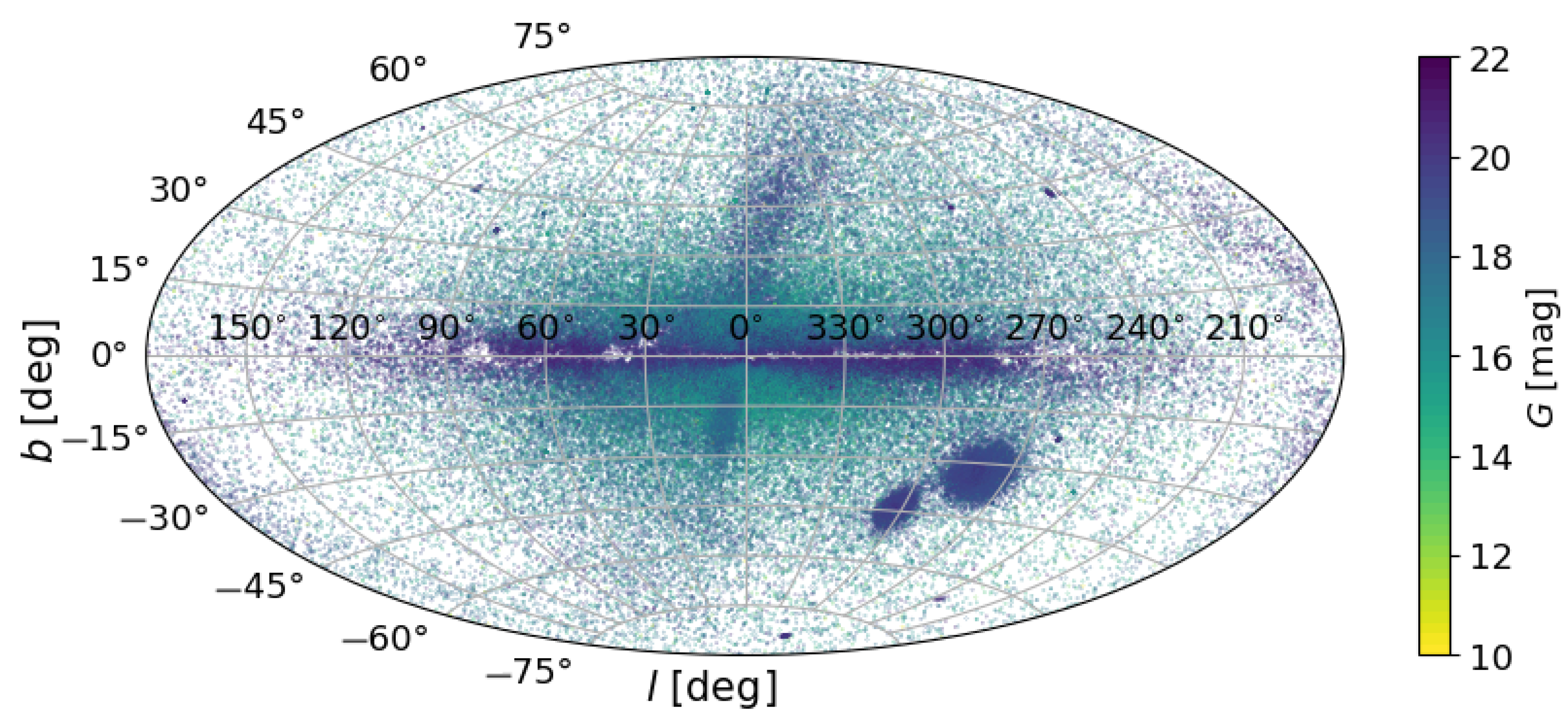
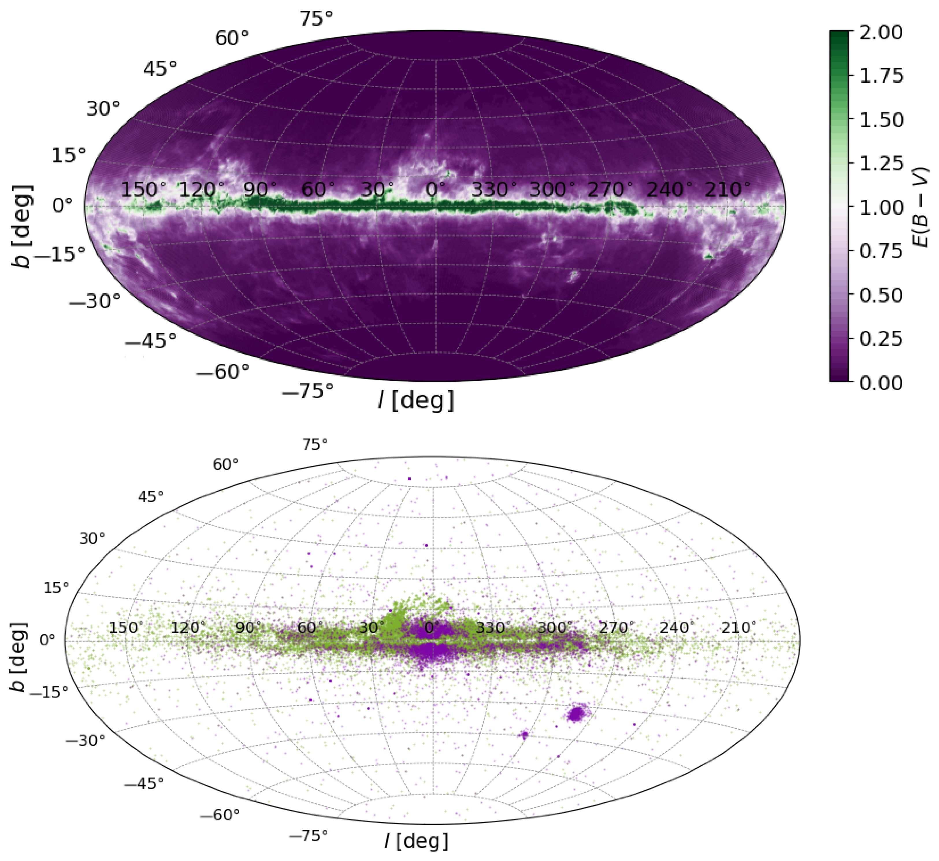
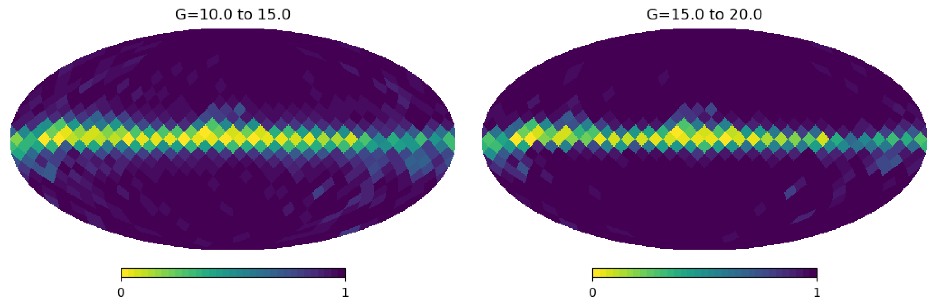
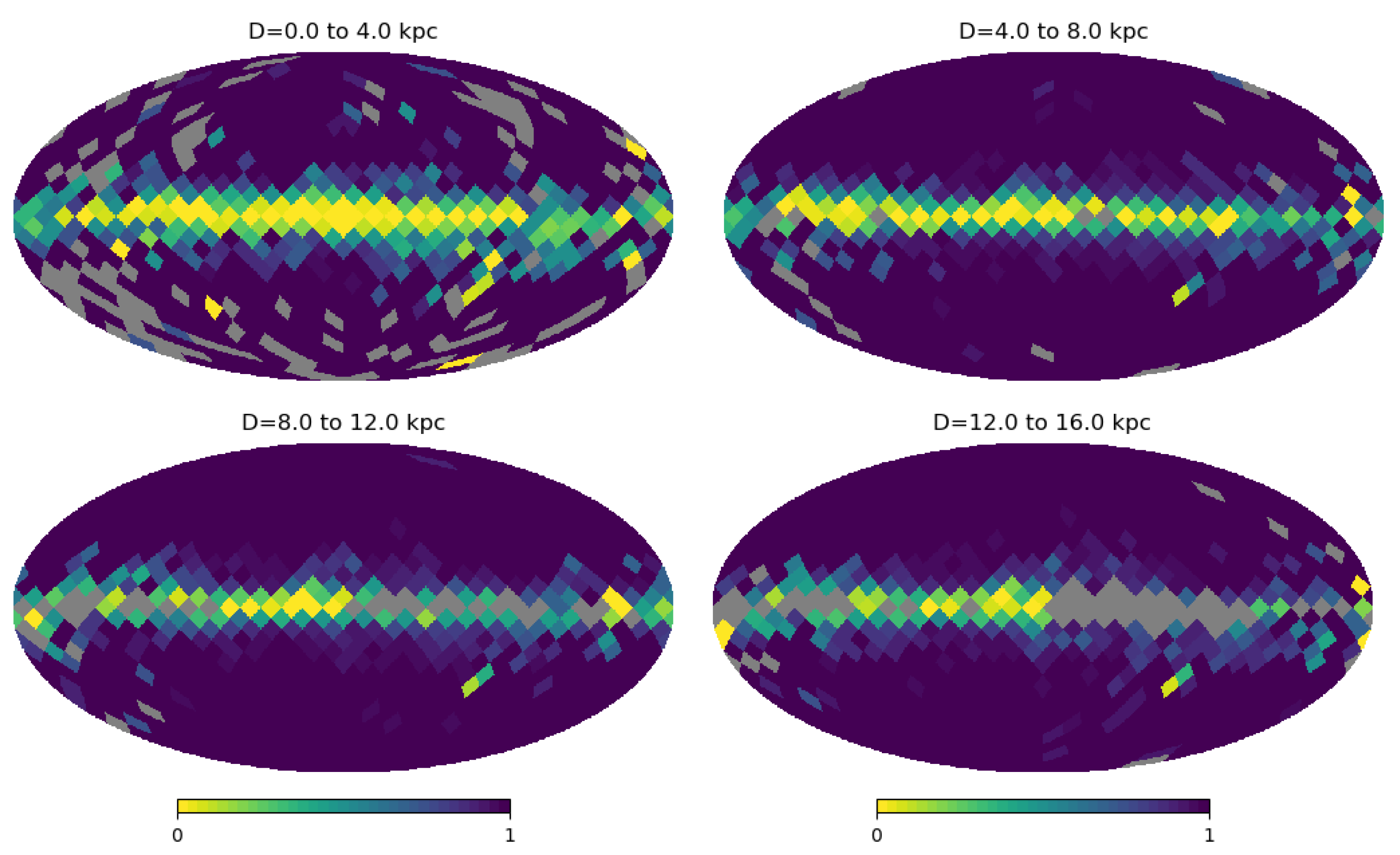
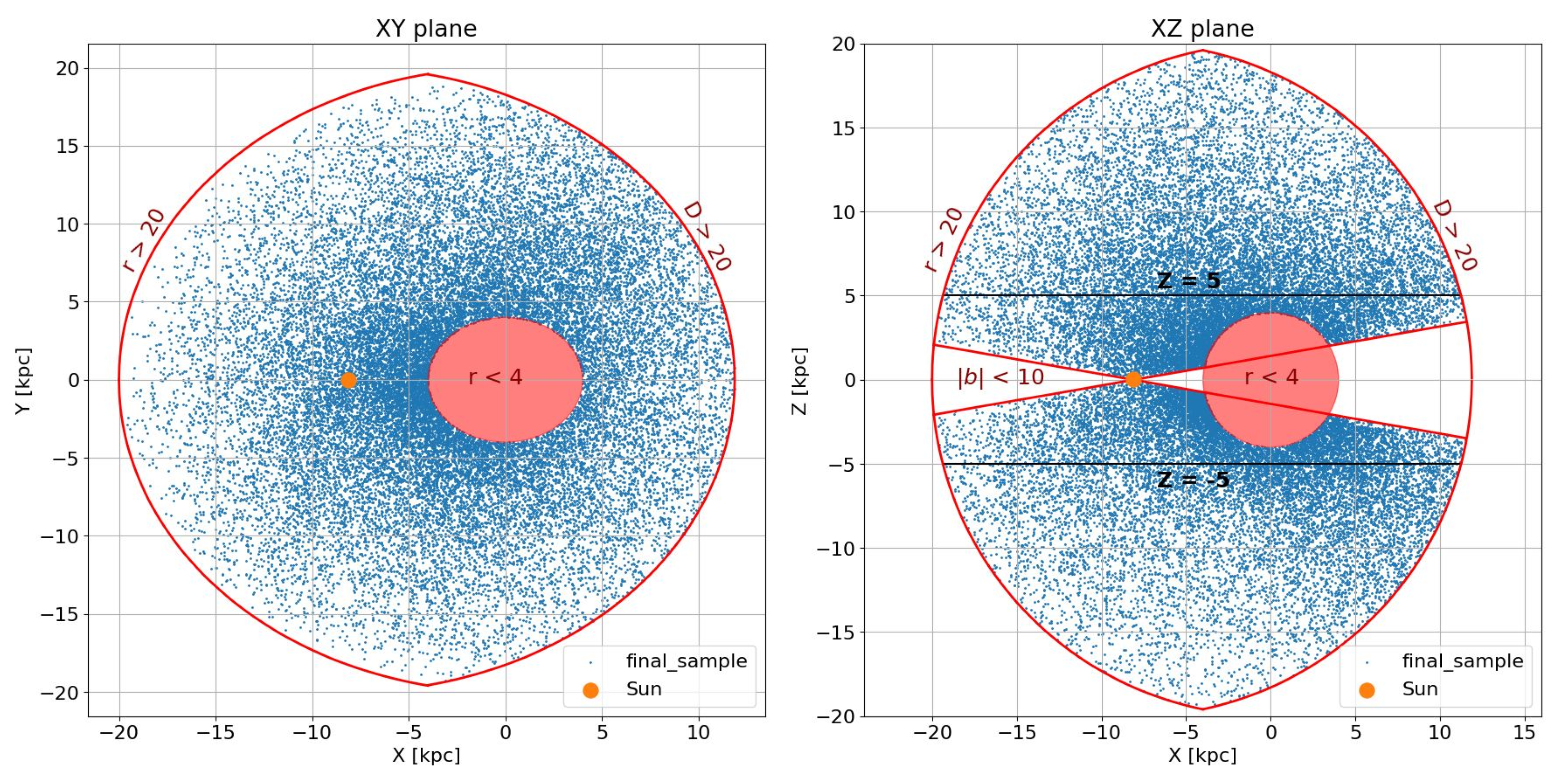
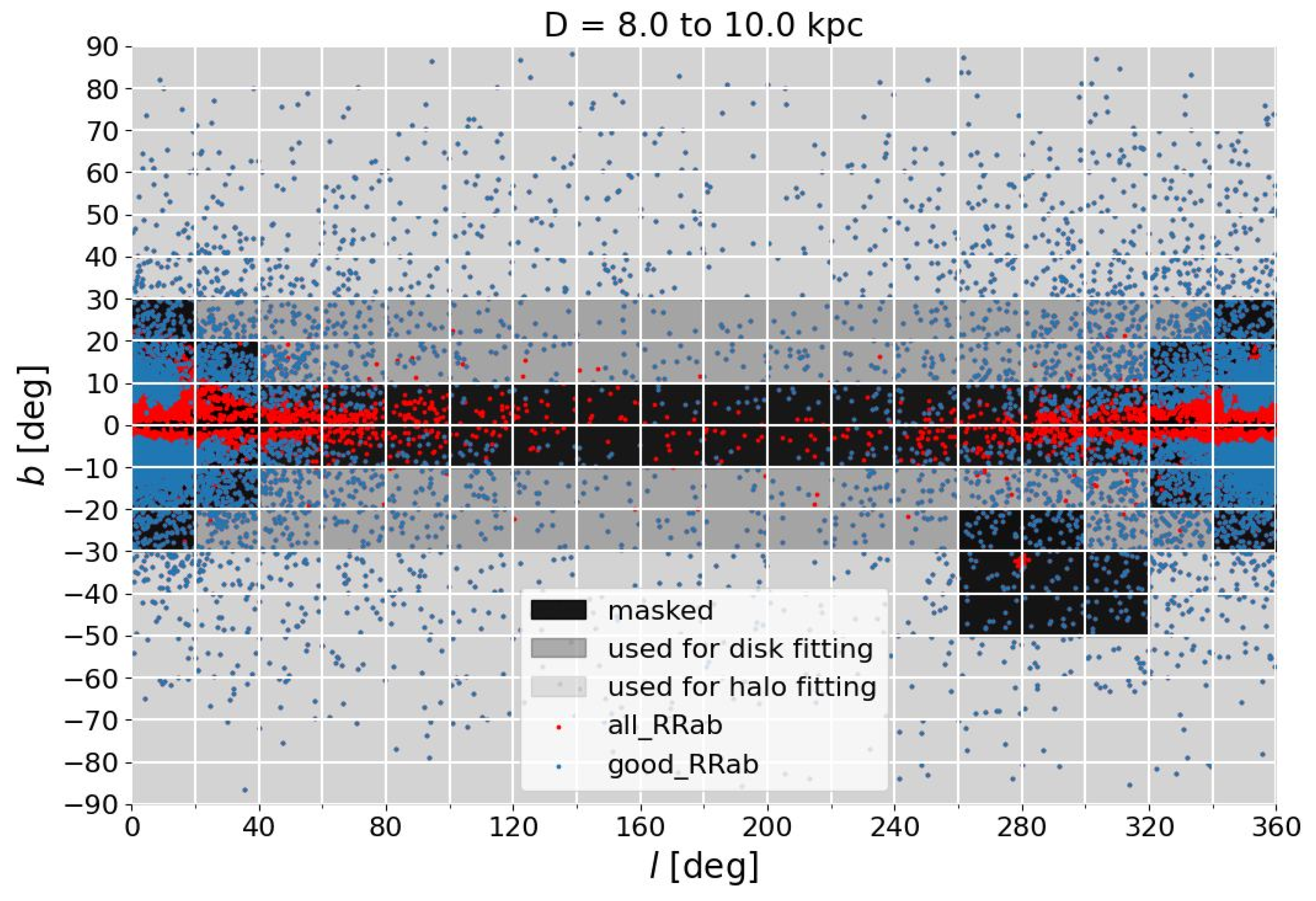
2.1. The Sample

We base our study on the publicly available catalog of RR Lyrae stars: the Gaia DR3 Specific Objects Study [16] (G < 20.7 mag), ASAS-SN-II [30] (G < 17 mag) and PanSTARRS1 [31] (G < 21 mag). From now on, we will refer to them as Gaia SOS, ASAS and PS1, respectively. Gaia SOS and ASAS are both all-sky, while PS1 covers about 3/4 of it. We cross-matched the Gaia SOS and ASAS with a 5″ tolerance, and Gaia SOS and PS1 with a 3″ tolerance parameter, as in Mateu et al. [32], Jayasinghe et al. [33]. Then, as in [14,32], we select only RRab type Lyrae stars and exclude RRc Lyraes because the latter have problems with completeness and contamination because the RRc contamination is significantly higher than the RRab. As a result, we have 175,350 RRab Lyraes from Gaia SOS,  61,829 stars from ASAS+PS1 combined and 53,424 cross-matched stars between the two samples, Gaia SOS and ASAS+PS1.

To convert the heliocentric coordinates into galactocentric ones, we use the astropy package [34,35,36], adopting the solar galactocentric distance $R_{\odot }=8.122$ kpc [37] and the vertical displacement of the Sun from the galactic plane $Z_{\odot }=20.8$ pc [38]. Figure 1 shows the sky distribution in galactic coordinates of the above uniquely selected 183,755 RRab Lyraes, which reflects the main structures reported in other studies: the Milky Way’s disc and halo, the Magellanic Clouds, and the Sagittarius Core and Stream.

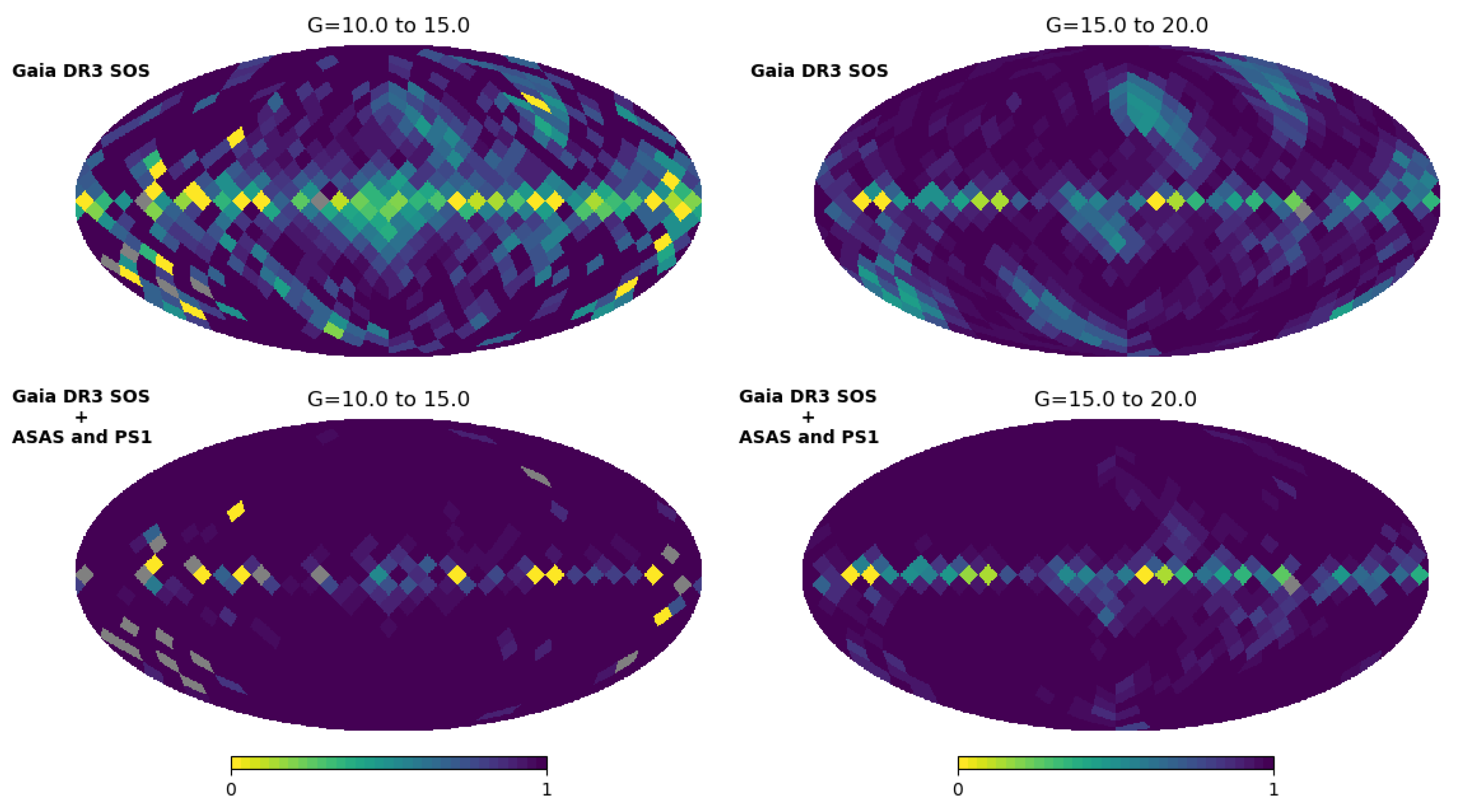
2.2. Selection Function

Constructing a selection function for a specific sample involves the usage of various criteria to measure or weight the selected sample of objects of interest against their whole true population. In other words, it aims to relate the observed number of objects $N_{obs}$ to the actual number of stars $N_{true}$ as $S=N_{obs}/N_{true}$. We define the selection function as a product of the two catalogs:

$$\begin{array}{c}\hfill S=S_{combined}{S}_{flag}.\end{array}$$

(1)

For the first function $S_{combined}$, we use a procedure suggested by Rybizki and Drimmel [39] for two independent catalogs and recently used in other studies [32,40,41]. We choose Gaia SOS as the first catalog and ASAS+PS1 as the second one. The probability that a given RRL is selected in the combined catalog, Gaia+(ASAS+PS1), is the sum of the individual probabilities minus the probability that it is present in both. Then, the selection function of the combined catalogs can be written as follows:

$$\begin{array}{cc}\hfill S_{\mathrm{combined}}=& S_{\mathrm{Gaia}}+S_{\mathrm{ASAS}+\mathrm{PS}1}\hfill \\ \hfill & -S_{\mathrm{Gaia}}\times S_{\mathrm{ASAS}+\mathrm{PS}1}.\hfill \end{array}$$

(2)

The completeness $S_A$ of the catalog A can be considered as the probability of detecting a star in this catalog—that is, the ratio of the number of the observed stars in the survey $N_A$ divided by the true number of stars $N_{\mathrm{true}}$:

$$\begin{array}{c}\hfill S_A=P_A={\displaystyle \frac{N_A}{N_{\mathrm{true}}}}.\end{array}$$

(3)

Assuming that the two catalogs are independent, we can write the number $N_{A\cap B}$ of the stars common to two catalogs as follows:

$$N_{A\cap B}=P_{A\cap B}{N}_{\mathrm{true}}=P_A{P}_B{N}_{\mathrm{true}}={\displaystyle \frac{N_A}{N_{\mathrm{true}}}}{\displaystyle \frac{N_B}{N_{\mathrm{true}}}}{N}_{\mathrm{true}}=S_A{N}_B⟹S_A={\displaystyle \frac{N_{A\cap B}}{N_B}}.$$

(4)

Similarly, for catalog B, ${\displaystyle S_B=\frac{N_{A\cap B}}{N_A}}$. It is also immediately apparent from Equation (4) that $S_{A\cap B}=S_A{S}_B$. In other words, by mutual comparison of each independent catalog with their intersection, we can assess their individual completeness. This procedure relies significantly on two assumed facts: no contamination in each catalog, and no mismatches between them. This procedure is employed to compute the completeness of ASAS and PS1 individually, of their combination (ASAS+PS1), of Gaia SOS and of their full combination (Gaia SOS+ASAS+PS1).

Figure 2 demonstrates the relative completeness of Gaia SOS (top row) and the completeness of the combined Gaia SOS+ASAS+PS1 catalog (bottom row) for two different intervals of apparent G magnitude. In this figure, we used the healpy Python software [42,43] and split the sky into HEALPix regions of level 3, corresponding to approximately $7.4$ deg² in galactic coordinates. As can be seen from the top row of Figure 2, there are patches of incompleteness in Gaia SOS which can be connected to the Gaia satellite scanning law.

We then apply the second selection function, which discards stars with bad quality measurements according to several criteria. As shown in previous works [16,44,45], the bad quality measurements are related to the crowded areas (galactic plane or bulge region) with a significant number of artifacts and spurious contaminants [46]. Following Cabrera Garcia et al. [17], we consider the values of ruwe and phot_bp_rp_excess_factor, which are applied to Gaia SOS, and $E(B-V)$, which is applied to both the Gaia SOS and ASAS+PS1 catalogs:

• ruwe$>1.4$.
• phot_bp_rp_excess_factor$>1.5$
• $E(B-V)>0.8$

The above conditions characterize the stars that will be rejected. The criterion imposed on ruwe (renormalized unit weight error) chooses sources whose astrometric solutions correspond well to a single-star five-parameter solution [47] and excludes blended sources or unresolved stellar binaries [48]. The phot_bp_rp_excess_factor gives the ratio between the combined flux in the Gaia $BP$ and $RP$ bands and the flux in the G band. Large values of this ratio are caused by blended sources [49]. The third criterion, reddening $E(B-V)$, is applied to both Gaia SOS and ASAS+PS1 catalogs.

Figure 3 shows the reddening map (top figure) taken from Schlegel et al. [50] with 14% correction taken from [51,52]. The bottom figure shows the distribution of the stars with a “bad” ruwe (purple points) and large BP/RP excess factor (green points). As can be seen from Figure 3, stars with bad quality measurements are concentrated near the galactic plane, in the regions with high concentration of dust and blended sources. When determining the parameters of the galactic thick disc and halo, we will exclude from consideration the areas of the sky with latitudes $\left|b\right|<{10}^{\circ }$.

Let us introduce the selection function $S_{flag}$, which is connected to the quality cut, as follows:

$$\begin{array}{c}\hfill S_{flag}=N_{Good}/N_{Total}.\end{array}$$

(5)

where $N_{Total}$ is the total number of stars and $N_{Good}$ is the number of stars not rejected by the three above-mentioned quality conditions. It should be noticed that if we have a star with a large ruwe or BP/RP excess factor in Gaia SOS but it is a reliable source in the ASAS+PS1 catalog, we select it as “good” and it is included in the $N_{Good}$ sample. We consider a star in ASAS+PS1 as reliable, following [32,40]1. In the ASAS catalog, RRLs with periods $<0.95$ d were discarded (to avoid the excess of spuriously identified stars) as well as those with suspiciously large amplitudes > 2 mag [32]. In the PS1 catalog, ‘bona fide’ sources have a classification score $scor{e}_{3,ab}>0.8$, which, according to [31], yields a sample with 0.97 purity and 0.92 completeness [32].

Figure 4 shows the completeness maps of the selection function $S_{flag}$ for two ranges of apparent G magnitude. In the areas close to the disc plane, completeness decreases to almost zero values, while outside the midplane of the disc it is close to $0.9$–1 (or  90–$100\%$).

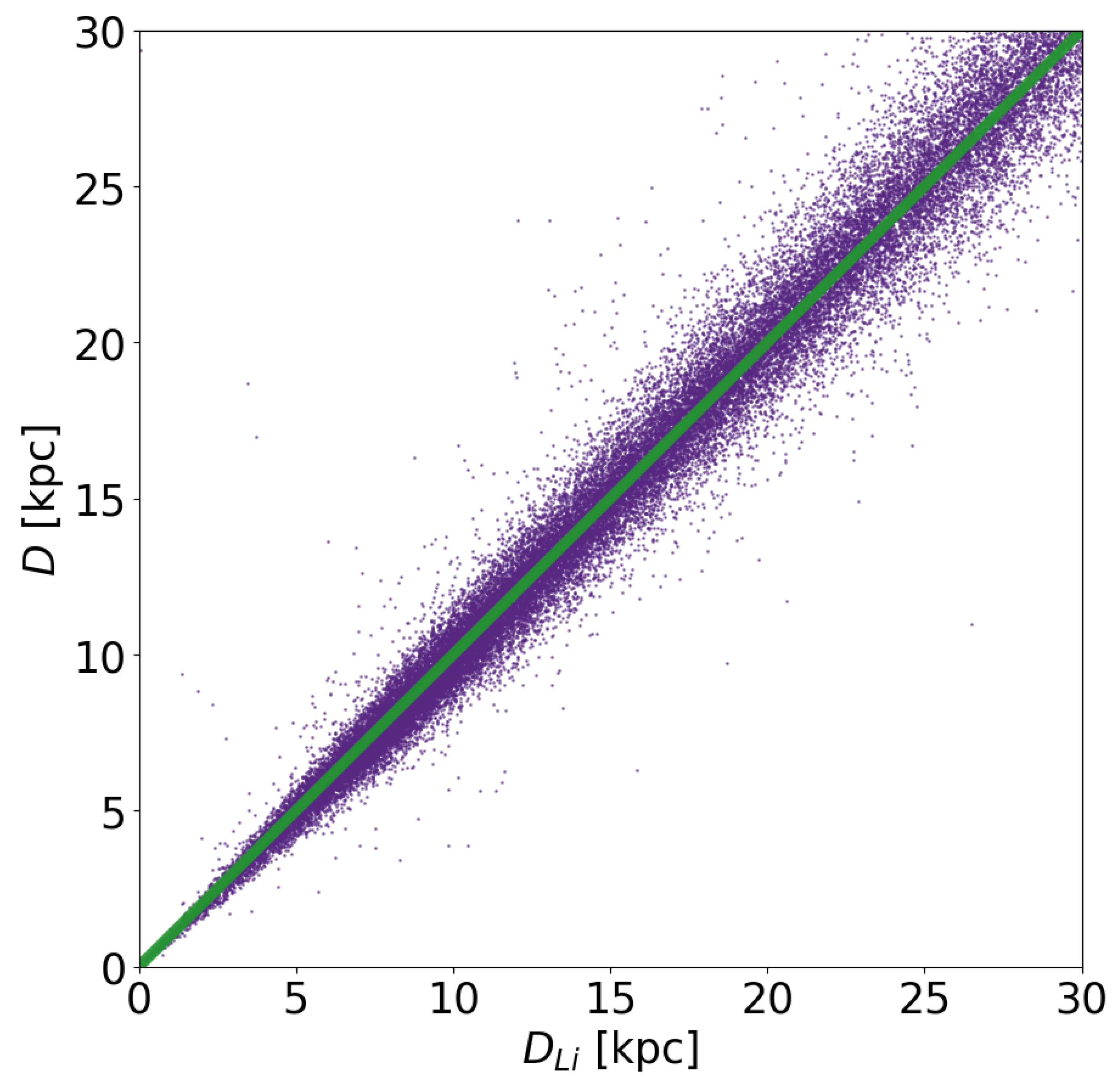
2.3. Distance Estimation

To determine the scale length and the scale height of the thick disc, we need to know a selection function not as a function of apparent G magnitude but as a function of distance. Only a fraction of stars (115,410 out of 183,755) have distances determined by Li et al. [53]. For the stars lacking distances, we calculate them using the following equation:

$$G=M_G+A_G+5{log}_{10}\left(D\right)-5.$$

(6)

where G is the apparent magnitude of the star in the Gaia G-band, $M_G$ is its absolute magnitude, D is its distance in parsecs, and $A_G$ is its extinction value. We take $M_G=0.6$, a mean value determined by [32,53], as the absolute stellar magnitudes for RRab Lyrae stars. Following [53], for stars with $\left|b\right|>{25}^{\circ }$, extinction was calculated using the expression from $A_G=R_{G}E(B-V)$, where $R_G=2.516$ [54], and $E(B-V)$ taken from the reddening maps from [50], taking into account the 14% systematic correction according to [51,52]. For the stars with latitudes $\left|b\right|\le {25}^{\circ }$, we take the extinction $A_G$ from [16]. For the sample of stars with accurately determined distances from Li et al. [53], Figure 5 compares them with our estimated distances computed using Equation (6), showing good agreement.

To obtain the selection function S from Equation (1) as a function of distance, we compute the aforementioned completeness for each HEALpix and a certain distance interval. Figure 6 plots the final selection function S for four distance ranges.

The next step in cleaning the sample is to eliminate regions related to globular clusters (GCs) and dwarf galaxies (DGs). To eliminate GC RRLs, we remove all the stars within a 10 half-light radius of each globular cluster listed in the Harris [55] catalog of GCs. Following Cabrera Garcia et al. [17], we exclude RRLs belonging to the Sagittarius Stream and Sagittarius Core by cross-matching their Gaia DR3 source_id with the catalog of Ramos et al. [56], and the DGs were deleted using Table C.2 of Gaia Collaboration et al. [57]. We also removed all RRLs towards the Magellanic Clouds within a diameter of ${16}^{\circ }$ and ${12}^{\circ }$ for Large and Small Clouds, respectively [17]. As mentioned above, we exclude the area with latitude of |b| < ${10}^{\circ }$ to avoid regions with a high content of dust and contaminations. We also excluded RRLs with a distance of $D>20$ kpc from our consideration.

After all of the above data cleaning (quality and spatial cuts), our observational sample consists of 40,188 unique RRLs. Of this final sample, 36,685 are listed in Gaia SOS and 33,703 in ASAS+PS1. There are 30,200 RRLs in common between both catalogs; 2982 RRLs are only in Gaia SOS, and reciprocally, 3503 are listed only in ASAS+PS1. We have 31,978 out of 40,188 RRLs with accurate distances from Li et al. [53] and 8210 (20%) with distances estimated by us.

3. Thick Disc and Halo Fitting Model

3.1. Density Profile Models

We assume that the density profile of the selected RRLs can be described in galactocentric cylindrical coordinates $(R,z)$ as a sum of the halo and thick disc distributions, assuming the absence or a negligible amount of thin disc RRLs (Minniti et al. [58] have shown the absence of metal-rich RRLs, which can be associated with the thin disc [14]) in the Milky Way:

$$C(R,z)=C_{disc}(R,z)+C_{Halo}(R,z).$$

(7)

3.1.1. The Thick Disc

To model the thick disc density profile, we use two types of density distribution. In the first one, we use the standard double exponential density profile [10,14]:

$$C_{Disc}(R,z)=C_{Disc,\odot }{e}^{-\frac{R-R_{\odot }}{h_R}}{e}^{-\frac{\left|z\right|}{h_z}}.$$

(8)

where $h_z$, $h_R$ and $C_{Disc,\odot }$ are the vertical scale height, the radial scale length and the concentration of RRLs in the solar neighborhood, respectively. $R_{\odot }$ is the distance of the Sun from the galactic center, taken to be 8.122 kpc. In the second case, for the vertical density distribution of the thick disc, we assume the profile $sec{h}^2$ [2,10,59]:

$$C_{Disc}(R,z)=C_{Disc,\odot }{e}^{-\frac{R-R_{\odot }}{h_R}}sec{h}^2(-z/h_z),$$

(9)

where $h_z$, $h_R$ and $C_{\odot }$ are the same values as in Equation (8). We do not consider the thick disc flare in our study because the thick disc is flat in the inner regions with radii of $R<14$–16 kpc [9,60].

3.1.2. The Halo

For the halo density distribution, we use the standard power law [14]:

$$C_{Halo}(R,z)=C_{Halo,\odot }{\left[R^2+{\left({\displaystyle \frac{z}{q}}\right)}^2\right]}^{n/2},$$

(10)

where $C_{Halo,\odot }=C_{Halo}/R_{\odot }^n$ is the halo RRL concentration in the solar vicinity, and q is the halo flattening.

From the kinematic parameters of stars from SDSS, Carollo et al. [61] suggested a dual halo model for the Milky Way galaxy, where the inner halo is dominated by the radial merger of some massive metal-rich clumps, while the outer halo consists of dissipation-less chaotic merging of smaller subsystems [62]. Different breaking spherical radii ranging from 20 to 30 kpc [25,46,61,62] are proposed in articles where the parameter n may vary due to the two-component halo. Since we are aiming to estimate the scale length and scale height of the thick disc, it is reasonable to limit ourselves to the inner halo with spherical radii of $r<20$ kpc. Excluding the region with $r<4$ kpc is necessary to avoid contamination from the bar/bulge subsystems (the bar extends up to ∼5 kpc, where its scale height is ∼$0.180$ kpc [63]).

3.2. Fitting Procedure

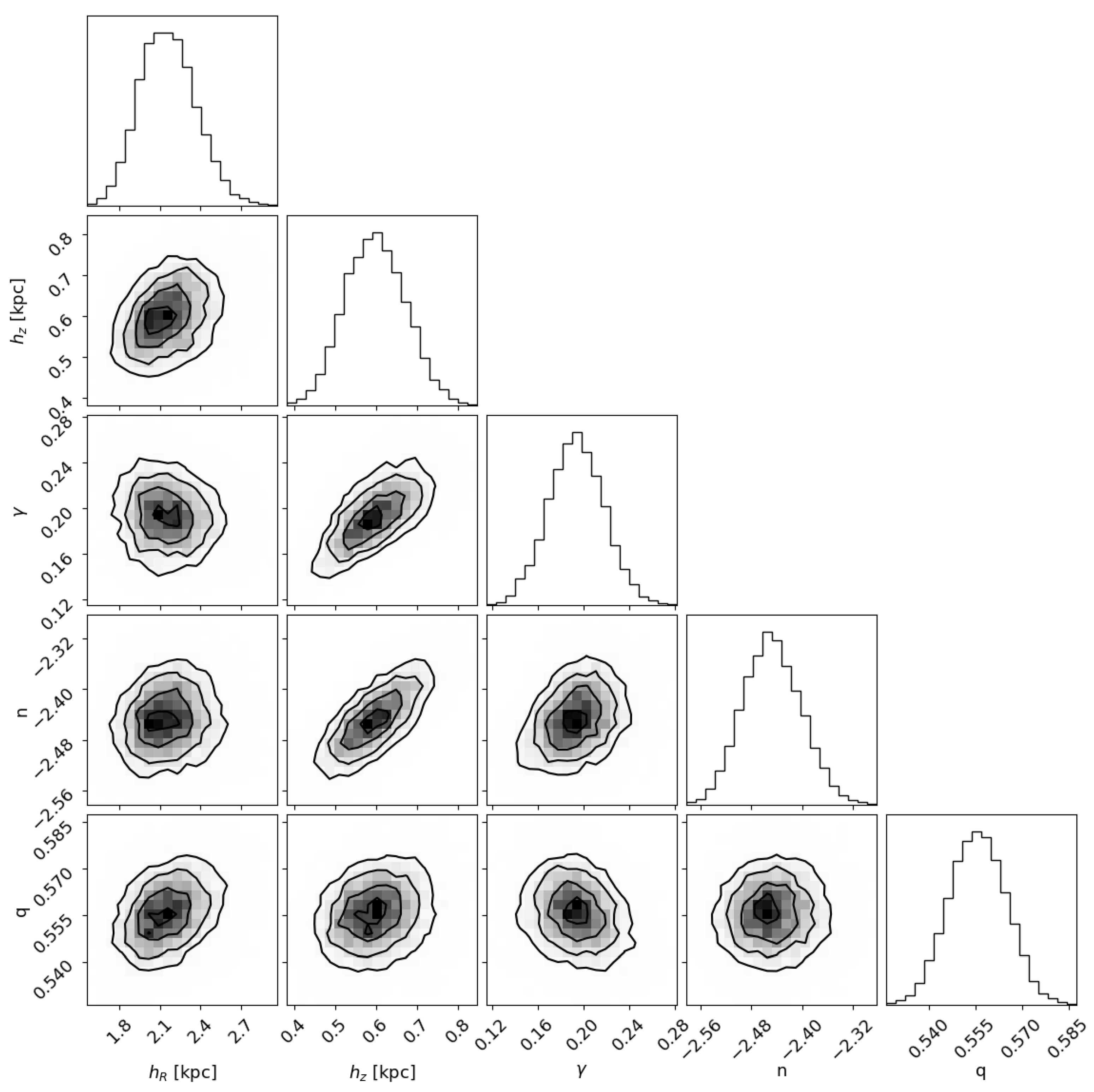
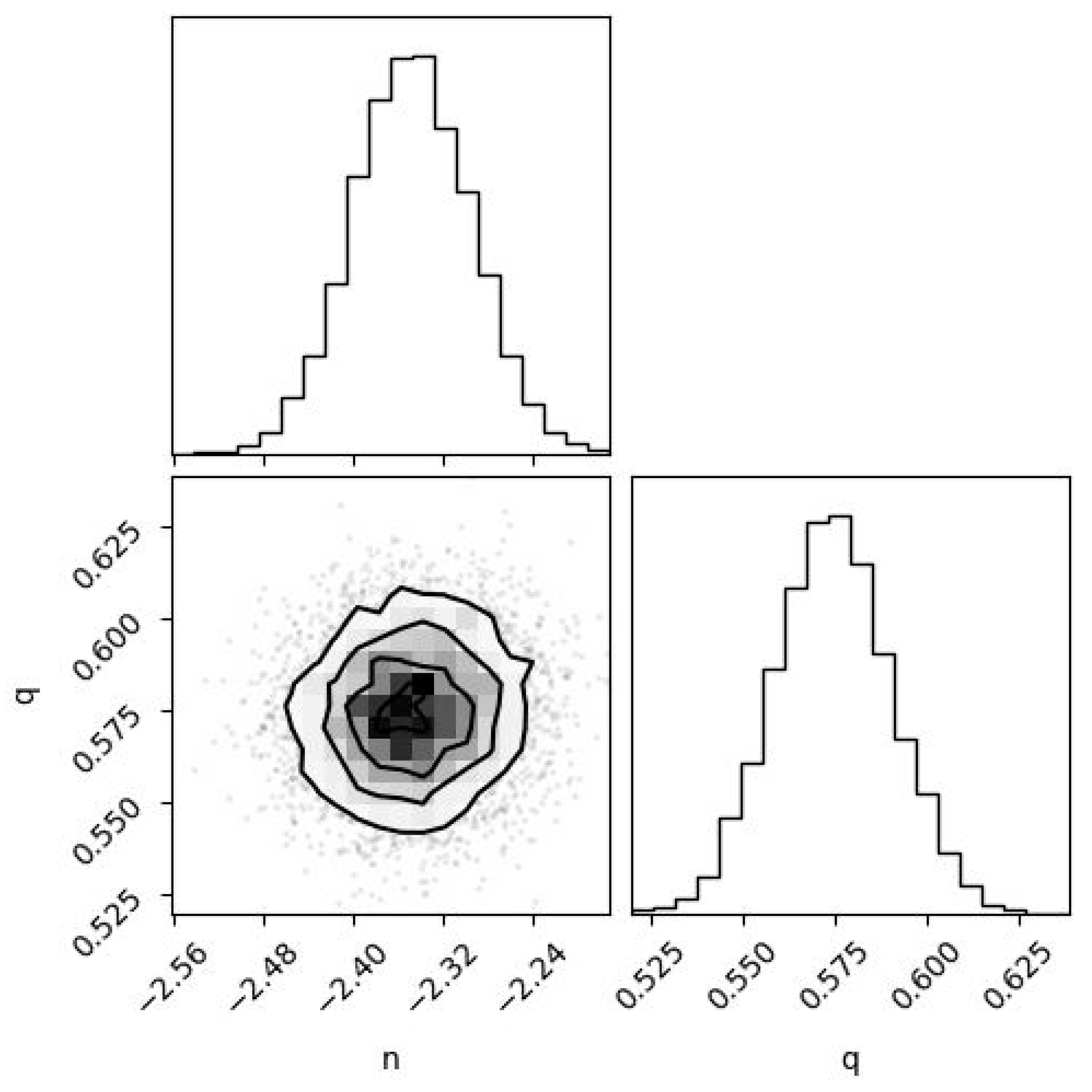
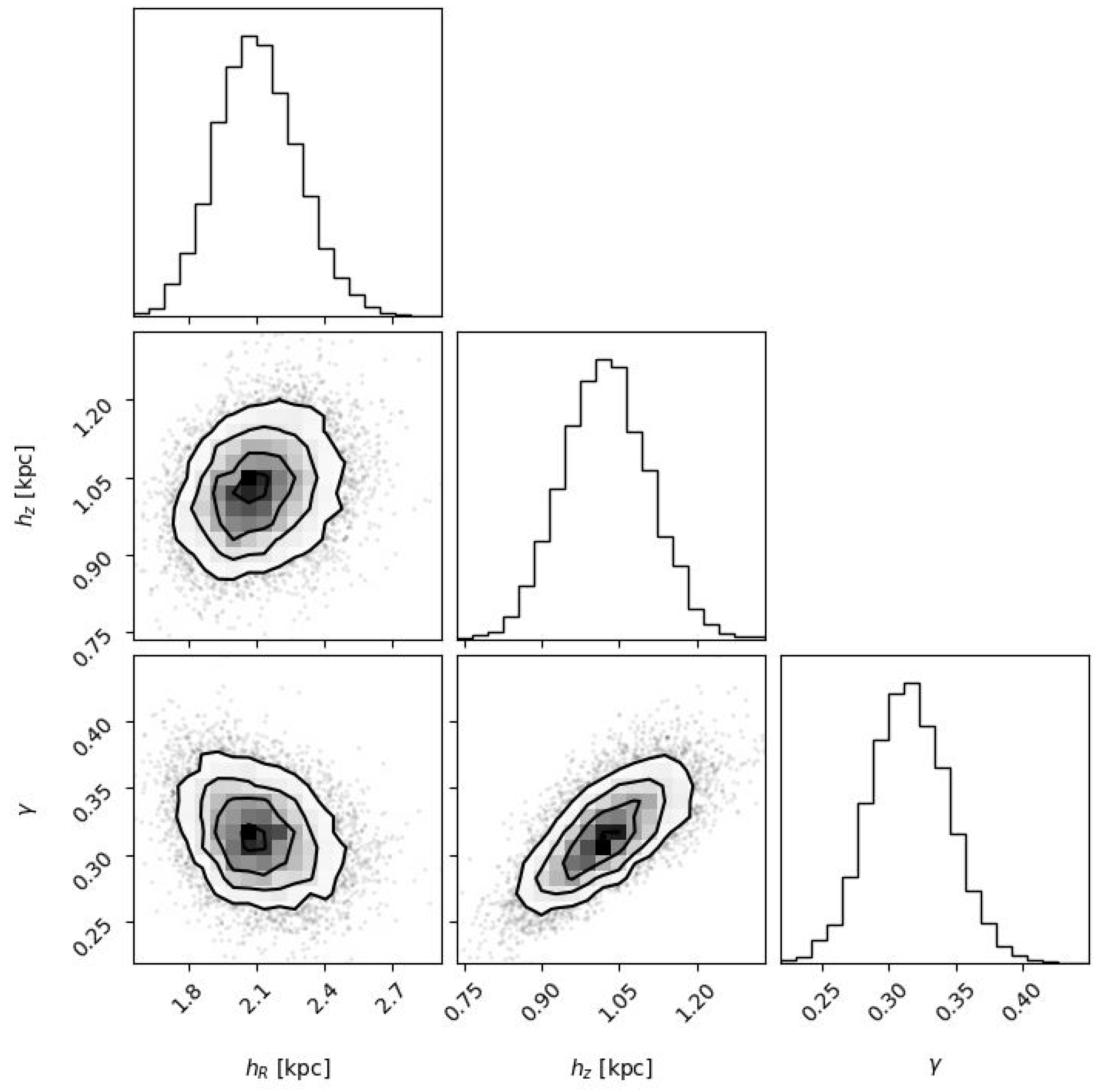
The fitting task is performed in two parts. First, we fit just the halo and find the parameters n and q (two free parameters fitting). For this part, we restrict the sampled volume by $\left|z\right|>5$ kpc and $4<r<20$ kpc to avoid the outer halo, disc and central bulge/bar, and we assume that the disc concentration $C_{disc}(R,z)$ in Equation (7) is zero. The number of stars in the experiment is 10,404.

After that, we keep the parameters of the halo fixed and adjust the parameters of the thick disc $h_z$, $h_R$ and the ratio of the concentration of halo stars to the concentration of the thick disc $\gamma =C_{Halo,\odot }(R,z)/C_{Disc,\odot }(R,z)$ in the solar neighborhood (three free parameters fitting). When fitting the thick disc, we restrict our region by a cylindrical radius of $4<R<20$ kpc and a height of $\left|z\right|<5$ kpc. The number of stars in the experiment is 11,707.

Figure 7 demonstrates distribution of our final RRL sample in the $(x,y)$ and $(x,z)$ plane, marking the areas where the fitting is performed. The galactic center is located at $x=0$ kpc and $y=0$ kpc.

We use the following procedure: We split our galaxy into custom bins in the galactic coordinates $(l,b,D)$ with sizes of ${20}^{\circ }$, ${10}^{\circ }$ and 2 kpc, respectively, and find the number of RRLs in each bin i according to Equation (7) as follows:

$$N_i={\int }_{V_i}C(l,b,D)dV={\int }_{l_i}^{l_{i+1}}{\int }_{b_i}^{b_{i+1}}{\int }_{D_i}^{D_{i+1}}C·cos\left(b\right)·D^{2}dl·db·dD,$$

(11)

where $C(l,b,d)$ is the number density as a function of the galactic coordinates. The HEALPixes are constructed as equal area pixels, which implies that there are certain levels of grid resolution. Since we integrate the density function within the bin, we are not forced to use equal area bins; therefore, we use our custom bins with more suitable sizes for our sample. We use masks to remove the bins that contain Magellanic Clouds. We remove stars in the direction of globular clusters and dwarf galaxies, as described above; however, we do not mask the corresponding bins because the spatial size of the removed area is significantly smaller compared to the bin size (<1 percent of the bin area for all clusters and dwarf galaxies). Figure 8 demonstrates our custom bins in the galactic coordinates for the slice of radii from 8 to 10 kpc with blue points (‘good’ stars) and red points (‘bad’ stars). Bins with black backgrounds describe masked bins, which are not used in the fitting. The grey and dark grey colors mark the area where the halo and the thick disc are fitted.

Then, to find the selected number of RRLs in each bin, we multiply by the value of the selection function from Equation (1):

$$N_{selected,i}=N_i·S_i$$

(12)

Then, we construct the probability density function of the RRLs to be observed from the selected number of RRLs by normalizing the sum to 1. Finally, we derive the number of RRLs generated in each bin as a probability density function multiplied by the total number of observed RRLs. In other words, we distribute the total number of observed RRLs among the bins according to the probability density function:

$$N_{gen,i}={\displaystyle \frac{N_{selected,i}}{{\sum }_{i=1}^M{N}_{selected,i}}}·\sum _{i=1}^M{N}_{obs,i}$$

(13)

where M is the total number of bins.

We estimate the parameters of the models through Bayes inference using the procedure from Tremmel et al. [64]. We assume that the observed number of RRLs ($m_i$) in our bins is drawn from an underlying Poisson distribution

$$p\left(m_i\right|{\lambda }_i)={\displaystyle \frac{e^{-{\lambda }_i}{\lambda }_i^{m_i}}{m_i!}}$$

(14)

where we are not interested in the Poisson mean $\lambda$, so we marginalize over it.

$$p\left(m\right|\theta )=\prod _i\int p\left(m_i\right|{\lambda }_i)p\left({\lambda }_i\right|\theta )d{\lambda }_i$$

(15)

where $\theta$ is the set of parameters used for fitting.

Assuming that the generated number of RRLs ($n_i$) is distributed with the same Poisson distribution

$$p\left(n_i\right|{\lambda }_i)={\displaystyle \frac{e^{-{\lambda }_i}{\lambda }_i^{n_i}}{n_i!}},$$

(16)

we can estimate $p\left({\lambda }_i\right|\theta )$ by applying Bayes’ rule

$$p\left({\lambda }_i\right|\theta )=p\left({\lambda }_i\right|n_i\left(\theta \right))={\displaystyle \frac{p\left(n_i\right|{\lambda }_i)p\left({\lambda }_i\right)}{p\left(n_i\right)}},$$

(17)

where $\theta$—model parameters. Using Jeffreys prior on ${\lambda }_i$: ${\displaystyle p\left({\lambda }_i\right)=\frac{1}{\sqrt{{\lambda }_i}}}$, we obtain

$$p\left({\lambda }_i\right|\theta )={\displaystyle \frac{e^{-{\lambda }_i}{\lambda }_i^{n_i-\frac{1}{2}}}{\mathsf{\Gamma }(n_i+\frac{1}{2})}}$$

(18)

Inserting Equations (14) and (18) into Equation (15), we obtain

$$p\left(m\right|\theta )=\prod _i{\displaystyle \frac{\mathsf{\Gamma }(m_i+n_i+\frac{1}{2})}{2^{m_i+n_i+\frac{1}{2}}\mathsf{\Gamma }(n_i+\frac{1}{2})m_i!}}$$

(19)

Taking the logarithm and simplifying

$$log\left(p\right)=\sum _i^M\left[log\mathsf{\Gamma }(m_i+n_i+{\displaystyle \frac{1}{2}})-log\mathsf{\Gamma }(n_i+{\displaystyle \frac{1}{2}})\right]-log2(M+N+{\displaystyle \frac{1}{2}})-\sum _i^{M}log{m}_i!$$

(20)

And then omitting the constants

$$log\left(p\right)\sim \sum _i^M\left[log\mathsf{\Gamma }(m_i+n_i+{\displaystyle \frac{1}{2}})-log\mathsf{\Gamma }(n_i+{\displaystyle \frac{1}{2}})\right]$$

(21)

Thus, when $m_i=n_i$, the likelihood $log\left(p\right)$ reaches its maximum. Using uniform priors for parameters, we find that the posterior is

$$p\left(\theta \right|m)={\displaystyle \frac{p\left(m\right|\theta \left)p\right(\theta )}{p\left(m\right)}}\propto p\left(m\right|\theta )$$

(22)

We used a Markov chain Monte Carlo (MCMC) method, specifically the sampler from the emcee [28] Python package, to explore the posterior PDF. We used 16 chains per parameter, performing 3000 steps in total. After convergence was reached (500 steps for the burn-in phase), we obtained the results.

As an additional test, we independently used the Nautilus [29] Python package, which uses the importance nested sampling (INS) technique for the Bayesian posterior, and found essentially identical results.

4. Results

All the best-fit parameter results in this study are presented as the median value and $\pm 1\sigma$ equivalent range, with the latter being defined by the 15.87 and 84.13 percentiles. In the first step of the fitting procedure, we determined the exponent of the halo power law density profile to be $n=-{2.35}_{-0.05}^{+0.05}$ and flattening $q={0.57}_{-0.02}^{+0.02}$.

Table 1. Best fitting parameters of the thick disc and halo.

Halo
	n	q
median±range	$-{2.35}_{-0.05}^{+0.05}$	${0.57}_{-0.02}^{+0.02}$
mean±1$\sigma$	$-{2.35}_{-0.05}^{+0.05}$	${0.57}_{-0.02}^{+0.02}$
Thick disc with exponential vertical profile
	$h_R$	$h_z$	$\gamma$
median±range	$-{2.14}_{-0.17}^{+0.19}$ kpc	${0.64}_{-0.06}^{+0.06}$ kpc	${0.19}_{-0.02}^{+0.02}$
mean±1$\sigma$	$-{2.14}_{-0.18}^{+0.18}$ kpc	${0.64}_{-0.06}^{+0.06}$ kpc	${0.19}_{-0.02}^{+0.02}$
Thick disc with ${\mathit{sech}}^2$ vertical profile
	$h_R$	$h_z$	$\gamma$
median±range	$-{2.10}_{-0.17}^{+0.19}$ kpc	${1.02}_{-0.08}^{+0.09}$ kpc	${0.32}_{-0.03}^{+0.03}$
mean±1$\sigma$	$-{2.11}_{-0.18}^{+0.18}$ kpc	${1.02}_{-0.08}^{+0.08}$ kpc	${0.32}_{-0.03}^{+0.03}$

The halo power law density exponent n and flattening q, the thick disc scale length $h_R$ and height $h_z$, and the halo to disc concentration ratio $\gamma$ obtained in this work.

shows the obtained results and also includes the mean values and standard deviations. In Figure 9, we show the corresponding ‘corner plot’, i.e., the density plot of the two-dimensional projections of the PDF, showing the relationship between the parameters n and q. The black circular lines correspond to areas with $1\sigma ,2\sigma ,3\sigma$ equivalent ranges.

It is important to note that the resulting flattened inner halo of the RRLs should not be associated with the dark matter halo. The explanation of the stellar halo’s flatness is linked to the accretion history of the Milky Way and can be related, for example, to the dominant influence of the Gaia Sausage/Enceladus accretion at redshift $z\approx 2$ [65,66,67].

At the second step, with the halo parameters found above fixed, we fitted the parameters of the thick disc $h_z$, $h_R$ and the halo to the thick disc concentration ratio $\gamma =C_{Halo,\odot }(R,z)/C_{Disc,\odot }(R,z)$ in the solar neighbourhood for each of the two disc vertical profile models: exponential and $sec{h}^2$. For the exponential profile, we found $h_R={2.14}_{-0.17}^{+0.19}$ kpc, $h_z={0.64}_{-0.06}^{+0.06}$ kpc and $\gamma ={0.19}_{-0.02}^{+0.02}$. For the $sec{h}^2$ profile, we found $h_R={2.10}_{0.17}^{+0.19}$ kpc, $h_z={1.02}_{-0.08}^{+0.09}$ kpc and $\gamma ={0.32}_{-0.03}^{+0.03}$. Table 1 also shows the best-fit parameters of the thick disc and halo to disc concentration ratio for both vertical profile models. Figure 10 and Figure 11 show the corresponding corner plots. For both models, we obtain almost identical thick disc radial scales; however, the choice between the two vertical scale laws has a noticeable effect on determining the ratio of the halo to the disc concentration from $19\%$ to $32\%$ for the exponential and $sec{h}^2$ vertical profile, respectively.

We also performed the five-parameter fitting of the halo and thick disc simultaneously, limiting the analysis to the spherical radii of $4<r<20$ kpc. We obtained very similar results, with the vertical scale showing the greatest deviation in the case of the $sec{h}^2$ vertical profile, reaching a 10% difference. However, taking into account the errors, we obtained the same results with both approaches. These results can be found in Appendix A.

5. Discussion

The parameters of the thick disc are determined by the mechanism of its formation. A few scenarios for explanation of the origin of the thick disc have been suggested, which can be divided into three groups. The first type of scenario explains the origin of the thick disc by heating of the pre-existing thin disc. The first physical mechanism for such heating was suggested by Spitzer and Schwarzschild [68], who proposed that the scattering of thin disc stars by molecular clouds could produce the thick disc. Later, other mechanisms were proposed, including heating by spiral structure (Sellwood and Carlberg [69]), minor mergers with accreted small satellites [70], and radial migration of stars, as considered by Schönrich and Binney [71], as possible mechanisms for thick disc formation. Another approach to explain the origin of the Milky Way’s thick disc involves a major accretion of a satellite galaxy. Abadi et al. [72] suggests that the thick disc was formed from the stars born in a disrupted massive satellite galaxy. An “intermediate” scenario of thick disc formation assumes that gas-rich mergers trigger an episode of thick disc formation. Grand et al. [73] analyzed the Auriga cosmological zoomed-in Milky Way-like galaxy simulations and came to the conclusion that the formation of the thick disc was caused by a massive Gaia Sausage/Enceladus-like merger with a massive gas-rich satellite with a mass of ${10}^{8-9.5}$$M_{\odot }$, which caused a dual effect on the evolution of the Milky Way galaxy. It “splashed” the existing proto-disc stars into the halo, brought fresh gas into the central regions of the galaxy and triggered a starburst that formed a thick disc.

Park et al. [74] analyzed the results of high-resolution cosmological simulations in GALACTICA and NEWHORIZON to understand whether the spatially distinct thin and thick discs are formed by different mechanisms. These authors traced the birthplaces of the stellar particles in the thin and thick discs and found that most of the thick disc stars in simulated galaxies were formed close to the midplane of their discs, which suggests that the two discs are not distinct in terms of formation mechanism but rather are the signature of a complex formation of the Milky Way’s disc. This scenario is supported by the findings of Vieira et al. [75], who used RGB stars from the GAIA DR3 catalog and found that about half of the stars in the solar neighborhood have thick disc kinematics. Later, Vieira et al. [15] confirmed this result using a complete sample of about 330,000 dwarf stars which were well-measured by Gaia DR3, finding that the ratio of the concentration of the thick disc dwarf stars to the concentration of stars with thin disc kinematics in the solar neighborhood is 0.75 ± 0.05, which is consistent with the result based on the RGB-stars. Finding that the thick stellar disc is as massive as the thin one changes our understanding of thick disc formation. If the mass of the Milky Way’s thick disc is comparable to that of the thin one, i.e., in the order of 10¹⁰ solar masses, then an accreted gas-rich massive satellite galaxy should have a mass of about a few times 10¹⁰–10¹¹ solar masses. The accretion of such massive satellites will destroy a pre-existing disc, and the result of such accretion could lead to the formation of an elliptical galaxy. The formation of the thick disc looks rather like an evolutionary stage in the formation of the Milky Way’s multi-component and multi-structured thick disc. In light of this, we can understand the discrepancies in estimates of the radial scale length and the scale height of the thick disc based on the different objects mentioned above. It might be that the oldest thick disc objects, like RR Lyrae or BHB stars, trace the early stages of building the modern Milky Way’s thick disc, while the main sequence stars trace its later stages.

As mentioned in the introduction section, several attempts have been made to determine the parameters of the thick disc of the Milky Way. For example, using UBV color–magnitude diagram fitting, Robin et al. [8] found the galactic thick disc radial scale length and scale height to be $2.8\pm 0.8$ kpc and $0.76\pm 0.05$ kpc, respectively. Robin et al. [9], also using color–magnitude diagram (CMD) fitting, found those values to be $2.3$ kpc and $0.47$ kpc, respectively, for the $sec{h}^2$ vertical profile. Using the photometric parallax for 48 million stars detected by the Sloan Digital Sky Survey (SDSS), Jurić et al. [10] determined values of $h_R=2.6$ kpc and $h_z=0.9$ (for the exponential profile) kpc, respectively, for the thick disc. Bensby et al. [3], using K-giant stars, determined the thick scale length to be $2.0$ kpc. Bovy et al. [76], using G-dwarfs from SDSS, determined the thick disc $h_R$ and $h_z$ to be $2.01$ kpc and $0.686$ kpc (for the exponential profile), respectively. Recently, Vieira et al. [15], using a complete sample of about 330,000 dwarf stars that were well-measured by Gaia DR3, found the thick disc scale height to be $0.797\pm 0.012$ kpc for the $sec{h}^2$ vertical profile. Mateu and Vivas [14] listed in Table 6 the scale height and the scale length of the thick disc obtained by different authors. As one can see from this Table, the radial scale length determinations vary from 1.9 ± 0.1 [77] to 4.7 ± 0.2 [12]. The determinations of the vertical scale height of the thick disc vary from 0.51 ± 0.04 [13] to 1.06 ± 0.05 [78].

Using a combination of public RR Lyrae star catalogs totaling 1305 stars and Bayesian fitting, Mateu and Vivas [14] found $h_R=2.1$ kpc and $h_z=0.65$ kpc (for the exponential profile), respectively, using an exponential vertical profile law. Our results of $h_R={2.14}_{-0.17}^{+0.19}$ kpc and $h_z=0.64\pm 0.06$ kpc for the same profile coincide very well with these findings. As for the halo parameters, Mateu and Vivas [14] determined $n=-{2.78}_{-0.05}^{+0.05}$ and $q={0.9}_{-0.03}^{+0.05}$, which are different from ours. Finally, their halo to disc concentration ratio was estimated to be 23–$27\%$, while our results extend over a slightly larger range, from 19–32%. It is worth noting that our RRL sample is ∼20 times larger than theirs.

Other investigations of the Milky Way’s halo have relied, in many cases, on RRLs. For example, Sesar et al. [23] found $n=-2.42$ and $q=0.63$ using RRLs, which are close to our values. Similarly, Sesar et al. [24] found $n=-2.62\pm 0.04$ and $q=0.7\pm 0.02$. Recently, Iorio and Belokurov [79], using a Gaia DR3 RRL sample, found a significant flattening in the Milky Way’s stellar halo, with $0.5\lesssim q\lesssim 0.8$. Finally, using the photometric parallax for 48 million stars in SDSS, Jurić et al. [10] determined the values $n=-2.8\pm 0.2$ and $q=0.64\pm 0.1$. Our result of $n=-2.35\pm 0.05$ is slightly higher and indicates flattening, which is consistent with their numbers. In general, the parameters n and q vary widely in the literature, with $-3.75\lesssim n\lesssim -2.3$ and $0.5\lesssim q\lesssim 1$ [10,14,23,24,79,80,81].

Overall, our investigation and results stand out for having used a very large sample (+20,000 stars) of high-quality (RRLs) data, giving robustness to the estimated parameters.

6. Conclusions

Our study of the galactic thick disc and internal stellar halo has provided insights into their density distributions by using the most complete sample available of RRLs built from the Gaia DR3 SOS, ASAS-SN-II and PanSTARRS1 catalogs.

We applied Bayesian methods to find the thick disc scale length and height as well as the halo parameters of the Milky Way. We used an MCMC approach to determine these parameters and their statistical uncertainties. We also employed the INS technique for the Bayesian posterior and found essentially identical results.

We have determined the exponent of power law density profile of the halo to be $n=-{2.35}_{-0.05}^{+0.05}$ with flattening of $q={0.57}_{-0.02}^{+0.02}$. The thick disc scale length is $h_R={2.14}_{-0.17}^{+0.19}$ kpc, the scale height is $h_z={0.64}_{-0.06}^{+0.06}$ kpc and the concentration ratio (halo to disc) is $\gamma ={0.19}_{-0.02}^{+0.02}$ for the $sec{h}^2$ vertical profile. For the exponential vertical profile, the values are $h_R={2.10}_{0.22}^{+0.19}$ kpc, $h_z={1.02}_{-0.08}^{+0.09}$ kpc and $\gamma ={0.32}_{-0.03}^{+0.03}$.

Further progress in parameter refinement may be made with future Gaia releases, as well as progress in measuring the metallicities of RRLs and their radial velocities, which would provide complete 6D phase spaces for each star. This would allow us to more clearly separate the contributions of the halo and the thick disc RRL. In addition, it would accurately answer the question of whether RRL stars are present in the thin disc. It is also worth noting that, in addition to existing surveys of RR Lyrae such as Gaia, ASAS and PS1, the upcoming Vera Rubin Observatory project—one of whose goals is mapping the structure of the Milky Way—will further expand our dataset.

References

1. Burstein, D. Structure and origin of S0 galaxies. III. The luminosity distribution perpendicular to the plane of the disks in S0’s. Astrophys. J. 1979, 234, 829–836. [Google Scholar] [CrossRef]
2. Gilmore, G.; Reid, N. New light on faint stars-III. Galactic structure towards the South Pole and the Galactic thick disc. Mon. Not. R. Astron. Soc. 1983, 202, 1025–1047. [Google Scholar] [CrossRef]
3. Bensby, T.; Alves-Brito, A.; Oey, M.S.; Yong, D.; Meléndez, J. A First Constraint on the Thick Disk Scale Length: Differential Radial Abundances in K Giants at Galactocentric Radii 4, 8, and 12 kpc. Astrophys. J. Lett. 2011, 735, L46. [Google Scholar] [CrossRef]
4. Wyse, R.F.G.; Gilmore, G. Chemistry and Kinematics in the Solar Neighborhood: Implications for Stellar Populations and for Galaxy Evolution. Astron. J. 1995, 110, 2771. [Google Scholar] [CrossRef]
5. Bensby, T.; Zenn, A.R.; Oey, M.S.; Feltzing, S. Tracing the Galactic Thick Disk to Solar Metallicities. Astrophys. J. Lett. 2007, 663, L13–L16. [Google Scholar] [CrossRef]
6. Fuhrmann, K. Nearby stars of the Galactic disc and halo-IV. Mon. Not. R. Astron. Soc. 2008, 384, 173–224. [Google Scholar] [CrossRef]
7. Reddy, B.E.; Lambert, D.L.; Allende Prieto, C. Elemental abundance survey of the Galactic thick disc. Mon. Not. R. Astron. Soc. 2006, 367, 1329–1366. [Google Scholar] [CrossRef]
8. Robin, A.C.; Haywood, M.; Creze, M.; Ojha, D.K.; Bienayme, O. The thick disc of the Galaxy: Sequel of a merging event. Astron. Astrophys. 1996, 305, 125. [Google Scholar] [CrossRef]
9. Robin, A.C.; Reylé, C.; Fliri, J.; Czekaj, M.; Robert, C.P.; Martins, A.M.M. Constraining the thick disc formation scenario of the Milky Way. Astron. Astrophys. 2014, 569, A13. [Google Scholar] [CrossRef]
10. Jurić, M.; Ivezić, Ž.; Brooks, A.; Lupton, R.H.; Schlegel, D.; Finkbeiner, D.; Padmanabhan, N.; Bond, N.; Sesar, B.; Rockosi, C.M.; et al. The Milky Way Tomography with SDSS. I. Stellar Number Density Distribution. Astrophys. J. 2008, 673, 864–914. [Google Scholar] [CrossRef]
11. Bovy, J.; Rix, H.W.; Hogg, D.W.; Beers, T.C.; Lee, Y.S.; Zhang, L. The Vertical Motions of Mono-abundance Sub-populations in the Milky Way Disk. Astrophys. J. 2012, 755, 115. [Google Scholar] [CrossRef]
12. Larsen, J.A.; Humphreys, R.M. Fitting a Galactic Model to an All-Sky Survey. Astron. J. 2003, 125, 1958–1979. [Google Scholar] [CrossRef]
13. Carollo, D.; Beers, T.C.; Chiba, M.; Norris, J.E.; Freeman, K.C.; Lee, Y.S.; Ivezić, Ž.; Rockosi, C.M.; Yanny, B. Structure and Kinematics of the Stellar Halos and Thick Disks of the Milky Way Based on Calibration Stars from Sloan Digital Sky Survey DR7. Astrophys. J. 2010, 712, 692–727. [Google Scholar] [CrossRef]
14. Mateu, C.; Vivas, A.K. The Galactic thick disc density profile traced with RR Lyrae stars. Mon. Not. R. Astron. Soc. 2018, 479, 211–227. [Google Scholar] [CrossRef]
15. Vieira, K.; Korchagin, V.; Carraro, G.; Lutsenko, A. Vertical Structure of the Milky Way Disk with Gaia DR3. Galaxies 2023, 11, 77. [Google Scholar] [CrossRef]
16. Clementini, G.; Ripepi, V.; Garofalo, A.; Molinaro, R.; Muraveva, T.; Leccia, S.; Rimoldini, L.; Holl, B.; Jevardat de Fombelle, G.; Sartoretti, P.; et al. Gaia Data Release 3. Specific processing and validation of all-sky RR Lyrae and Cepheid stars: The RR Lyrae sample. Astron. Astrophys. 2023, 674, A18. [Google Scholar] [CrossRef]
17. Cabrera Garcia, J.; Beers, T.C.; Huang, Y.; Li, X.Y.; Liu, G.; Zhang, H.; Hong, J.; Lee, Y.S.; Shank, D.; Gudin, D.; et al. Probing the Galactic halo with RR Lyrae stars-V. Chemistry, kinematics, and dynamically tagged groups. Mon. Not. R. Astron. Soc. 2024, 527, 8973–8990. [Google Scholar] [CrossRef]
18. Smith, H.A. RR Lyrae stars. Camb. Astrophys. Ser. 1995, 27. [Google Scholar]
19. Muraveva, T.; Delgado, H.E.; Clementini, G.; Sarro, L.M.; Garofalo, A. RR Lyrae stars as standard candles in the Gaia Data Release 2 Era. Mon. Not. R. Astron. Soc. 2018, 481, 1195–1211. [Google Scholar] [CrossRef]
20. Layden, A.C. The Metallicities and Kinematics of RR Lyrae Variables.II. Galactic Structure and Formation from Local Stars. Astron. J. 1995, 110, 2288. [Google Scholar] [CrossRef]
21. Kinemuchi, K. et al. [ROTSE Collaboration] Analysis of RR Lyrae Stars in the Northern Sky Variability Survey. Astron. J. 2006, 132, 1202–1220. [Google Scholar] [CrossRef]
22. Mateu, C.; Vivas, K.; Downes, J.J.; Briceño, C.; Cruz, G. Gauging the Galactic thick disk with RR Lyrae stars. Eur. Phys. J. Web Conf. 2012, 19, 04006. [Google Scholar] [CrossRef]
23. Sesar, B.; Ivezić, Ž.; Stuart, J.S.; Morgan, D.M.; Becker, A.C.; Sharma, S.; Palaversa, L.; Jurić, M.; Wozniak, P.; Oluseyi, H. Exploring the Variable Sky with LINEAR. II. Halo Structure and Substructure Traced by RR Lyrae Stars to 30 kpc. Astron. J. 2013, 146, 21. [Google Scholar] [CrossRef]
24. Sesar, B.; Jurić, M.; Ivezić, Ž. The Shape and Profile of the Milky Way Halo as Seen by the Canada-France-Hawaii Telescope Legacy Survey. Astrophys. J. 2011, 731, 4. [Google Scholar] [CrossRef]
25. Watkins, L.L.; Evans, N.W.; Belokurov, V.; Smith, M.C.; Hewett, P.C.; Bramich, D.M.; Gilmore, G.F.; Irwin, M.J.; Vidrih, S.; Wyrzykowski, Ł.; et al. Substructure revealed by RRLyraes in SDSS Stripe 82. Mon. Not. R. Astron. Soc. 2009, 398, 1757–1770. [Google Scholar] [CrossRef]
26. Zinn, R.; Horowitz, B.; Vivas, A.K.; Baltay, C.; Ellman, N.; Hadjiyska, E.; Rabinowitz, D.; Miller, L. La Silla QUEST RR Lyrae Star Survey: Region I. Astrophys. J. 2014, 781, 22. [Google Scholar] [CrossRef]
27. Tkachenko, R.V.; Bryndina, A.P.; Zhmailova, A.B.; Korchagin, V.I. Rotation of the Milky Way Halo in the Solar Vicinity Based on GAIA DR3 Catalog. Astron. Rep. 2024, 68, 664–671. [Google Scholar] [CrossRef]
28. Foreman-Mackey, D.; Hogg, D.W.; Lang, D.; Goodman, J. emcee: The MCMC Hammer. PASP 2013, 125, 306. [Google Scholar] [CrossRef]
29. Lange, J.U. nautilus: Boosting Bayesian importance nested sampling with deep learning. Mon. Not. R. Astron. Soc. 2023, 525, 3181–3194. [Google Scholar] [CrossRef]
30. Jayasinghe, T.; Stanek, K.Z.; Kochanek, C.S.; Shappee, B.J.; Holoien, T.W.S.; Thompson, T.A.; Prieto, J.L.; Dong, S.; Pawlak, M.; Pejcha, O.; et al. The ASAS-SN catalogue of variable stars III: Variables in the southern TESS continuous viewing zone. Mon. Not. R. Astron. Soc. 2019, 485, 961–971. [Google Scholar] [CrossRef]
31. Sesar, B.; Hernitschek, N.; Mitrović, S.; Ivezić, Ž.; Rix, H.W.; Cohen, J.G.; Bernard, E.J.; Grebel, E.K.; Martin, N.F.; Schlafly, E.F.; et al. Machine-learned Identification of RR Lyrae Stars from Sparse, Multi-band Data: The PS1 Sample. Astron. J. 2017, 153, 204. [Google Scholar] [CrossRef]
32. Mateu, C.; Holl, B.; De Ridder, J.; Rimoldini, L. Empirical completeness assessment of the Gaia DR2, Pan-STARRS 1, and ASAS-SN-II RR Lyrae catalogues. Mon. Not. R. Astron. Soc. 2020, 496, 3291–3307. [Google Scholar] [CrossRef]
33. Jayasinghe, T.; Stanek, K.Z.; Kochanek, C.S.; Shappee, B.J.; Holoien, T.W.S.; Thompson, T.A.; Prieto, J.L.; Dong, S.; Pawlak, M.; Pejcha, O.; et al. The ASAS-SN catalogue of variable stars-II. Uniform classification of 412 000 known variables. Mon. Not. R. Astron. Soc. 2019, 486, 1907–1943. [Google Scholar] [CrossRef]
34. Robitaille, T.P. et al. [Astropy Collaboration] Astropy: A community Python package for astronomy. Astron. Astrophys. 2013, 558, A33. [Google Scholar] [CrossRef]
35. Price-Whelan, A.M. et al. [Astropy Collaboration] The Astropy Project: Building an Open-science Project and Status of the v2.0 Core Package. Astron. J. 2018, 156, 123. [Google Scholar] [CrossRef]
36. Price-Whelan, A.M. et al. [Astropy Collaboration] The Astropy Project: Sustaining and Growing a Community-oriented Open-source Project and the Latest Major Release (v5.0) of the Core Package. Astrophys. J. 2022, 935, 167. [Google Scholar] [CrossRef]
37. Abuter, R. et al. [GRAVITY Collaboration] Detection of the gravitational redshift in the orbit of the star S2 near the Galactic centre massive black hole. Astron. Astrophys. 2018, 615, L15. [Google Scholar] [CrossRef]
38. Bennett, M.; Bovy, J. Vertical waves in the solar neighbourhood in Gaia DR2. Mon. Not. R. Astron. Soc. 2019, 482, 1417–1425. [Google Scholar] [CrossRef]
39. Rybizki, J.; Drimmel, R. gdr2_Completeness: GaiaDR2 Data Retrieval and Manipulation; Astrophysics Source Code Library: Online, 2018; p. ascl–1811. [Google Scholar]
40. Mateu, C. The Selection Function of Gaia DR3 RR Lyrae. Res. Notes Am. Astron. Soc. 2024, 8, 85. [Google Scholar] [CrossRef]
41. Cantat-Gaudin, T.; Fouesneau, M.; Rix, H.W.; Brown, A.G.A.; Drimmel, R.; Castro-Ginard, A.; Khanna, S.; Belokurov, V.; Casey, A.R. Uniting Gaia and APOGEE to unveil the cosmic chemistry of the Milky Way disc. Astron. Astrophys. 2024, 683, A128. [Google Scholar] [CrossRef]
42. Górski, K.M.; Hivon, E.; Banday, A.J.; Wandelt, B.D.; Hansen, F.K.; Reinecke, M.; Bartelmann, M. HEALPix: A Framework for High-Resolution Discretization and Fast Analysis of Data Distributed on the Sphere. Astrophys. J. 2005, 622, 759–771. [Google Scholar] [CrossRef]
43. Zonca, A.; Singer, L.; Lenz, D.; Reinecke, M.; Rosset, C.; Hivon, E.; Gorski, K. healpy: Equal area pixelization and spherical harmonics transforms for data on the sphere in Python. J. Open Source Softw. 2019, 4, 1298. [Google Scholar] [CrossRef]
44. Rimoldini, L.; Holl, B.; Audard, M.; Mowlavi, N.; Nienartowicz, K.; Evans, D.W.; Guy, L.P.; Lecoeur-Taïbi, I.; Jevardat de Fombelle, G.; Marchal, O.; et al. Gaia Data Release 2. All-sky classification of high-amplitude pulsating stars. Astron. Astrophys. 2019, 625, A97. [Google Scholar] [CrossRef]
45. Holl, B.; Audard, M.; Nienartowicz, K.; Jevardat de Fombelle, G.; Marchal, O.; Mowlavi, N.; Clementini, G.; De Ridder, J.; Evans, D.W.; Guy, L.P.; et al. Gaia Data Release 2: Summary of the variability processing and analysis results. arXiv 2018, arXiv:1804.09373. [Google Scholar] [CrossRef]
46. Iorio, G.; Belokurov, V. Chemo-kinematics of the Gaia RR Lyrae: The halo and the disc. Mon. Not. R. Astron. Soc. 2021, 502, 5686–5710. [Google Scholar] [CrossRef]
47. Lindegren, L.; Hernández, J.; Bombrun, A.; Klioner, S.; Bastian, U.; Ramos-Lerate, M.; de Torres, A.; Steidelmüller, H.; Stephenson, C.; Hobbs, D.; et al. Gaia Data Release 2. The astrometric solution. Astron. Astrophys. 2018, 616, A2. [Google Scholar] [CrossRef]
48. Belokurov, V.; Penoyre, Z.; Oh, S.; Iorio, G.; Hodgkin, S.; Evans, N.W.; Everall, A.; Koposov, S.E.; Tout, C.A.; Izzard, R.; et al. Unresolved stellar companions with Gaia DR2 astrometry. Mon. Not. R. Astron. Soc. 2020, 496, 1922–1940. [Google Scholar] [CrossRef]
49. Evans, D.W.; Riello, M.; De Angeli, F.; Carrasco, J.M.; Montegriffo, P.; Fabricius, C.; Jordi, C.; Palaversa, L.; Diener, C.; Busso, G.; et al. Gaia Data Release 2: Photometric content and validation. arXiv 2018, arXiv:1804.09368. [Google Scholar] [CrossRef]
50. Schlegel, D.J.; Finkbeiner, D.P.; Davis, M. Maps of Dust Infrared Emission for Use in Estimation of Reddening and Cosmic Microwave Background Radiation Foregrounds. Astrophys. J. 1998, 500, 525–553. [Google Scholar] [CrossRef]
51. Schlafly, E.F.; Finkbeiner, D.P.; Schlegel, D.J.; Jurić, M.; Ivezić, Ž.; Gibson, R.R.; Knapp, G.R.; Weaver, B.A. The Blue Tip of the Stellar Locus: Measuring Reddening with the Sloan Digital Sky Survey. Astrophys. J. 2010, 725, 1175–1191. [Google Scholar] [CrossRef]
52. Yuan, H.B.; Liu, X.W.; Xiang, M.S. Empirical extinction coefficients for the GALEX, SDSS, 2MASS and WISE passbands. Mon. Not. R. Astron. Soc. 2013, 430, 2188–2199. [Google Scholar] [CrossRef]
53. Li, X.Y.; Huang, Y.; Liu, G.C.; Beers, T.C.; Zhang, H.W. Photometric Metallicity and Distance Estimates for 136,000 RR Lyrae Stars from Gaia Data Release 3. Astrophys. J. 2023, 944, 88. [Google Scholar] [CrossRef]
54. Huang, Y.; Yuan, H.; Li, C.; Wolf, C.; Onken, C.A.; Beers, T.C.; Casagrande, L.; Mackey, D.; Da Costa, G.S.; Bland-Hawthorn, J.; et al. Milky Way Tomography with the SkyMapper Southern Survey. II. Photometric Recalibration of SMSS DR2. Astrophys. J. 2021, 907, 68. [Google Scholar] [CrossRef]
55. Harris, W.E. A New Catalog of Globular Clusters in the Milky Way. arXiv 2010, arXiv:1012.3224. [Google Scholar] [CrossRef]
56. Ramos, P.; Mateu, C.; Antoja, T.; Helmi, A.; Castro-Ginard, A.; Balbinot, E.; Carrasco, J.M. Full 5D characterisation of the Sagittarius stream with Gaia DR2 RR Lyrae. Astron. Astrophys. 2020, 638, A104. [Google Scholar] [CrossRef]
57. Helmi, A. et al. [Gaia Collaboration] Gaia Data Release 2. Kinematics of globular clusters and dwarf galaxies around the Milky Way. Astron. Astrophys. 2018, 616, A12. [Google Scholar] [CrossRef]
58. Minniti, D.; Dékány, I.; Majaess, D.; Palma, T.; Pullen, J.; Rejkuba, M.; Alonso-García, J.; Catelan, M.; Contreras Ramos, R.; Gonzalez, O.A.; et al. Characterization of the VVV Survey RR Lyrae Population across the Southern Galactic Plane. Astron. J. 2017, 153, 179. [Google Scholar] [CrossRef]
59. Binney, J.; Tremaine, S. Galactic Dynamics; Princeton University Press: Princeton, NJ, USA, 1987. [Google Scholar]
60. Hammersley, P.L.; López-Corredoira, M. Modelling star counts in the Monoceros stream and the Galactic anti-centre. Astron. Astrophys. 2011, 527, A6. [Google Scholar] [CrossRef]
61. Carollo, D.; Beers, T.C.; Lee, Y.S.; Chiba, M.; Norris, J.E.; Wilhelm, R.; Sivarani, T.; Marsteller, B.; Munn, J.A.; Bailer-Jones, C.A.L.; et al. Two stellar components in the halo of the Milky Way. Nature 2008, 451, 216. [Google Scholar] [CrossRef]
62. Liu, G.; Huang, Y.; Bird, S.A.; Zhang, H.; Wang, F.; Tian, H. Probing the Galactic halo with RR lyrae stars - III. The chemical and kinematic properties of the stellar halo. Mon. Not. R. Astron. Soc. 2022, 517, 2787–2800. [Google Scholar] [CrossRef]
63. Wegg, C.; Gerhard, O.; Portail, M. The structure of the Milky Way’s bar outside the bulge. Mon. Not. R. Astron. Soc. 2015, 450, 4050–4069. [Google Scholar] [CrossRef]
64. Tremmel, M.; Fragos, T.; Lehmer, B.D.; Tzanavaris, P.; Belczynski, K.; Kalogera, V.; Basu-Zych, A.R.; Farr, W.M.; Hornschemeier, A.; Jenkins, L.; et al. Modeling the Redshift Evolution of the Normal Galaxy X-Ray Luminosity Function. Astrophys. J. 2013, 766, 19. [Google Scholar] [CrossRef]
65. Tkachenko, R.; Korchagin, V.; Jmailova, A.; Carraro, G.; Jmailov, B. The Influence of the Galactic Bar on the Dynamics of Globular Clusters. Galaxies 2023, 11, 26. [Google Scholar] [CrossRef]
66. Naidu, R.P.; Conroy, C.; Bonaca, A.; Zaritsky, D.; Weinberger, R.; Ting, Y.S.; Caldwell, N.; Tacchella, S.; Han, J.J.; Speagle, J.S.; et al. Reconstructing the Last Major Merger of the Milky Way with the H3 Survey. Astrophys. J. 2021, 923, 92. [Google Scholar] [CrossRef]
67. Belokurov, V.; Erkal, D.; Evans, N.W.; Koposov, S.E.; Deason, A.J. Co-formation of the disc and the stellar halo. Mon. Not. R. Astron. Soc. 2018, 478, 611–619. [Google Scholar] [CrossRef]
68. Spitzer, L., Jr.; Schwarzschild, M. The Possible Influence of Interstellar Clouds on Stellar Velocities. Astrophys. J. 1951, 114, 385. [Google Scholar] [CrossRef]
69. Sellwood, J.A.; Carlberg, R.G. Spiral instabilities provoked by accretion and star formation. Astrophys. J. 1984, 282, 61–74. [Google Scholar] [CrossRef]
70. Quinn, P.J.; Hernquist, L.; Fullagar, D.P. Heating of Galactic Disks by Mergers. Astrophys. J. 1993, 403, 74. [Google Scholar] [CrossRef]
71. Schönrich, R.; Binney, J. Chemical evolution with radial mixing. Mon. Not. R. Astron. Soc. 2009, 396, 203–222. [Google Scholar] [CrossRef]
72. Abadi, M.G.; Navarro, J.F.; Steinmetz, M.; Eke, V.R. Simulations of Galaxy Formation in a Λ Cold Dark Matter Universe. I. Dynamical and Photometric Properties of a Simulated Disk Galaxy. Astrophys. J. 2003, 591, 499–514. [Google Scholar] [CrossRef]
73. Grand, R.J.J.; Kawata, D.; Belokurov, V.; Deason, A.J.; Fattahi, A.; Fragkoudi, F.; Gómez, F.A.; Marinacci, F.; Pakmor, R. The dual origin of the Galactic thick disc and halo from the gas-rich Gaia-Enceladus Sausage merger. Mon. Not. R. Astron. Soc. 2020, 497, 1603–1618. [Google Scholar] [CrossRef]
74. Park, M.J.; Yi, S.K.; Peirani, S.; Pichon, C.; Dubois, Y.; Choi, H.; Devriendt, J.; Kaviraj, S.; Kimm, T.; Kraljic, K.; et al. Exploring the Origin of Thick Disks Using the NewHorizon and Galactica Simulations. Astrophys. J. Suppl. Ser. 2021, 254, 2. [Google Scholar] [CrossRef]
75. Vieira, K.; Carraro, G.; Korchagin, V.; Lutsenko, A.; Girard, T.M.; van Altena, W. Milky Way Thin and Thick Disk Kinematics with Gaia EDR3 and RAVE DR5. Astrophys. J. 2022, 932, 28. [Google Scholar] [CrossRef]
76. Bovy, J.; Rix, H.W.; Liu, C.; Hogg, D.W.; Beers, T.C.; Lee, Y.S. The Spatial Structure of Mono-abundance Sub-populations of the Milky Way Disk. Astrophys. J. 2012, 753, 148. [Google Scholar] [CrossRef]
77. Mackereth, J.T.; Bovy, J.; Schiavon, R.P.; Zasowski, G.; Cunha, K.; Frinchaboy, P.M.; García Perez, A.E.; Hayden, M.R.; Holtzman, J.; Majewski, S.R.; et al. The age-metallicity structure of the Milky Way disc using APOGEE. Mon. Not. R. Astron. Soc. 2017, 471, 3057–3078. [Google Scholar] [CrossRef]
78. Cabrera-Lavers, A.; Garzón, F.; Hammersley, P.L. The thick disc component of the Galaxy from near infrared colour-magnitude diagrams. Astron. Astrophys. 2005, 433, 173–183. [Google Scholar] [CrossRef]
79. Iorio, G.; Belokurov, V. The shape of the Galactic halo with Gaia DR2 RR Lyrae. Anatomy of an ancient major merger. Mon. Not. R. Astron. Soc. 2019, 482, 3868–3879. [Google Scholar] [CrossRef]
80. Smith, M.C.; Evans, N.W.; Belokurov, V.; Hewett, P.C.; Bramich, D.M.; Gilmore, G.; Irwin, M.J.; Vidrih, S.; Zucker, D.B. Kinematics of SDSS subdwarfs: Structure and substructure of the Milky Way halo. Mon. Not. R. Astron. Soc. 2009, 399, 1223–1237. [Google Scholar] [CrossRef]
81. Deason, A.J.; Belokurov, V.; Evans, N.W. The Milky Way stellar halo out to 40 kpc: Squashed, broken but smooth. Mon. Not. R. Astron. Soc. 2011, 416, 2903–2915. [Google Scholar] [CrossRef]
Figure 1. Sky distribution of the uniquely selected 183,755 RRab Lyraes in galactic coordinates, color-coded by their G-band magnitude. For the 8495 stars in ASAS+PS1 but not in Gaia, a G-band magnitude is obtained from their available photometry, following [32].
Universe 11 00132 g001
Figure 2. Completeness maps in galactic coordinates for the Gaia DR3 SOS (top row) and for the combined catalog S c o m b i n e d (bottom row) in two ranges of apparent G magnitude: G = 10 to 15 (left) and G = 15 to 20 (right).
Universe 11 00132 g002
Figure 3. Top figure: Reddening map in galactic coordinates. Bottom figure: istribution of RRLs with “bad” ruwe  > 1.4 (purple points) and phot_bp_rp_excess_factor > 1.5 (green points).
Universe 11 00132 g003
Figure 4. Completeness maps in galactic coordinates for the S f l a g in two ranges of apparent G magnitude.
Universe 11 00132 g004
Figure 5. Accurate distances from Li et al. [53] versus distances estimated by us. The green line indicates equal distances between both samples.
Universe 11 00132 g005
Figure 6. Completeness maps in galactic coordinates of the final selection function S from Equation (3) for four distance ranges. The grey cells indicate the pixels where the stars do not fall.
Universe 11 00132 g006
Figure 7. The ( x , y ) and ( x , z ) distribution of our final RRL sample in the galactocentric coordinates.
Universe 11 00132 g007
Figure 8. The custom bins in the galactic coordinates for the slice of radii from 8 to 10 kpc with blue points (‘good’ stars) and red points (‘bad’ stars). The bins with black backgrounds denote masked bins which are not used in the fitting. The grey and dark grey colors mark the areas where the halo and the thick disc are fitted.
Universe 11 00132 g008
Figure 9. Two-dimensional histograms showing the distribution of values found in the MCMC simulation for the halo parameters n and flattening q.
Universe 11 00132 g009
Figure 10. Two-dimensional histograms showing the distribution of values found in the MCMC simulation of the thick disc’s parameters— h R and h z —with the exponential vertical profile and halo to disc concentration γ .
Universe 11 00132 g010
Figure 11. Two-dimensional histograms showing the distribution of values found in the MCMC simulation of the thick disc’s parameters: h R and h z with s e c h 2 vertical profile and halo to disc concentration γ .
Universe 11 00132 g011