Abstract
In this work, we employ the Darmois–Israel thin-shell formalism to construct both static and dynamic thin-shell configurations surrounding traversable wormholes. Initially, using the cut-and-paste technique, we perform a linearized stability analysis in the presence of a general cosmological constant. Our results show that for sufficiently large positive values of the cosmological constant—corresponding to the Schwarzschild–de Sitter geometry—the stability regions of the wormhole solutions are significantly enhanced compared to the Schwarzschild case. Subsequently, we construct static thin-shell solutions by matching an interior wormhole geometry to an exterior vacuum spacetime across a junction surface. In the spirit of minimizing the presence of exotic matter, we identify parameter domains in which the null and weak energy conditions are satisfied at the shell. We examine the surface stress-energy components in detail, determining regions where the tangential surface pressure is either positive or negative, interpreted, respectively, as the pressure or surface tension. Additionally, an expression describing the behavior of the radial pressure across the junction is derived. Finally, we determine key geometrical characteristics of the wormhole, including the throat radius and the junction interface radius, by imposing traversability conditions. Estimates for the traversal time and required velocity are also provided, further elucidating the physical viability of these configurations.
1. Introduction
Interest in traversable wormholes, which are hypothetical structures allowing for shortcuts through spacetime, has seen a significant resurgence following the seminal work of Morris and Thorne [1]. In their influential paper, they provided a rigorous theoretical framework for static and spherically symmetric wormhole geometries that, in principle, could be traversed by human beings without encountering singularities or event horizons. This groundbreaking study not only revitalized discussions surrounding exotic spacetime configurations within general relativity but also laid the foundation for a broad array of theoretical investigations. One of the most critical implications of traversable wormhole models is their unavoidable connection with violations of the classical energy conditions. In particular, the null energy condition (NEC) must be violated in order to sustain the throat of a traversable wormhole, implying the necessity of so-called “exotic matter”. This has led to an extensive analyses of the energy condition violations and their physical plausibility, as reviewed in Refs. [2,3,4], where the authors examined various quantum field theoretical and semiclassical sources that might support such exotic structures.
Additionally, the study of traversable wormholes has inspired discussions regarding closed timelike curves (CTCs) [5,6] (for instance, see Refs. [2,3] and references therein), raising profound questions about the nature of causality in spacetimes that admit such features. The potential emergence of CTCs in certain wormhole configurations highlights the tension between general relativity and the causal structure of spacetime, as explored in detailed analyses in Ref. [2]. Moreover, these investigations have extended into the realm of faster-than-light travel [7,8]. Theoretical constructions suggest that certain wormhole solutions might allow effective superluminal transit between distant regions of spacetime, at least from the perspective of external observers. This line of inquiry has been developed further in Ref. [9], where the author examined the physical characteristics and feasibility of such superluminal connections, emphasizing both their conceptual appeal and the formidable theoretical challenges they present.
The violation of the classical energy conditions remains a contentious and problematic aspect of traversable wormhole physics, its acceptability often contingent on one’s theoretical perspective. Consequently, it is of considerable interest to explore configurations that minimize the use of exotic matter, which is defined as matter that violates the null energy condition. An elegant and insightful approach to this issue involves the construction of a class of wormhole solutions utilizing the “cut-and-paste” technique, introduced by Visser [2,10,11]. This method allows for the concentration of exotic matter entirely at the wormhole throat, thereby localizing its effects and simplifying the overall spacetime geometry. In such constructions, the surface stress–energy tensor components at the junction surface—where the exotic matter resides—are determined through the application of the Darmois–Israel formalism [12,13]. The resulting configurations, known as thin-shell wormholes, have proven particularly valuable as they lend themselves naturally to stability analyses under dynamic perturbations.
In fact, stability issues can be examined either by postulating specific surface equations of state [14,15,16] or more generally through a linearized stability analysis around a static equilibrium configuration [17,18]. In the latter approach, a parametrization of the stability conditions is employed, allowing one to bypass the need for a specified equation of state at the throat. An extension of this formalism was presented in [18], where the Poisson–Visser linearized stability framework [17] was generalized to include the presence of a non-zero cosmological constant. In particular, it was shown that for large positive values of the cosmological constant—corresponding to the Schwarzschild–de Sitter geometry—the domain of stability for thin-shell wormholes is significantly enhanced compared to the Schwarzschild case originally studied by Poisson and Visser. This result suggests that a positive cosmological constant can play a stabilizing role in the dynamics of thin-shell wormhole configurations.
As an alternative to thin-shell wormhole constructions, one may consider models in which the exotic matter is not confined to an infinitesimal shell but rather distributed throughout a finite region extending from the wormhole throat to a finite radius a. Beyond this radius, the interior solution is matched smoothly to an exterior vacuum spacetime. While several illustrative cases were initially discussed by Morris and Thorne [1], the analysis can be significantly broadened by employing the Darmois–Israel formalism [13]. In these models, the exotic matter threading the wormhole is localized within the interior region , while the thin shell at the junction surface contributes a delta-function distribution of stress energy. This approach provides a natural framework for minimizing the amount of exotic matter required to support the wormhole geometry. Indeed, it was shown that, in principle, the quantity of exotic matter can be made arbitrarily small [19], provided that appropriate matching conditions are satisfied. Furthermore, one may impose that the surface stress-energy components of the thin shell obey the standard energy conditions, thereby enhancing the physical plausibility of the configuration.
A systematic generalization of such composite wormhole models was undertaken in [20,21], where the analysis extended the particular scenario studied in Ref. [22], in which the redshift function is constant and the surface energy density at the junction surface vanishes. This framework allows for the classification of broader families of wormhole solutions based on specific interior geometries and matching conditions. A similar construction has been applied to planar symmetric wormholes in the presence of a negative cosmological constant [23,24]. These planar symmetric wormholes represent a natural generalization of the topological black hole solutions originally discovered in Refs. [25,26,27], wherein the introduction of exotic matter modifies the black hole horizon structure into a traversable wormhole geometry. Such configurations may possess planar topology or, upon compactification of one or more spatial coordinates, exhibit cylindrical or toroidal topology. In this context, planar symmetric wormholes can be interpreted as domain walls or thin membranes connecting different asymptotic regions or even distinct universes, offering intriguing possibilities in the study of spacetime topology and gravitational physics.
In fact, thin-shell wormholes have emerged as a rich field of research within gravitational physics, offering a simplified yet powerful framework to study the geometry and stability of traversable wormholes. In addition to the works mentioned above, foundational studies have explored general dynamical frameworks for spherically symmetric thin-shell wormholes in general relativity [28] and have developed stability analyses under radial perturbations [29,30]. Diverse extensions have examined their behavior in alternative geometries and gravitational theories, including Einstein–Maxwell theory with a Gauss-Bonnet term [31], higher-dimensional spacetimes [32,33], Brans–Dicke gravity [34,35], gravity [36,37,38], and in hybrid metric–Palatini gravity [39,40,41,42], gravity, and extensions [43,44,45,46]. Explorations into the role of different matter sources such as Chaplygin gas [47,48,49], generalized equations of state [50], and dilaton or axion fields [51,52] have revealed significant insights into the required energy conditions and stability regimes. Geometric generalizations include cylindrical [53,54,55], asymmetric [56], and global cosmic string configurations [52]. Notably, stability considerations have been extended to thin shells associated with regular black holes [50], and even black bounce scenarios [57]. Moreover, the incorporation of higher-curvature corrections through Lovelock gravity [58], Einstein–Yang–Mills-Gauss–Bonnet [59], and Einstein–Cartan theory [60] has broadened the landscape of viable thin-shell wormhole solutions. These works collectively underscore the versatility and adaptability of the thin-shell formalism as a probe into both classical and modified gravity frameworks, providing critical insights into the interplay between geometry, matter content, and the fundamental constraints governing traversable wormholes.
This paper is structured as follows. In Section 2, we provide a brief overview of the Darmois–Israel thin-shell formalism, which serves as the foundation for the analysis of junction conditions between distinct spacetime regions. In Section 3, we conduct a linearized stability analysis of thin-shell wormholes in the presence of a general cosmological constant, extending previous work on this subject. Section 4 is devoted to the construction of a composite spacetime in which an interior wormhole solution is matched to an exterior vacuum geometry. Within this framework, we identify specific parameter regions where the surface stresses at the junction satisfy the classical energy conditions. We further investigate the physical features of the surface stress–energy tensor, focusing on the sign of the tangential surface pressure—which may correspond to either positive pressure or negative pressure (i.e., surface tension). Additionally, we derive an expression governing the discontinuity in the radial pressure across the junction surface. Lastly, we explore the traversability conditions of the wormhole, estimating the proper traversal time and the corresponding velocity required to cross the wormhole geometry. Our conclusions and final remarks are presented in Section 5.
2. Overview of the Darmois–Israel Formalism
Consider two distinct spacetime manifolds, and , with metrics given by and , in terms of independently defined coordinate systems and . The manifolds are bounded by hypersurfaces and , respectively, with induced metrics and . The hypersurfaces are isometric, i.e., , in terms of the intrinsic coordinates, invariant under the isometry. A single manifold is obtained by gluing together and at their boundaries, i.e., , with the natural identification of the boundaries .
The three holonomic basis vectors tangent to have the components , which provide the induced metric on the junction surface by the following scalar product
We shall consider a timelike junction surface , defined by the parametric equation of the form . The unit normal vector, , to is defined as
with and . The Israel formalism requires that the normals point from to [13].
The extrinsic curvature, or the second fundamental form, is defined as , or
Note that for the case of a thin shell, is not continuous across , so that for notational convenience, the discontinuity in the second fundamental form is defined as .
Now, the Lanczos equations follow from the Einstein equations for the hypersurface and are given by
where is the surface stress–energy tensor on .
The first contracted Gauss–Kodazzi equation, or the “Hamiltonian” constraint,
and the Einstein equations provide the evolution identity
The convention and is used.
The second contracted Gauss–Kodazzi equation, or the “ADM” constraint,
with the Lanczos equations gives the conservation identity
In particular, considering spherical symmetry, considerable simplifications occur, namely . The surface stress–energy tensor may be written in terms of the surface energy density, , and the surface pressure, p, as . The Lanczos equations then reduce to
3. Cut-and-Paste Technique: Thin-Shell Wormholes with a Cosmological Constant
In this section we shall construct a class of wormhole solutions, in the presence of a cosmological constant, using the cut-and-paste technique. Consider the unique spherically symmetric vacuum solution, i.e.,
If , the solution is denoted by the Schwarzschild–de Sitter metric. For , we have the Schwarzschild–anti-de Sitter metric, and of course the specific case of is reduced to the Schwarzschild solution. Note that the metric is not asymptotically flat as . Rather, it is asymptotically de Sitter if , or asymptotically anti-de Sitter, if . But, considering low values of , the metric is almost flat in the range . For values below this range, the effects of M dominate, and for values above the range, the effects of dominate, as for large values of the radial coordinate the large-scale structure of the spacetime must be taken into account.
The specific case of is reduced to the Schwarzschild solution, with a black hole event horizon at . Consider the Schwarzschild–de Sitter spacetime, . If , the factor possesses two positive real roots, and , corresponding to the black hole and the cosmological event horizons of the de Sitter spacetime, respectively, given by
where , with . In this domain, we have and .
For the Schwarzschild–anti-de Sitter metric, with , the factor has only one real positive root, , given by
corresponding to a black hole event horizon, with .
3.1. The Cut-and-Paste Construction
Given this, we may construct a wormhole solution using the cut-and-paste technique [2,10,11]. Consider two vacuum solutions with and remove from each spacetime the region described by
where a is a constant and is the black hole event horizon, corresponding to the Schwarzschild–de Sitter and Schwarzschild–anti-de Sitter solutions, Equation (12) and Equation (14), respectively. The removal of the regions results in two geodesically incomplete manifolds, with boundaries given by the following timelike hypersurfaces
Identifying these two timelike hypersurfaces, , results in a geodesically complete manifold, with two regions connected by a wormhole and the respective throat situated at . The wormhole connects two regions, asymptotically de Sitter or anti-de Sitter, for and , respectively.
The intrinsic metric at is given by
where is the proper time as measured by a comoving observer on the wormhole throat.
3.2. The Surface Stresses
The imposition of spherical symmetry is sufficient to conclude that there is no gravitational radiation, independently of the behavior of the wormhole throat. The position of the throat is given by , and the respective 4-velocity is
where the overdot denotes a derivative with respect to .
The unit normal to the throat may be determined by Equation (2) or by the contractions, and and is given by
Using Equations (3), (11) and (19), the non-trivial components of the extrinsic curvature are given by
Thus, the Einstein field equations, Equations (9) and (10), with Equations (20) and (21), then provide us with the following surface stresses:
We also verify that the above equations imply the conservation of the surface stress–energy tensor
or
where is the area of the wormhole throat. The first term represents the variation of the internal energy of the throat, and the second term is the work performed out by the throat’s internal forces.
3.3. Linearized Stability Analysis
Equation (22) may be recast into the following dynamical form
which determines the motion of the wormhole throat. Considering an equation of state of the form, , the energy conservation, Equation (24), can be integrated to yield
This result, formally inverted to provide , can be finally substituted into Equation (26). The latter can also be written as , with the potential defined as
One may explore specific equations of state, but following the Poisson–Visser analysis [17], we shall consider a linear perturbation around a static solution with radius . The respective values of the surface energy density and the surface pressure, at , are given by
One verifies that the surface energy density is always negative, implying the violation of the weak and dominant energy conditions. One may verify that the null and strong energy conditions are satisfied for for a generic , for a generic cosmological constant [18].
Linearizing around the stable solution at , we consider a Taylor expansion of around to the second order, which provides
where the prime denotes a derivative with respect to a, .
Define the parameter . The physical interpretation of is discussed in [17], and is normally interpreted as the speed of sound. Evaluated at the static solution, at , using Equations (29) and (30), we readily find and , with given by
where .
The potential , Equation (31), is reduced to
so that the equation of motion for the wormhole throat presents the following form:
to the order of approximation considered. If is verified, then the potential has a local maximum at , where a small perturbation in the wormhole throat’s radius will provoke an irreversible contraction or expansion of the throat. Thus, the solution is stable if and only if has a local minimum at and , i.e.,
We need to analyze Equation (35) for several cases. The right-hand side of Equation (35) is always negative [18], while the left-hand side changes sign at . Thus, one deduces that the stability regions are dictated by the following inequalities:
One may analyze several cases.
3.3.1. De Sitter Spacetime
For the de Sitter spacetime, with and , Equation (35) reduces to
The stability region is depicted in the left plot of Figure 1.
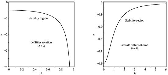
Figure 1.
We have defined and , respectively. The regions of stability are depicted in the graphs, below the curves for the de-Sitter and the anti-de Sitter solutions, respectively (plots adapted from Figure 3 of Ref. [18]).
3.3.2. Anti-de Sitter Spacetime
3.3.3. Schwarzschild Spacetime
This is the particular case of the Poisson–Visser analysis [17], with , which reduces to
The stability regions are shown in the left plot of Figure 2.
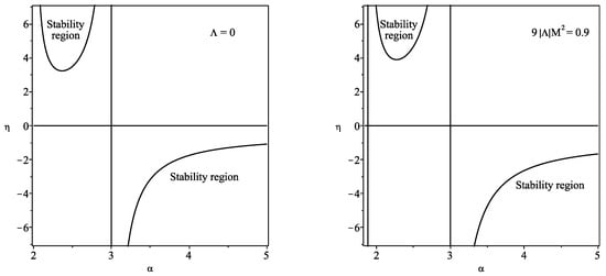
Figure 2.
We have defined . The regions of stability are depicted for the Schwarzschild and the Schwarzschild–anti-de Sitter solutions, respectively. Imposing the value in the Schwarzschild–anti-de Sitter case, we verify that the stability regions decrease relative to the Schwarzschild solution (plots adapted from Figure 4 of Ref. [18]).
3.3.4. Schwarzschild–Anti-de Sitter Spacetime
For the Schwarzschild–anti-de Sitter spacetime, with , we have
The regions of stability are depicted in the right plot of Figure 2, considering the value . In this case, the black hole event horizon is given by . We verify that the regions of stability decrease relative to the Schwarzschild case.
3.3.5. Schwarzschild–de Sitter Spacetime
For the Schwarzschild–de Sitter spacetime, with , we have
The regions of stability are depicted in Figure 3 for increasing values of . In particular, for , the black hole and cosmological horizons are given by and , respectively. Thus, only the interval is taken into account, as shown in the range of the respective plot. Analogously, for , we find and . Therefore, only the range within the interval corresponds to the stability regions, also shown in the respective plot.
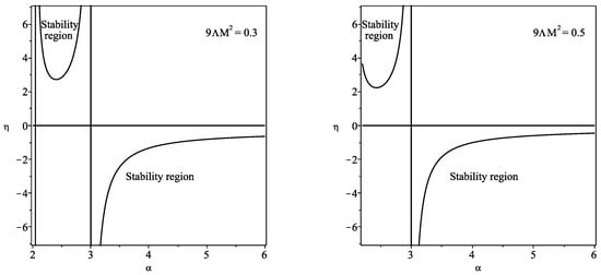
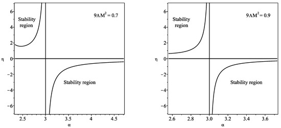
Figure 3.
We have defined . The regions of stability for the Schwarzschild–de Sitter solution, imposing , , and , respectively. The regions of stability are significantly increased, relative to the case, for increasing values of (plots adapted from Figure 5 of Ref. [18]).
We verify that for large values of , or large M, the regions of stability are significantly increased relative to the case.
4. A Thin Shell Around a Traversable Wormhole
As an alternative to the thin-shell wormhole, constructed using the cut-and-paste technique analyzed above, one may also consider that the exotic matter is distributed from the throat to a radius a, where the solution is matched to an exterior vacuum spacetime. Thus, the thin shell confines the exotic matter threading the wormhole to a finite region, with a delta function distribution of the stress–energy tensor on the junction surface.
We shall match the interior wormhole solution [1]
to the exterior vacuum solution
at a junction surface, . Note that the interior solution, given by Equation (46), should also be matched, at the throat , to two distinct ”upper” and “lower” spacetimes, where the metric functions could assume different values, namely, and . However, throughout this work we consider that the solutions are symmetric, so that and . See Figure 4 for specific details, where the plot demonstrates the symmetric matching at the throat , where both spacetimes are identified at the (ror asymmetric matchings, we refer the reader to Ref. [28]). Thus, the intrinsic metric to is given by
Note that the junction surface, , is situated outside the event horizon, i.e., , to avoid a black hole solution.
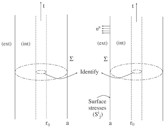
Figure 4.
Two copies of static timelike hypersurfaces, , embedded in asymptotic regions, separating an interior wormhole solution from an exterior vacuum spacetime. Both copies are identified at the wormhole throat, . The surface stresses reside on , and members of the normal vector field, , are shown (plot adapted from Figure 1 of Ref. [20]).
The Einstein equations, Equations (9) and (10), with the extrinsic curvatures, Equations (49)–(52), then provide us with the following expressions for the surface stresses:
where, for notational simplicity, we have defined the parameter by .
If the surface stress–energy terms are null, the junction is denoted as a boundary surface. If surface stress terms are present, the junction is called a thin shell, which is represented in Figure 4.
The surface mass of the thin shell is given by
One may interpret M as the total mass of the system, in this case, the total mass of the wormhole in one asymptotic region. Thus, solving Equation (55) for M, we finally have
In this section, we introduce several definitions to simplify the notation of the parameters used in the thin-shell formalism. For clarity, these dimensionless parameters are summarized in Table 1 to assist the reader during the analysis.

Table 1.
Definitions of the dimensionless parameters used throughout this section for the solutions under analysis.
4.1. Energy Conditions at the Junction Surface
The junction surface may serve to confine the interior wormhole exotic matter to a finite region, which in principle may be made arbitrarily small, and one may impose that the surface stress–energy tensor obeys the energy conditions at the junction, [2,61].
We shall only consider the weak energy condition (WEC) and the null energy condition (NEC). The WEC implies and and by continuity implies the null energy condition (NEC), .
From Equations (53) and (54), we deduce
We shall next find domains in which the NEC is satisfied by imposing that the surface energy density is non-negative, , i.e., .
4.1.1. Schwarzschild Solution
Consider the Schwarzschild solution, ; we impose that the surface energy density is non-negative, . For the particular case of , from Equation (57), we verify that is readily satisfied for .
For , the NEC is verified in the following region:
For convenience, by defining a new parameter , Equation (58) takes the form
For , the NEC is satisfied for , i.e., . For , we need to impose the NEC in the region of Equation (59), with for .
4.1.2. Schwarzschild–de Sitter Solution
For the Schwarzschild–de Sitter spacetime, , we shall once again impose a non-negative surface energy density, . Consider the definitions and .
For , the condition is readily met for , with given by
Choosing a particular example, for instance, , consider Figure 5. The region of interest is shown below the solid line, which is given by . The case of is depicted as a dashed curve, and the NEC is obeyed to the right of the latter.
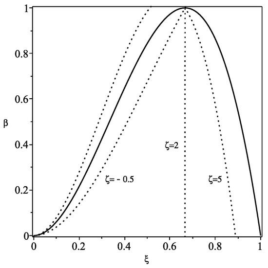
Figure 5.
Analysis of the null energy condition for the Schwarzschild–de Sitter spacetime. We have considered the definitions and . Only the region below the solid line is of interest. We have considered specific examples, and the NEC is obeyed to the right of each respective dashed curve, , and (plot adapted from Figure 4 of Ref. [20]). See text for details.
For , then, the NEC is verified for and , i.e., , with given by Equation (12). This analysis is depicted in Figure 5, to the right of the dashed curve, represented by .
For the case of , the condition needs to be imposed in the region ; and for . The specific case of is depicted as a dashed curve in Figure 5. The NEC needs to be imposed to the right of the respective curve.
4.1.3. Schwarzschild–anti-de Sitter Solution
Considering the Schwarzschild–anti-de Sitter spacetime, , once again, a non-negative surface energy density, , is imposed. Consider the definitions and .
For , the condition is readily met for and . For , the NEC is satisfied in the region , with given by
The particular case of is depicted in Figure 6. The region of interest is delimited by the -axis and the area to the left of the solid curve, which is given by . Thus, the NEC is obeyed above the dashed curve represented by the value .
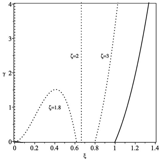
Figure 6.
Analysis of the null energy condition for the Schwarzschild–anti-de Sitter spacetime. We have considered the definitions and . The only area of interest is depicted to the left of the solid curve, given by . For the specific case of , the NEC is obeyed above the respective curve. For the cases of and , the NEC is verified to the right of the respective dashed curves, and to the left of the solid line (plot adapted from Figure 5 of Ref. [20]). See text for details.
For , then, is verified for and , i.e., , with given by Equation (14). Thus, the NEC is obeyed to the right of the dashed curve represented by , and to the left of the solid line, .
For the case of , the condition needs to be imposed in the region . The specific case of is depicted in Figure 6 as a dashed curve. Thus, the NEC needs to be imposed in the region to the right of the respective dashed curve and to the left of the solid line, .
4.2. Specific Cases
Taking into account Equations (53) and (54), one may express p as a function of by the following relationship
We shall analyze Equation (62), that is, find domains in which p assumes the nature of a tangential surface pressure, , or a tangential surface tension, , for the Schwarzschild case, , the Schwarzschild–de Sitter spacetime, , and for the Schwarzschild–anti-de Sitter solution, . In the analysis that follows, we shall consider that M is positive, .
4.2.1. Schwarzschild Spacetime
For the Schwarzschild spacetime, , Equation (62) reduces to
To find domains in which p is a tangential surface pressure, , or a tangential surface tension, , it is convenient to express Equation (63) in the compact form
with and . is defined as
One may now fix one or several of the parameters and analyze the sign of , and consequently the sign of p.
Fixed ζ, varying ξ and μ. For instance, consider a fixed value of , varying the parameters ; i.e., consider a fixed value of and vary the values of the junction radius, a, and of the surface energy density, . It is necessary to separate the cases of , and , respectively.
Firstly, for the case of , Equation (65) reduces to , which is always positive, as , implying a tangential surface pressure, .
Secondly, for , the qualitative behavior can be represented by the specific case of , corresponding to a constant redshift function and depicted in Figure 7. For non-positive values of and , a surface pressure, , is required to hold the thin shell structure against collapse. Close to the black hole event horizon, , i.e., , a surface pressure is also needed to hold the structure against collapse. For high values of and low values of , a surface tangential tension, , is needed to hold the structure against expansion. In particular, for the constant redshift function, , and a null surface energy density, , i.e., and , respectively, Equation (65) reduces to , from which we readily conclude that p is non-negative everywhere, tending to zero at infinity, i.e., . This is a particular case analyzed in [22]. Note that a surface boundary, with and , is given by , for .
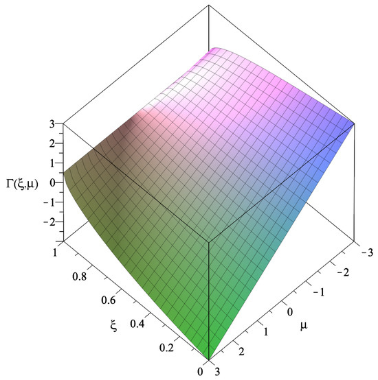
Figure 7.
The surface represents the sign of p for the Schwarzschild spacetime, , with a constant redshift function, , i.e., . For non-positive values of and , we have a surface tangential pressure, . For extremely high values of (close to the black hole event horizon) and , a surface pressure is also required to hold the structure against collapse. For high and low , we have a tangential surface tension, . See text for details.
Finally, for the case, the qualitative behavior can be represented by the specific case of , depicted in Figure 8. For non-negative values of and for , a surface pressure, , is required. For low negative values of and for low values of , a surface tension is needed, which is somewhat intuitive as a negative surface energy density is gravitationally repulsive, requiring a surface tension to hold the structure against expansion.
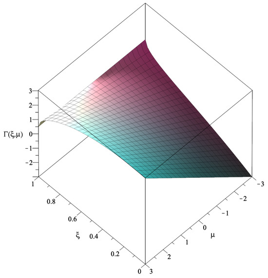
Figure 8.
The surface is given by Equation (65) for the Schwarzschild spacetime, , with . For non-negative values of and , we have a surface tangential pressure, . For negative values of and low , a tangential surface tension, , is required to hold the structure against expansion. See text for details.
4.2.2. Schwarzschild–de Sitter Spacetime
For the Schwarzschild–de Sitter spacetime with , to analyze the sign of p, it is convenient to express Equation (62) in the following compact form:
with , and . is defined as
One may now fix several of the parameters and analyze the sign of , and consequently the sign of p.
Null surface energy density. For instance, consider a null surface energy density, , i.e., . Thus, Equation (67) reduces to
To analyze the sign of p, we shall consider a null tangential surface pressure, i.e., , so that from Equation (68), we have the relationship
with , which is identical to Equation (60).
For the particular case of , from Equation (68), we have . A surface boundary, , is presented at ; i.e., . A surface pressure, , is given for , i.e., , and a surface tension, , for , i.e., .
For , from Equation (68), a surface pressure, , is met for , and a surface tension, , for . The specific case of a constant redshift function, i.e., , is analyzed in [22] (for this case, Equation (69) is reduced to , or ). For the qualitative behavior, the reader is referred to the particular case of provided in Figure 5. To the right of the curve a surface pressure, , is given, and to the left of the respective curve a surface tension, .
For , from Equation (68), a surface pressure, , is given for , and a surface tension, , for . Once again, the reader is referred to Figure 5 for a qualitative analysis of the behavior for the particular case of . A surface pressure is given to the right of the curve and a surface tension to the left.
Note that for the analysis considered in this section, namely, for a null surface energy density, the WEC and consequently the NEC are satisfied only if . The results obtained are consistent with those of the section regarding the energy conditions at the junction surface, for the Schwarzschild-de Sitter spacetime, considered above.
4.2.3. Schwarzschild–anti-de Sitter Spacetime
For the Schwarzschild–anti-de Sitter spacetime, , and to analyze the sign of p, Equation (62) is expressed as
with the parameters given , and , respectively. is defined as
As in the Schwarzschild–de Sitter solution, we shall analyze the case of a null surface energy density, , i.e., .
Null surface energy density. For a null surface energy density, , i.e., , Equation (71) reduces to
To analyze the sign of p, once again, we shall consider a null tangential surface pressure, i.e., , so that from Equation (72), we have
with , which is identical to Equation (61).
For the particular case of , from Equation (72), we have , which is null at , i.e., . A surface pressure, , is given for , i.e., , and a surface tension, , for , i.e., . The reader is referred to the particular case of , depicted in Figure 6. A surface pressure is given to the right of the respective dashed curve, and a surface tension to the left.
For , a surface pressure, , is given for and . For , a surface pressure, , is given for ; and a surface tension, , is provided for . The particular case of is depicted in Figure 6, in which a surface pressure is presented above the respective dashed curve, and a surface tension is presented in the region delimited by the curve and the -axis.
For , a surface pressure, , is met for , and a surface tension, , for . The specific case for is depicted in Figure 6. The surface pressure is presented to the right of the respective curve and the surface tension to the left.
Once again, the analysis considered in this section is consistent with the results obtained in the section regarding the energy conditions at the junction surface, for the Schwarzschild-anti de Sitter spacetime, considered above. This is due to the fact that for the specific case of a null surface energy density, the regions in which the WEC and NEC are satisfied coincide with the range of .
4.3. Pressure Balance Equation
One may obtain an equation governing the behavior of the radial pressure in terms of the surface stresses at the junction boundary from the following identity [2,62]: , where is the total stress–energy tensor, and the square brackets denotes the discontinuity across the thin shell, i.e., . Taking into account the values of the extrinsic curvatures, Equations (49)–(52), and noting that the tension acting on the shell is by definition the normal component of the stress–energy tensor, , we finally have the following pressure balance equation
where the ± superscripts correspond to the exterior and interior spacetimes, respectively. Equation (74) relates the difference in the radial tension across the shell in terms of a combination of the surface stresses, and p, given by Equations (53) and (54), respectively, and the geometrical quantities.
Note that for the exterior vacuum solution, we have . For the particular case of a null surface energy density, , and considering that the interior and exterior cosmological constants are equal, , Equation (74) reduces to
For a radial tension, , acting on the shell from the interior, a tangential surface pressure, , is needed to hold the collapsing thin shell form. For a radial interior pressure, , then, a tangential surface tension, , is needed to hold the structure form expansion.
4.4. Traversability Conditions
In this section, we shall consider the traversability conditions required for the traversal of a human being through the wormhole and consequently determine specific dimensions for the wormhole. Specific cases for the traversal time and velocity will also be estimated.
Consider the redshift function given by , with . Thus, from the definition of , the redshift function, in terms of , takes the form
with . With this choice of , may also be defined as . The case of corresponds to the constant redshift function so that . If , then is finite throughout spacetime and in the absence of an exterior solution, we have . As we are considering a matching of an interior solution with an exterior solution at a, then it is also possible to consider the case, imposing that is finite in the interval .
In the following analysis, we consider a thought experiment in which a traveler journeys radially through a wormhole. Thus, the analysis outlined below is valid for a radially moving observer. One of the traversability conditions was that the acceleration felt by the traveler should not exceed Earth’s gravity [1]. Consider an orthonormal basis of the traveler’s proper reference frame, , given in terms of the orthonormal basis of the static observers, by a Lorentz transformation. The traveler’s four-acceleration expressed in his proper reference frame, , yields the following restriction
where , and v is the velocity of the traveler [1]. The condition is immediately satisfied at the throat, . From Equation (77), one may also find an estimate for the junction surface, a. Considering that and , i.e., for low traversal velocities, and taking into account Equation (76), from Equation (77), one deduces . Considering the equality case, one has
Providing a value for , one may find an estimate for a. For instance, considering that , one finds that .
Another of the traversability conditions that was required was that the tidal accelerations felt by the traveler should not exceed the Earth’s gravitational acceleration. The tidal acceleration felt by the traveler is given by , where is the traveler’s four-velocity and is the separation between two arbitrary parts of his body. For simplicity, we shall assume that along any spatial direction in the traveler’s reference frame, and that . Consider the radial tidal constraint, , which can be regarded as constraining the metric field , i.e.,
At the throat, , and taking into account Equation (76), then Equation (79) reduces to or
considering the equality case.
Using Equations (78) and (80), one may find an estimate for the throat radius by providing a specific value for . Considering and equating Equations (78) and (80), one finds
Kuhfittig [63,64,65] proposed models restricting the exotic matter to an arbitrarily thin region under the condition that is close to unity near the throat. If , then the embedding diagram will flare out very slowly, so that, from Equation (81), may be made arbitrarily small. Nevertheless, using the form functions specified in [1], we will consider that . Using the above value of , then from Equation (81) we find .
To determine the traversal time of the total trip, suppose that the traveler accelerates at halfway to the throat, then decelerates at the same rate coming to rest at the throat [1,64]. For simplicity, we shall consider near the throat, so the wormhole will flare out very slowly. Therefore, from Equation (81), the throat will be relatively small, so we may assume that , as in [64]. Consider that a space station is situated just outside the junction surface at a, from which the intrepid traveler will start their journey. Thus, the total time of the trip will be approximately . The maximum velocity attained by the traveler will be approximately .
5. Conclusions
Traversable wormhole spacetimes typically require the presence of exotic matter, i.e., material that violates the NEC. However, by introducing a junction surface, it is possible to confine this exotic matter to a finite region, matching the interior wormhole geometry to an exterior, asymptotically well-behaved spacetime. As a result, the exotic matter can, in principle, be restricted to an arbitrarily small volume. The volume integral quantifier provides a means to evaluate the total amount of energy condition-violating matter present [19]. Using this formalism, explicit wormhole solutions have been constructed where appropriate choices of the interior metric and matching radius yield configurations supported by arbitrarily small quantities of matter that violate the averaged null energy condition (ANEC) [19].
Nevertheless, violations of the NEC, its averaged form (ANEC), and the WEC are inherent features of traversable wormholes. These arise directly from the flaring-out condition at the throat, which entails the violation of the NEC. To minimize the presence of exotic matter, as mentioned above, one can consider models where these violations are confined to a narrow region near the throat, , while the thin shell at the junction surface may, in principle, satisfy the standard energy conditions. In the limit , the exotic matter region becomes arbitrarily small. In this construction, the stress–energy tensor on the shell can be interpreted as describing quasi-normal matter, meaning that it obeys both the NEC and the WEC [2,19,61].
It is worth noting that in this context, analyzing the dominant energy condition (DEC) becomes largely redundant. The DEC, which imposes that energy flows along causal (timelike or null) worldlines and demands that the energy density dominate over the pressures, is a stricter constraint than both the WEC and NEC. Since the NEC is already violated in all traversable wormhole geometries, this automatically implies the breakdown of both the WEC and DEC as well. Therefore, the violation of the DEC is not an independent or surprising feature in wormhole physics, and it is sufficient to focus the analysis on the NEC and WEC violations that are inherently tied to the wormhole’s geometric structure.
In summary, in this work, we have explored the construction and physical viability of thin-shell wormholes influenced by a cosmological constant, employing the cut-and-paste technique. Our analysis revealed that the inclusion of a positive cosmological constant, as in the Schwarzschild–de Sitter geometry, notably enlarges the parameter space of stable configurations compared to the classic Schwarzschild case. Conversely, for a negative cosmological constant, corresponding to the Schwarzschild–anti-de Sitter background, the stability regions contract, indicating a more constrained and potentially less favorable environment for sustaining traversable wormholes.
To reduce the reliance on exotic matter, a generic feature in wormhole physics, we further constructed composite spacetimes by joining an interior wormhole geometry to an exterior vacuum solution at a finite junction surface. By examining the surface stresses, we identified domains where the weak and null energy conditions could be respected. A governing equation was derived for the radial pressure’s behavior across the junction, adding further insight into the mechanical equilibrium of the configuration.
Finally, in evaluating traversability, we considered realistic constraints such as the proper throat and junction radii, traversal time, and allowable velocities. These estimates ensure that the constructed wormholes are not only theoretically consistent but also potentially traversable. Altogether, our findings broaden the framework for building physically plausible and stable wormholes, and demonstrate the crucial role a cosmological constant may play in shaping their viability within general relativity.
In conclusion, the thin-shell construction remains a powerful and versatile method for modeling wormholes, particularly in scenarios where one aims to minimize exotic matter. Its ability to clearly examine the properties of the junction surface makes it useful for theoretical investigations into the interplay between gravitation, energy conditions, and topology change. Looking ahead, future work could extend these models by incorporating more general matter fields, analyzing dynamical stability under time-dependent perturbations, or embedding them in modified theories of gravity. Such directions not only deepen our understanding of fundamental physics but also pave the way for exploring whether traversable wormholes might one day be realized within a consistent and physically plausible framework.
Funding
FSNL acknowledges support from the Fundação para a Ciência e a Tecnologia (FCT) Scientific Employment Stimulus contract with reference CEECINST/00032/2018, and the research grants No. UID/FIS/04434/2020, No. PTDC/FIS-OUT/29048/2017 and No. CERN/FIS-PAR/0037/2019.
Conflicts of Interest
The authors declare no conflicts of interest.
References
- Morris, M.S.; Thorne, K.S. Wormholes in space-time and their use for interstellar travel: A tool for teaching general relativity. Am. J. Phys. 1988, 56, 395–412. [Google Scholar] [CrossRef]
- Visser, M. Lorentzian Wormholes: From Einstein to Hawking; American Institute of Physics: New York, NY, USA, 1995. [Google Scholar]
- Lobo, F.S.N. Wormholes, Warp Drives and Energy Conditions. Fundam. Theor. Phys. 2017, 189, 279. [Google Scholar]
- Barcelo, C.; Visser, M. Twilight for the energy conditions? Int. J. Mod. Phys. D 2002, 11, 1553–1560. [Google Scholar] [CrossRef]
- Morris, M.S.; Thorne, K.S.; Yurtsever, U. Wormholes, Time Machines, and the Weak Energy Condition. Phys. Rev. Lett. 1988, 61, 1446–1449. [Google Scholar] [CrossRef]
- Krasnikov, S. The Time travel paradox. Phys. Rev. D 2002, 65, 064013. [Google Scholar] [CrossRef]
- Alcubierre, M. The Warp drive: Hyperfast travel within general relativity. Class. Quant. Grav. 1994, 11, L73–L77. [Google Scholar] [CrossRef]
- Krasnikov, S.V. Hyperfast travel in general relativity. Phys. Rev. D 1998, 57, 4760–4766. [Google Scholar] [CrossRef]
- Olum, K.D. Superluminal travel requires negative energies. Phys. Rev. Lett. 1998, 81, 3567–3570. [Google Scholar] [CrossRef]
- Visser, M. Traversable wormholes: Some simple examples. Phys. Rev. D 1989, 39, 3182–3184. [Google Scholar] [CrossRef]
- Visser, M. Traversable wormholes from surgically modified Schwarzschild space-times. Nucl. Phys. B 1989, 328, 203–212. [Google Scholar] [CrossRef]
- Darmois, G. Mémorial des Sciences Mathématiques XXV. Fasticule XXV ch V; Gauthier-Villars: Paris, France, 1927. [Google Scholar]
- Israel, W. Singular hypersurfaces and thin shells in general relativity. Nuovo Cim. B 1966, 44, 1–14, Erratum in Nuovo Cim. B 1967, 48, 463. [Google Scholar] [CrossRef]
- Kim, S.W. Schwarzschild-de Sitter type wormhole. Phys. Lett. A 1992, 166, 13–16. [Google Scholar] [CrossRef]
- Visser, M. Quantum Mechanical Stabilization of Minkowski Signature Wormholes. Phys. Lett. B 1990, 242, 24–28. [Google Scholar] [CrossRef]
- Kim, S.W.; Lee, H.J.; Kim, S.K.; Yang, J.M. (2+1)-dimensional Schwarzschild-de Sitter wormhole. Phys. Lett. A 1993, 183, 359–362. [Google Scholar] [CrossRef]
- Poisson, E.; Visser, M. Thin shell wormholes: Linearization stability. Phys. Rev. D 1995, 52, 7318–7321. [Google Scholar] [CrossRef]
- Lobo, F.S.N.; Crawford, P. Linearized stability analysis of thin shell wormholes with a cosmological constant. Class. Quant. Grav. 2004, 21, 391–404. [Google Scholar] [CrossRef]
- Visser, M.; Kar, S.; Dadhich, N. Traversable wormholes with arbitrarily small energy condition violations. Phys. Rev. Lett. 2003, 90, 201102. [Google Scholar] [CrossRef]
- Lobo, F.S.N. Surface stresses on a thin shell surrounding a traversable wormhole. Class. Quant. Grav. 2004, 21, 4811–4832. [Google Scholar] [CrossRef]
- Lobo, F.S.N. Energy conditions, traversable wormholes and dust shells. Gen. Rel. Grav. 2005, 37, 2023–2038. [Google Scholar] [CrossRef]
- Lemos, J.P.S.; Lobo, F.S.N.; de Oliveira, S.Q. Morris-Thorne wormholes with a cosmological constant. Phys. Rev. D 2003, 68, 064004. [Google Scholar] [CrossRef]
- Lemos, J.P.S.; Lobo, F.S.N. Plane symmetric traversable wormholes in an Anti-de Sitter background. Phys. Rev. D 2004, 69, 104007. [Google Scholar] [CrossRef]
- Lemos, J.P.S.; Lobo, F.S.N. Plane symmetric thin-shell wormholes: Solutions and stability. Phys. Rev. D 2008, 78, 044030. [Google Scholar] [CrossRef]
- Lemos, J.P.S. Two-dimensional black holes and planar general relativity. Class. Quant. Grav. 1995, 12, 1081–1086. [Google Scholar] [CrossRef]
- Lemos, J.P.S.; Zanchin, V.T. Rotating charged black string and three-dimensional black holes. Phys. Rev. D 1996, 54, 3840–3853. [Google Scholar] [CrossRef] [PubMed]
- Lemos, J.P.S. Gravitational collapse to toroidal, cylindrical and planar black holes with gravitational and other forms of radiation. Phys. Rev. D 1998, 57, 4600–4605. [Google Scholar] [CrossRef]
- Garcia, N.M.; Lobo, F.S.N.; Visser, M. Generic spherically symmetric dynamic thin-shell traversable wormholes in standard general relativity. Phys. Rev. D 2012, 86, 044026. [Google Scholar] [CrossRef]
- Lobo, F.S.N.; Crawford, P. Stability analysis of dynamic thin shells. Class. Quant. Grav. 2005, 22, 4869–4886. [Google Scholar] [CrossRef]
- Eiroa, E.F. Stability of thin-shell wormholes with spherical symmetry. Phys. Rev. D 2008, 78, 024018. [Google Scholar] [CrossRef]
- Thibeault, M.; Simeone, C.; Eiroa, E.F. Thin-shell wormholes in Einstein-Maxwell theory with a Gauss-Bonnet term. Gen. Rel. Grav. 2006, 38, 1593–1608. [Google Scholar] [CrossRef]
- Dias, G.A.S.; Lemos, J.P.S. Thin-shell wormholes in d-dimensional general relativity: Solutions, properties, and stability. Phys. Rev. D 2010, 82, 084023. [Google Scholar] [CrossRef]
- Rahaman, F.; Kalam, M.; Chakraborty, S. Thin shell wormholes in higher dimensiaonal Einstein-Maxwell theory. Gen. Rel. Grav. 2006, 38, 1687–1695. [Google Scholar] [CrossRef]
- Eiroa, E.F.; Richarte, M.G.; Simeone, C. Thin-shell wormholes in Brans-Dicke gravity. Phys. Lett. A 2008, 373, 1–4, Erratum in Phys. Lett. 2009, 373, 2399–2400. [Google Scholar] [CrossRef]
- Yue, X.; Gao, S. Stability of Brans-Dicke thin shell wormholes. Phys. Lett. A 2011, 375, 2193–2200. [Google Scholar] [CrossRef][Green Version]
- Eiroa, E.F.; Aguirre, G.F. Thin-shell wormholes with charge in F(R) gravity. Eur. Phys. J. C 2016, 76, 132. [Google Scholar] [CrossRef]
- Eiroa, E.F.; Figueroa Aguirre, G. Thin-shell wormholes with a double layer in quadratic F(R) gravity. Phys. Rev. D 2016, 94, 044016. [Google Scholar] [CrossRef]
- Rosa, J.L.; André, R.; Lemos, J.P.S. Traversable wormholes with double layer thin shells in quadratic gravity. Gen. Rel. Grav. 2023, 55, 65. [Google Scholar] [CrossRef]
- Rosa, J.L.; Lemos, J.P.S.; Lobo, F.S.N. Wormholes in generalized hybrid metric-Palatini gravity obeying the matter null energy condition everywhere. Phys. Rev. D 2018, 98, 064054. [Google Scholar] [CrossRef]
- Rosa, J.L.; Lemos, J.P.S. Junction conditions for generalized hybrid metric-Palatini gravity with applications. Phys. Rev. D 2021, 104, 124076. [Google Scholar] [CrossRef]
- Rosa, J.L. Double gravitational layer traversable wormholes in hybrid metric-Palatini gravity. Phys. Rev. D 2021, 104, 064002. [Google Scholar] [CrossRef]
- Godani, N. Charged wormholes in Hybrid metric-Palatini gravity. Int. J. Geom. Methods Mod. Phys. 2023, 20, 2350193. [Google Scholar] [CrossRef]
- Rosa, J.L. Junction conditions and thin shells in perfect-fluid f (R, T) gravity. Phys. Rev. D 2021, 103, 104069. [Google Scholar] [CrossRef]
- Rosa, J.L.; Kull, P.M. Non-exotic traversable wormhole solutions in linear f (R, T) gravity. Eur. Phys. J. C 2022, 82, 1154. [Google Scholar] [CrossRef]
- Rosa, J.L.; Ganiyeva, N.; Lobo, F.S.N. Non-exotic traversable wormholes in f (R, TabTab) gravity. Eur. Phys. J. C 2023, 83, 1040. [Google Scholar] [CrossRef]
- Ganiyeva, N.; Rosa, J.L.; Lobo, F.S.N. Wormhole Geometries in f (R, T2) Gravity Satisfying the Energy Conditions. Contribution to the 17th Marcel Grossmann Meeting: On Recent Developments in Theoretical and Experimental General Relativity, Gravitation, and Relativistic Field Theories (MG17). arXiv 2023, arXiv:2502.19323. [Google Scholar]
- Eiroa, E.F.; Simeone, C. Stability of Chaplygin gas thin-shell wormholes. Phys. Rev. D 2007, 76, 024021. [Google Scholar] [CrossRef]
- Eiroa, E.F. Thin-shell wormholes with a generalized Chaplygin gas. Phys. Rev. D 2009, 80, 044033. [Google Scholar] [CrossRef]
- Bejarano, C.; Eiroa, E.F. Dilaton thin-shell wormholes supported by a generalized Chaplygin gas. Phys. Rev. D 2011, 84, 064043. [Google Scholar] [CrossRef]
- Halilsoy, M.; Ovgun, A.; Mazharimousavi, S.H. Thin-shell wormholes from the regular Hayward black hole. Eur. Phys. J. C 2014, 74, 2796. [Google Scholar] [CrossRef]
- Usmani, A.A.; Hasan, Z.; Rahaman, F.; Rakib, S.A.; Ray, S.; Kuhfittig, P.K.F. Thin-shell wormholes from charged black holes in generalized dilaton-axion gravity. Gen. Rel. Grav. 2010, 42, 2901–2912. [Google Scholar] [CrossRef]
- Bejarano, C.; Eiroa, E.F.; Simeone, C. Thin-shell wormholes associated with global cosmic strings. Phys. Rev. D 2007, 75, 027501. [Google Scholar] [CrossRef]
- Eiroa, E.F.; Simeone, C. Cylindrical thin shell wormholes. Phys. Rev. D 2004, 70, 044008. [Google Scholar] [CrossRef]
- Eiroa, E.F.; Simeone, C. Some general aspects of thin-shell wormholes with cylindrical symmetry. Phys. Rev. D 2010, 81, 084022, Erratum in Phys. Rev. D 2014, 90, 089906. [Google Scholar] [CrossRef]
- Mazharimousavi, S.H.; Halilsoy, M.; Amirabi, Z. Stability of generic cylindrical thin shell wormholes. Phys. Rev. D 2014, 89, 084003. [Google Scholar] [CrossRef]
- Forghani, S.D.; Mazharimousavi, S.H.; Halilsoy, M. Asymmetric Thin-Shell Wormholes. Eur. Phys. J. C 2018, 78, 469. [Google Scholar] [CrossRef]
- Lobo, F.S.N.; Simpson, A.; Visser, M. Dynamic thin-shell black-bounce traversable wormholes. Phys. Rev. D 2020, 101, 124035. [Google Scholar] [CrossRef]
- Mehdizadeh, M.R.; Zangeneh, M.K.; Lobo, F.S.N. Higher-dimensional thin-shell wormholes in third-order Lovelock gravity. Phys. Rev. D 2015, 92, 044022. [Google Scholar] [CrossRef]
- Mazharimousavi, S.H.; Halilsoy, M.; Amirabi, Z. Higher dimensional thin-shell wormholes in Einstein-Yang-Mills-Gauss-Bonnet gravity. Class. Quant. Grav. 2011, 28, 025004. [Google Scholar] [CrossRef]
- Mehdizadeh, M.R.; Ziaie, A.H. Charged Wormhole Solutions in Einstein-Cartan gravity. Phys. Rev. D 2019, 99, 064033. [Google Scholar] [CrossRef]
- Hawking, S.W.; Ellis, G.F.R. The Large Scale Structure of Space-Time; Cambridge University Press: Cambridge, UK, 2023. [Google Scholar]
- Musgrave, P.; Lake, K. Junctions and thin shells in general relativity using computer algebra. 1: The Darmois-Israel formalism. Class. Quant. Grav. 1996, 13, 1885–1900. [Google Scholar] [CrossRef]
- Kuhfittig, P.K.F. A wormhole with a special shape function. Am. J. Phys. 1999, 67, 125–126. [Google Scholar] [CrossRef]
- Kuhfittig, P.K.F. Static and dynamic traversable wormhole geometries satisfying the Ford-Roman constraints. Phys. Rev. D 2002, 66, 024015. [Google Scholar] [CrossRef]
- Kuhfittig, P.K.F. Can a wormhole supported by only small amounts of exotic matter really be traversable? Phys. Rev. D 2003, 68, 067502. [Google Scholar] [CrossRef]


Disclaimer/Publisher’s Note: The statements, opinions and data contained in all publications are solely those of the individual author(s) and contributor(s) and not of MDPI and/or the editor(s). MDPI and/or the editor(s) disclaim responsibility for any injury to people or property resulting from any ideas, methods, instructions or products referred to in the content. |
© 2025 by the author. Licensee MDPI, Basel, Switzerland. This article is an open access article distributed under the terms and conditions of the Creative Commons Attribution (CC BY) license (https://creativecommons.org/licenses/by/4.0/).