Abstract
This article presents a comprehensive and rigorous overview of spacetime singularities within the framework of classical General Relativity. Singularities are defined through the failure of geodesic completeness, reflecting the limits of predictability in spacetime evolution. This paper reviews the mathematical structures involved, including differentiability classes of the metric, and explores key constructions such as Geroch’s and Schmidt’s formulations of singular boundaries. A detailed classification of singularities—quasi-regular, non-scalar, and scalar—is proposed, based on the behavior of curvature tensors along incomplete curves. The limitations of previous approaches, including the cosmic censorship conjecture and extensions beyond General Relativity, are critically examined. This work also surveys the major singularity theorems of Penrose and Hawking, emphasizing their implications for gravitational collapse and cosmology. By focusing exclusively on the classical regime, this article lays a solid foundation for the systematic study of singular structures in relativistic spacetimes.
1. Definition of Singularities
1.1. Splendor and Misery of Singularities
The problem of singularities in four-dimensional spacetime is undoubtedly one of the most intriguing in General Relativity, especially due to the numerous “twists” in the last decades on the subject.
While the concept of singularities is well established in classical field theories (hydrodynamics, electrodynamics, etc.), the same cannot be said of General Relativity. The difference lies in the following fact: in all other field theories, spacetime is given once and for all as the framework for the theory, and a singularity in the field generally only indicates a limitation of the theory; for example, in electrodynamics, a solution of Maxwell’s equations is said to be singular if the field is infinite, and therefore indeterminate, at some point in Minkowski spacetime. By analogy, we would like to be able to say in General Relativity that spacetime is singular if the metric tensor is indeterminate at a point.
The trouble is that General Relativity is a theory in which the field interacts with the framework in which it is described: the field itself determines the geometric properties of spacetime.
In fact, there is always the possibility of escaping the problem, and many physicists do not believe that physics can collapse at singularities. Various more or less viable hypotheses have been put forward to this effect:
(1) General Relativity does not predict singularities.
This view was widely held in the 1960s [1]. However, the study of gravitational collapse and the publication by Penrose [2] and Hawking [3] of theorems demonstrating that in certain circumstances, a spacetime singularity necessarily occurs (if the theory of General Relativity is valid and if the momentum-energy tensor of matter satisfies a positivity condition), provided a striking counter-example to Lifshitz and Khalatnikov’s conjecture. The latter courageously admitted their error and became among the most fervent supporters of the existence of singularities in cosmology [4].
(2) General Relativity can also be modified to avoid singularities. The necessary modifications must include the possibility of repulsive gravity (since it is the attractive character of gravity that seems to be at the origin of the existence of singularities). In the theory put forth by Brans and Dicke [5], gravity remains attractive, and singularities are predicted [6]. The Einstein–Cartan theory (see for example [7]) contains a spin–spin interaction that can be repulsive; however, there are still situations—such as purely gravitational and electromagnetic fields—in which singularities occur. Most other theories of gravitation appear in some way to conflict with observations or involve assumptions that are physically unacceptable.
(3) The cosmic censorship hypothesis: after Blaise Pascal, who postulated that nature abhors vacuum, this conjecture puts forward the idea that nature abhors ‘naked’ singularities. In other words, if we start from an initially non-singular and asymptotically flat situation, all the singularities likely to develop later as a result of gravitational collapse would be hidden from the view of an observer placed at infinity behind a horizon [8]. Under these conditions, the singularities could rightly be ignored, since they would cause no detectable effect for observers careful enough not to fall into a black hole.
The cosmic censorship hypothesis has been beaten back on several fronts. Ethically speaking, it corresponds to a perfectly selfish attitude towards unlucky observers who might actually fall into a black hole. Physically, it does not solve the problem of the initial singularity of the universe (“big bang”), which is naked. Finally, Hawking’s discovery of the process of particle creation by a black hole casts serious doubt on the validity of this hypothesis. Studies on strong cosmic censorship examine whether singularities remain hidden or become observable. Works by Christodoulou [9,10], Dafermos [11], and others—for recent reviews, [12,13]—have revealed complex structures.
(4) General Relativity could eventually be quantified.
When this vast and difficult program was undertaken, some physicists hoped that strong quantum effects could eliminate singularities. Hawking [14] argued that spacetime singularities represent a fundamental limitation on our ability to predict the future—a limitation analogous to that imposed by the uncertainty principle in Quantum Mechanics. However considerable theoretical work has been dedicated to determining how quantum gravitational effects might modify the nature of singularities, or even eliminate them (for a recent review, see, e.g., [15]).
In the present work, we will not tackle the problem of the quantization of General Relativity. All of the results will be formulated in a classical (non-quantum) framework. In this simpler context, problems relating to the occurrence and description of singularities have been addressed for the last decades. But, while positive results were quickly found for their occurrence (Penrose and Hawking, already cited), the road to a good description of singularities was strewn with pitfalls: no sooner had a sketch of a description been formulated than counter-examples flourished in the field of publications.
Finally, after much trial and error, concepts were transformed into definitions, conjectures into theorems, arguments into proofs and hopes into results; in short, beliefs into knowledge.
In the following, we will attempt to untangle the skein, focusing only on the mathematical background without discussing the internal structure of singularities or the behavior of spacetime models near singularities, a subject we will cover in a second part of this review article. As most of the mathematical basis for dealing with classical spacetime singularities was provided in the 1970s, most of the references quoted in this paper date from this period. A general review of classical spacetime singularities without mathematical details but more recent references can be found, e.g., [16,17].
1.2. The Notion of Singularity
Before thinking about giving a good definition of what a singularity is in General Relativity, we need to have a notion of it.
A singularity can always be considered as the violation of a regularity condition of a basic structure of General Relativity. The structures in question can be the metric structure, the conformal structure, and the affine structure.
Given a model (M, g) and initial conditions on a compact spatial surface, we say that we obtain a singular development if (M, g) satisfies at least one of the following conditions:
- (i)
- (M, g) contains strong discontinuities (violation of the junction conditions)
- (ii)
- (M, g) is acausal (there are closed timelike lines)
- (iii)
- (M, g) is incomplete (the history of some particles cannot be described for all values of proper time).
For each of these structures, there is a complicated hierarchy of regularity conditions.
This notion of singularity is negative in the sense that it does not tell us what singular behavior actually is. This is precisely what we shall try to clarify through rigorous mathematics.
Note that case (i) is a purely local property, case (ii) is essentially global, and case (iii) is in principle global, but incompleteness can be “localized” by creating an extension of spacetime in which all incomplete curves have extremities and by attaching a singularity to an equivalence class of incomplete curves [18].
In commonly accepted definitions of singularities, case (ii) is omitted: for good reasons, the problem of causality is treated in a different context from that of singularities (see, for example, Section 6 of [19]), and we will not discuss it here. The emphasis will be placed on the incompleteness of spacetime.
This leaves the equivalence: a singularity is an incompleteness of spacetime whose metric satisfies certain regularity conditions.
Let us briefly explain what these conditions are.
1.3. Discontinuities in the Metric Structure
We may assume the manifold M of class C∞, since, according to Whitney’s embedding theorem, every atlas of class Ck (k ≥ 1) contains a sub-atlas of class C∞. But, the problem of choosing the C∞ structure is not so simple; although C∞ structure denotes a smooth atlas, a wrong choice of a particular coordinate chart can lead to factice “coordinate singularities”.
Concepts as diverse as geodesics, the Cauchy problem, or the continuity of the stress–energy tensor require, in order to be well defined, certain regularity conditions, which will be expressed by classes of differentiability of the metric g.
Recall that a function f defined on an open O of Rn is said to be locally Lipschitzian if, for any open U ⊂ O of compact closure, there exists a constant K such that ∀ p, q ⊂ U: |f(p) − f(q)| ≤ K |p − q|, where |p| denotes the Euclidean norm {∑(xi(p)2}1/2. A morphism ϕ is said to be locally Lipschitzian and denoted C1− if the coordinates of ϕ(p) are locally Lipschitzian functions of the coordinates of p. Similarly, we say that ϕ is Cr− if it is Cr−1 and if the derivatives of order r-1 of the coordinates of ϕ(p) are locally Lipschitzian functions of the coordinates of p.
C0 means continuous, C0− means locally bounded.
A spacetime (M, g) is said to be of class Ck (resp. Ck−), k ≥ 0, if the C∞-manifold M is Hausdorff and if:
(i) the components of the metric gab are continuous and admit locally bounded derivatives;
(ii) the components of the curvature tensor Rabcd are functions of class Ck (resp. Ck−).
To guarantee the existence and uniqueness of the geodesics, the following assumption is made:
gab is of strong curvature differentiability class sc-C2−, i.e., there exists an atlas C∞ of M such that the metric tensor is Lipschitzian (C1−) and the Riemann tensor Rabcd is locally bounded (C0−) [20].
In fact, a sc-C2− spacetime can be considered as the limit of a sequence of C2− spacetimes. Any result on geodesics that can be formulated in terms of the Riemann tensor alone will be valid on a sc-C2− spacetime as a limiting case of a sequence of geodesics.
To prove the existence and uniqueness of the solution of the Cauchy initial data problem, we use the following hypothesis:
There exists an atlas C∞ of M such that g and its derivatives up to order four exist in the sense of distributions and are locally square integrable; g is then said to be of Sobolev class W4 [21]; see also Section 7 of [19].
In order to obtain a dependence of class Ck in the initial data, these conditions must be strengthened in sc-C2+k− and W4+k.
In order to ensure the continuity of the normal components of the stress–energy tensor Tabf,a through the {f = const} surfaces, we must impose junction conditions: g is of class C1, C3 by pieces (see for example pp. 551–556 of [22]).
Finally, it should be noted that all these assumptions must be slightly weakened when describing certain phenomena such as shock waves [23].
In the following sections, it will always be assumed that the metric has the required differentiability class. In general, we will use C0-spacetimes (resp.C0−) when there are coordinates in which the gab are functions of class C2 (resp.C2−), corresponding to continuous (resp. locally bounded) Riemann tensors. The second case admits shock waves, the first does not.
The classification of singularities that we will describe later is designed to take account of both discontinuities in the metric and irregularities in the curvature tensor.
1.4. Spacetime Completeness
We have already seen that in General Relativity, the difficulty arises from the fact that we want to describe the singularities of a field which itself determines the geometric properties of spacetime.
The fact that components of the metric tensor become infinite at a point may simply be due to a poor choice of coordinate system. In any case, we can always amputate the manifold of a region in which the metric tensor is not defined and say that the remaining manifold represents the whole, non-singular spacetime. This shows that a definition of a singular spacetime cannot be based on the behavior of tensor field components and that singular points cannot be represented as belonging to the spacetime manifold itself. Since, on the other hand, we can always perform amputation surgery on spacetime, we would like to be sure that in such an operation, no non-singular part has been removed. Recognizing whether or not regions have been cut off from spacetime relates precisely to the problem of the completeness of spacetime.
1.5. Riemannian Manifolds
The case of a manifold M with a Riemannian metric g (positive definite) is very simple. A distance function d(p, q) can be defined as the lower bound of the lengths of the curves from p to q: d(p, q) = inf(∫pqds).
This function defines a metric in the topological sense, i.e., the balls B(p, r) = {q M|d(p, q) < r} form a basis of open sets for the topology of M.
A Cauchy sequence on M is an infinite sequence of points pn ∈ M such that ∀ε > 0, ∃ N|∀n, m > N, d(pn, pm) < ε.
We say that (M, g) is m-complete (m for “metric”) if every Cauchy sequence with respect to the distance function d converges to a point of M.
An equivalent formulation is as follows: (M, g) is m-complete if any curve γ: [a, b] → M of class C1 and finite length has an extremum, i.e., there exists a point p of γ such that for any neighborhood V of p, there exists t ∈ [a, b] such that ∀t1 ∈ [t, b], then y(t1) ∈ γ.
Singularities on a Riemannian manifold can therefore be described by the Cauchy completion, which exists and is unique.
We can also define a geodesic completeness (g-completeness) on a Riemannian manifold: (M, g) as g-complete if any geodesic of M can be extended to arbitrarily large values of its affine parameter.
Recall that a curve γ(t) is geodesic if γ is parallel to the tangent vector to the curve γ [D/∂t is the covariant derivative along γ(t)], and that the parameter t is said to be affine if .
An affine parameter on a geodesic curve is determined to within one additive constant and one multiplicative constant, i.e., within one affine transformation; in other words, if t is an affine parameter of γ, t′ = at + b is an affine parameter of γ, where a and b are arbitrary constants.
It can be shown [24] that for a positive definite metric, m-completeness and g-completeness are equivalent.
1.6. Pseudo-Riemannian Manifolds
The case of pseudo-Riemannian varieties is more complex.
A Lorentzian metric, for instance, does not define a metric in the topological sense, since there are inextensible curves of zero length (light rays). Even in the most regular case, the Minkowski spacetime, inextensible curves of finite length can be found: the curve x–t = (x + t)−2 from (x = 1, t = 0) to infinity has length √8.
Therefore, m-completeness cannot be defined for pseudo-Riemannian manifolds.
On the other hand, there are always geodesics, and we can obviously talk about g-completeness. However, there are three kinds of geodesics: timelike geodesics, null geodesics, and spacelike geodesics, so we are led to consider the three corresponding kinds of g-completeness:
- -
- t-g-completeness (completeness of timelike geodesics)
- -
- n-g-completeness (completeness of null geodesics)
- -
- s-g-completeness (completeness of spacelike geodesics)
One might expect a priori that a spacetime g-complete in one kind is g-complete in the other two kinds. Unfortunately, this is not the case [25,26]. Examples have been given of spacetimes that are:
- (1)
- t-g-complete but n,s-g-incomplete
- (2)
- s-g-complete but t,n-g-incomplete
- (3)
- n-g-complete but t,s-g-incomplete
- (4)
- t,n-g-complete but s-g-incomplete
- (5)
- s,n-g-complete but t-g-incomplete
To my knowledge, no example has yet been given of a t,s-g-complete but n-incomplete spacetime, and the non-existence of such a spacetime has not been demonstrated.
1.7. Physical Significance of Geodesic Incompleteness
The incompleteness of timelike geodesics has an immediate physical meaning: there are particles or free observers whose worldlines no longer exist after (or before) a finite interval of proper time. It seems appropriate to consider a spacetime containing such geodesics as singular.
Similarly, null geodesics are the trajectories of particles with zero rest mass. On the other hand, since the physical existence of free “tachyons” moving on spacelike geodesics has not been proven, the incompleteness of spacelike geodesics has no physical meaning for the moment.
It is therefore tempting to adopt the view that the completeness of timelike and null geodesics is the minimal condition for a spacetime to be non-singular.
Considering the incompleteness of timelike or null geodesics as indicating the presence of singularities has the advantage of leading to a number of fundamental theorems relating to the occurrence of this kind of singularity. These theorems, due to Penrose [2], Hawking [3,27], and Geroch [28], gave rise to a number of important works on the description of predicted singularities.
Hawking [3] and then Geroch [29] attempted to structure the set of singularities (i.e., relate it to the spacetime manifold, then provide it with a topology and possibly a metric) using the notion of geodesic incompleteness.
Note, however, that the problem of attaching a boundary to the spacetime (M, g) so as to describe singularities only concerns boundary points located at a finite distance from points of M. This boundary will not therefore represent points “at infinity” such as those of the conformal boundary studied in [30].
1.8. Geroch’s Construction
This consists in giving a structure to the set of incomplete geodesics. Roughly speaking, these incomplete geodesics are arranged in equivalence classes, each class defining a point in an abstract space ∂. The basic idea is that an incomplete geodesic γ can be defined by its initial conditions: any point on γ and the tangent vector to γ at that point. Let us consider the set of geodesics resulting from small variations in these initial conditions. This bundle is called the thickening of γ (Figure 1).
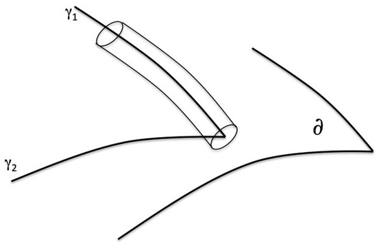
Figure 1.
Thickening of incomplete geodesic γ.
The two incomplete geodesics γ1 and γ2 are said to belong to the same equivalence class (and thus define the same singular point of ∂δ) if any thickening of one intersects any thickening of the other.
Let us now explain Geroch’s method more precisely. Let M be a spacetime. A geodesic in M is determined in a unique way by giving a point p of M and a non-zero vector Xp ∈ Tp(M): the geodesic starts from p with an initial direction Xp and an affine parameter λ determined by the following equation:
dxi/dλ/p = Xpi (I = 0, 1, 2, 3)
We denote G as the set of pairs (p, Xp); G is the part of the tangent fiber bundle of M comprising only the non-zero vectors; we therefore call it the reduced tangent fiber bundle of M. There is thus a one-to-one correspondence between the elements of G and the geodesics of M. These geodesics have an extremum, they are parametrized by an affine parameter, the latter cancelling at the extremum and being positive elsewhere along the curve.
We now want to characterize the subset GI of G corresponding to the incomplete geodesics of M.
To do this, we define the scalar field Φ on the manifold G to be the total affine length of the corresponding geodesic in M. GI is therefore the subset of G for which Φ is finite.
With a view to constructing a topology on GI, we introduce the manifold H = G × [0, ∞] and the following two subsets of H:
H+ = {(p, Xp, a) ∈ H|Φ(p, Xp) > a}
H0 = {(p, Xp, a) ∈ H|Φ(p, Xp) = a}
Note that in particular, the points (p, Χp, Φ(p,Xp)) are in H0.
There is a natural morphism Ψ: H+ → M, which maps to a point (p, Xp, a) in H+, the point in M constructed from p by measuring the affine length a along the geodesic (p, Xp).
This application will allow us to define the openings of a topology on GI. Let O be an open of M. Consider the subset S(O) of GI defined as follows:
S(O) = {(p, Xp) ∈ GI| there exists an open U in H containing the point (p, Xp, Φ(p, Xp)) of H0 such that Ψ(U H+) ⊂ O}
We can check that given two open sets O1 and O2 of M, we have S(O1) ⋂ S(O2) = S(O1 ⋂ O2). Therefore, when O crosses the set of open sets of H, S(O) is a basis of open sets of a GI topology.
This topology is used to form equivalence classes between elements of GI: if α and β are two elements of GI, α~β if any open set of GI containing α contains β, and vice versa. This is an equivalence relation. The set of equivalence classes is denoted ∂ and is called g-boundary (g for “geodesic” or for “Geroch”, take your pick!).
For example, the elements (p, Xp) and (p, λΧp) of GI, where λ is a non-zero constant, belong to the same equivalence class.
The topology defined on GI induces a topology on ∂ (the quotient-topology). Note, however, that there are various ways of forming equivalence classes to form a g-boundary. The identification described above is the “weakest”, in the sense that the points of GI are identified only if they are topologically indistinguishable, i.e., if they always appear in the same openings; the resulting g-boundary satisfies the separation axiom T0 (given any two distinct points x and y of ∂, there exists either a neighborhood of x that does not contain y or a neighborhood of y that does not contain x). Stronger identifications could define g-boundaries satisfying the separation axioms T1 (given any two distinct points x and y of ∂, there exists a neighborhood of x that does not contain y and a neighborhood of y that does not contain x), T2 or Hausdorff (there exists a neighborhood of x and a neighborhood of y that are disjoint), or T3 (∂ satisfies axiom T1 and is regular, i.e., for any point x of ∂, the closed neighborhoods of x form a basis of neighborhoods of x).
We now attach ∂ to the spacetime M by defining the disjoint union = M ⋃ ∂. The opens of are the subsets (O, U), where O is an open of M and U is an open of ∂ such that U ⊂ S(O).
We check that the intersection of two openings of is an open set of ; we therefore have a basis of open sets for a topology on . Spacetime with its g-boundary is a manifold with an edge.
According to Geroch, the g-boundary consists of the “singular” points of spacetime M. A proposition such as “the mass density becomes infinite at the singularity” translates mathematically as “the point x of the g-boundary has the property that whatever the number ρ0, there exists an open neighborhood (O,U) of x in such that ρ > ρ0 in O”.
Geroch then defines new structures on the g-boundary. Indeed, the topological properties of ∂ are not sufficient to classify singularities. Geroch therefore begins by giving ∂ a causal structure, i.e., determining on the one hand the “past” and “future” of each point of ∂, and defining on the other hand the “spatial” g-boundaries and the “temporal” g-boundaries.
Finally, Geroch provides ∂ with a differentiable structure and a metric, subject to certain conditions on spacetime.
1.9. The Sad Story of a Rocket
We will not go into the details of these constructions here. Indeed, Geroch’s attempt, interesting as it is, has certain limitations that the author himself acknowledges at the end of his article. We have already mentioned that there are several ways of defining equivalence classes on G1, hence a certain ambiguity in the local description of singular points. But the major obstacle is that the class of geodesically incomplete spacetimes does not cover all the kinds of singularities we would like to see.
Let us imagine an inextensible non-geodesic time curve with bounded acceleration and finite proper length. Could we not describe as singular the situation of the passenger in a rocket who, having travelled the entire length of the curve in a finite proper time, would no longer be represented by a point in the spacetime manifold? Geroch himself constructed a geodesically complete spacetime containing such a curve [26].
We would like to be able to say that this spacetime is singular. Therefore, a definition of the concept of singularity must include all incomplete curves, geodesic or not.
The most natural idea is to consider a notion of completeness according to which all curves of class C1, of finite length measured by an appropriate parameter, have an end.
1.10. Generalized Affine Parameter
The parameter in question used to measure the length of curves must be a generalization of the concept of the affine parameter, which until now has only been defined for geodesics. The concept of a generalized affine parameter is therefore introduced as follows:
Let γ(t): [a,b] → M be a curve of class C1 passing through a point p of M, and let {Ei}i=0,1,2,3 be a basis of the tangent space at p, Tp(M).
The basis {Ei} can be shifted parallel to itself along γ(t) to obtain a basis of Tγ(t) for all t in [a, b].
The tangent vector to the curve, V = (∂/∂t)γ(t) can therefore be expressed in terms of this basis as V = Vi(t)Ei.
We then define on γ(t) a generalized affine parameter v as follows:
where ||V(t)|| denotes the Euclidean norm of the tangent vector V:
v = ∫p||V(t)||dt,
||V(t)|| = {∑i(Vi(t)2}1/2.
If γ is a geodesic, v reduces to an affine parameter.
We can see that v depends on the point p and the basis {Ei}. However, it is easy to see that if v′ is another generalized affine parameter defined from a basis {Ei′} in p, the length of the curve g is finite in the parameter v′ if and only if it is finite in the parameter v. We therefore do not restrict the problem by considering only orthonormal bases {Ei}.
1.11. b-Completeness
We can now define b-completeness (b for “bundle”; see Section 1.12):
(M, g) is b-complete if any curve of class C1 of finite length measured by a generalized affine parameter has an extremum.
Note that if g is positive definite, the generalized affine parameter reduces to the curvilinear arc length so that b-completeness, g-completeness, and m-completeness are all equivalent.
For a Lorentzian metric, b-completeness obviously entails g-completeness, the opposite being false.
The completeness of spatial curves (s-completeness) leads to the completeness of null curves (n-cοmpleteness) and time curves (t-completeness). Thus, the affine completeness of all curves is equivalent to the completeness of spatial curves alone.
On the other hand, s-g-completeness does not imply t-g- or n-g-completeness.
The completeness of time curves leads to the completeness of curves with bounded acceleration (b.a-completeness), which in turn leads to the completeness of time geodesics. Note also that it is logical to call the completeness of null and timelike geodesics (t,n-g-completeness) “the completeness of causal geodesics” (c-g-completeness), for obvious physical reasons. The Hawking and Penrose singularity theorems involve incomplete causal geodesics.
Finally, it can be shown that the causal completeness of all curves is in fact equivalent to the completeness of null curves (see, for example, [31]).
We can thus schematize the hierarchy between the various types of completeness as follows (the ~ sign stands for “completeness”; arrows deduced by transitivity are not indicated); see Figure 2.
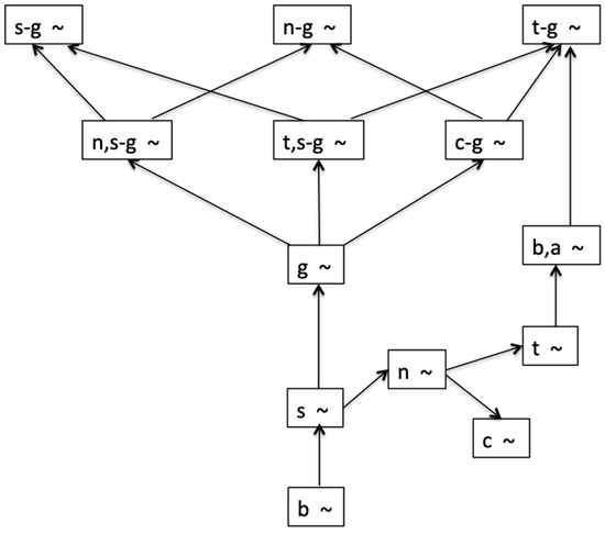
Figure 2.
Hierarchy between the various types of geodesic completeness.
1.12. Schmidt’s Construction
The rigorous construction of a b-boundary of spacetime representing the set of extremities of all incomplete curves of M was carried out by Schmidt [18,32]. His very elegant and sophisticated method is based on the fibred structure of linear reference frames L(M).
Recall that a fibred structure (see, for example, [33] on a topological space E (total space or fibred) is given by:
(a) a topological space B called base and a topological space F called fiber bundle-type;
(b) a continuous surjective application p: π: E → B called projection. For p ∈ B, π−1 (p) is called fiber of p;
(c) a covering of the basis B by a family of open U such that π−1(U) is homeomorphic to U × F, i.e., for any point p in U, there exists a homeomorphism Φp: π−1(p) → V such that the application ψ: π−1(U) → U × S is defined by ψ(x) = (π(x), Φπ(x)).
Thus, the fibered structure generalizes the notion of topological product. Indeed, the topological product E = X × Y is a fibred bundle with basis X, type-fiber Y, projection π(x,y) = x; the covering reduces to the single open U = X, the homeomorphism ψ is the identity, the structural group G reduces to the identity.
An application f: B → E such that π°f is the identity function on B is called a section of the fibered E. A fibered space where G = F is called a principal fibered bundle.
Consider a differentiable manifold Vn. A linear reference frame Rp at a point p of Vn is an ordered basis E1, …, En of the tangent space Tp(Vn). The set L(Vn) of all linear reference points at all points of Vn can be given a differentiable fibered structure: the basis is Vn, the type-fiber is the linear group of order n GL(n, R) (isomorphic to the group of regular n × n matrices with real coefficients), the projection is defined by π (p, Rp) = p, and the structural group is GL(n, R).
L(Vn) is therefore a differentiable main fibred bundle called fibered bundle of linear reference frames on manifold Vn. The structural group GL(n, R) acts on the right-hand side as follows:
A = {(aij)} ∈ GL(n, R) transforms (p,Ri) into (p, AijEj).
We can define a subbundle of L(Vn), the fiber of orthonormal reference frames O(Vn). In the case of a Lorentzian metric, the structural group is then the Lorentz group of dimension n: O(n − 1, 1).
If L(Vn) admits a section, Vn is said to be parallelizable. It can be shown that the existence of a connection on Vn implies that the manifold Vn is parallelizable.
Let us now go through the various stages of Schmidt’s construction, without however dwelling too much on the very technical aspects which have been amply described in the literature (chapter 8 of [19]).
Consider a spacetime manifold M and its orthonormal reference frame O(M). Since M has a connection, we can define so-called horizontal curves in O(M), obtained by transporting an orthonormal frame of reference in parallel along the curves of M.
Let Tu(O(M)) then be the tangent space at the point u of O(M), of dimension 10. The vectors tangent at u to the horizontal curves of O(M) passing through u give rise to a vector subspace of Tu(O(M)), of dimension 4, called the horizontal subspace Hu(O(M)).
Tu(O(M)) then decomposes into the direct sum of the horizontal subspace Hu(O(M)) and the vertical subspace Vu(O(M)) consisting of the vectors of Tu that are tangent to the fiber π−1 (π (u)).
This makes it possible to define a canonical set of linearly independent vectors constituting a basis of Tu(O(M)); such a basis {GA}A=1,2,…,10 can be written {GA} = {EA, i} where {Ea}a=1,…,4 is a basis of Hu and {i}i=1,…,6 is a basis of Vu.
With this basis, we can define a positive definite metric e on O(M) as follows:
e(X,Y) = ∑A XAYA, where X,Y ∈ Tu(O(M)} and XA, YA are the components of X,Y in the basis {GA}.
This metric makes it possible to introduce a distance function d on O(M): u and v being two points of O(M), d(u,v) is the lower bound of the lengths (measured by e) of the curves joining u and v.
O(M) thus becomes a metric space.
As we saw in Section 1.5, we can then complete O(H) by means of Cauchy sequences, defining the Cauchy completion as the set of equivalence classes of Cauchy sequences in O(M). is unique to within one isomorphism. We can write = O(M) ⋃ ∂O(M), where ∂O(M) = {u ∈ |u ∉ O(M)}.
The action of the Lorentz structural group O(3,1) can be extended to . We call the set of orbit under the action of O(3,1), and ∂M the set of orbits of ∂O(M). The projection p π: O(M) → M can be extended to → by defining (u) as the orbit passing by u ∈ .
being provided with a topology induced by the metric e, can also be provided with a topology by defining an open U of such that π−1(u) is an open set of . This is the weakest topology for which p is continuous.
We thus have a method for attaching a boundary ∂M to the spacetime M.
However, it would be premature to call all the points of ∂M “singular points”. Indeed, M could, for example, be extensible, so that singular points of ∂M could be perfectly regular in an extension of M.
Therefore, Schmidt was led to define a singularity as a point of ∂M that is contained in the boundary ∂ of any extension of M.
The fundamental question is to prove that ∂M coincides with the b-boundary consisting of the extremities of all incomplete curves of M. We have the theorem (Schmidt, 1971):
(O(M), e) is incomplete if and only if (M, g) is b-complete.
The proof of this theorem depends on the fact that every spacetime M is locally b-complete, i.e., every point of M has a neighborhood U of compact closure , such that the b-boundary ∂U of U coincides with the boundary /U of U in M [32].
We will not go into the details of the proofs here, as these can be found in the classical literature already mentioned.
Thus, any equivalence class of b-incomplete curves in M defines a point of ∂M.
Note that the topology of is not necessarily Hausdorff, i.e., there may exist a point p ∈ M and a point q ∈ ∂M such that any neighborhood of p in M intersects any neighborhood of q. This situation occurs when point q corresponds to an incomplete curve which is totally or partially trapped in M, as happens, for example, for the Taub–NUT space (for more details, see Sections 2.4 and 8.5 of [19]).
Other properties of the b-boundary have been discussed [34].
2. Classification of Singularities
2.1. Introduction
There is a feeling that the somewhat abstract definition of singularities in Schmidt’s sense must now be related to the intuitive physical conception one may have of a singularity, namely a point where the gravitational forces due to curvature become infinite.
We must therefore distinguish, among the points of the b-boundary, those where the Riemann tensor is irregular and thus establish a classification of singularities [35,36,37].
The idea is to base the classification on the behavior of the components of the Riemann tensor in a tetrad transported along an incomplete curve defining the singularity.
2.2. Extensible Manifolds
Before undertaking a classification of the points of the b-boundary, we must ensure that the spacetime manifold (M, g) is indeed inextensible (or maximal).
As already mentioned in Section 1.12, a point p on the b-boundary ∂M of an extensible spacetime M may be such that there exists an isometry ψ of (M, g) in a larger spacetime (M′, g′) which sends p onto an interior point of Μ′: (p) ∈ Μ′ (where is the extension of ψ on ∂M). Clearly, there is nothing “singular” about such a point in the physical sense. Clarke [20] named such points “locally inextensible inessential singularities”, but it is clear that the term “singularity” is superfluous. We will simply call such a point a regular boundary point.
Let us give two typical examples of such pathologies:
(a)—The Minkowski half-spacetime
The metric is: ds2 = −dt2 + dx2 + dy2 + dz2, defined for −∞ < x,y,z < +∞ and 0 < t < +∞.
The b-boundary consists of the plane {t = 0}, but it is clear that any boundary point is regular since it is contained in the extension of the half-spacetime into the full Minkowski spacetime.
(b)—The Schwarzschild exterior solution
This is the solution of the Einstein field equations for spherically symmetric empty space. In the static region, the metric is written as follows:
where −∞ < t < +∞, 0 < r < ∞, 0 ≤ θ ≤ π, 0 ≤ ϕ ≤ 2π.
ds2 = −(1 − 2m/r)dt2 + (1 − 2m/r) −1dr2 + r2(dθ2 + sin 2θdϕ2)
The b-boundary is the surface r = 2m, the well-known Schwarzschild horizon. But, we know that Schwarzschild spacetime is extensible (see, for example, [22]). Therefore, to avoid these pathologies, it is sufficient to construct the b-boundary only if the spacetime is maximal, in which case there will by definition no longer be any regular boundary point.
However, the problem is not easy: the choice of extension is not trivial, and the maximal analytic solution can be very complicated.
For example, Schwarzschild’s outer solution can be extended analytically into Kruskal’s maximal analytic solution [38], but an extension can also be made to obtain an ‘inner’ solution representing a static spherical star, or a spacetime containing a star evolving towards a black hole by the process of gravitational collapse.
The choice of extension therefore contains essential physical information.
Despite its interest, this problem will not be discussed further in the remainder of this paper.
2.3. The Three Classes of Singularities
After several attempts [20,36,39], the following terminology have been adopted [37].
Given a point p belonging to the b-boundary ∂M of an inextensible singular spacetime M, consider the components of the curvature tensor Rabcd(v) measured in a basis {Ea(v)} along a curve γ(v) ending at p, together with the components of the covariant derivatives of Rabcd to order k: Rabcd;e1…ek(v), and finally the Ck-curvature scalar fields, which are polynomial scalar fields constructed from the metric tensor gab, the completely antisymmetric tensor ηabcd, the Riemann tensor, and its covariant derivatives up to order k.
The point p of ∂M is said to be:
(a) Ck-quasi-regular singularity (resp, Ck−), k ≥ 0, if the Rabcd;e1…ek(v) components measured in a parallely transported basis along any curve ending at p are functions of class C0 (resp. C0−, i.e., locally bounded), but there is no Ck-extension (resp. Ck−-extension) of (M, g) in p.
(b) Ck-non-scalar singularity if there exists a curve γ(v) such that the Rabcd;e1…ek(v) components measured in a parallel transported basis along γ(v) are not all functions of class C0, but there exists no Ck-irregular curvature scalar field along all curves ending in p.
(c) Ck-scalar singularity if there is a curve γ(v) ending in p and a Ck-scalar field of curvature that is not of class C0 along γ(v).
This classification has the advantage of grouping together the various cases where the “singularity” of p refers to the behavior of the Riemann tensor and those where it refers to the differentiability of the metric at p (cf. Section 1.3).
Scalar and non-scalar singularities specifically involve an irregularity of curvature in the sense that observers moving towards the singularity along certain curves can measure components of the Riemann tensor that do not have a finite limit in parallel transported reference frames. In other words, it is the curvature of spacetime that prevents any extension to the point p (whereas in the case of quasi-regular singularities the obstacle is topological). These two classes can therefore be grouped together under the same heading of curvature singularities, also called p.p.curvature singularities (“parallelly propagated”) in the notation of Hawking and Ellis [19].
By considering which part of the Riemann tensor is irregular, we can refine the classification by defining Ricci (or matter) singularities if it is the components of the Ricci tensor that are irregular, and Weyl (or conformal) singularities if the irregularity only affects the Weyl tensor. Finally, we can distinguish cases where the non-convergence of the curvature tensor occurs because the irregular components are unbounded (divergent curvature singularities) or because they remain bounded but oscillate indefinitely without having a limit (oscillatory curvature singularities).
2.4. Quasi-Regular Singularities
A Ck-quasi-regular singularity is also said to be Ck-locally extensible, in the sense that any curve γ(v) ending at p and satisfying certain regularity conditions (causal curve) is contained in an open U of M such that γ can be extended beyond p in a Ck-local extension of (U, g) [35].
Here, “Ck-local extension” means local extension of differentiability class k, where k is the differentiability of the metric on M.
In other words, γ is contained in a neighborhood isometric to an open of a non-singular spacetime. Physically, an observer moving along γ towards p experiences no infinite gravitational force, because the components of the Riemann tensor measured in a tetrad transported parallel along γ are convergent. However, there is no global extension of (M, g) into (M′, g′) that would send p onto an interior point of M′: p is indeed an essential singularity attached to spacetime, but it does not lead to singular physical effects.
The simplest example of a quasi-regular singularity is the vertex of a cone. The most famous illustration is provided by the Taub–NUT–Misner spacetime (see for example Section 5.8 of [19] and Section 8 of [40]), about which we will say a few words.
In 1951, Taub discovered a solution to Einstein’s equations for empty space with the property of spatial homogeneity, i.e., at each point, there is a spatial hypersurface on which the metric is independent of position.
The metric of Taub space is written as follows:
where U(t) = −1 + 2(m + l2)(t2 + l2)−1, m and l are positive constants, 0 ≤ ψ ≤ 4π, 0 ≤ θ ≤ π, 0 ≤ ϕ ≤ 2π (the solution has the topology R × S3, so that ψ, θ a, d ϕ are Euler coordinates on S3).
ds2 = −U − 1dt2 + (2l)2U(dψ + cos θdϕ)2 + (t2 + l2)(dθ2 + sin 2θdϕ2)
This metric is singular in t = t± = m ± (m2 +l2)1/2, where U = 0.
Just as the Schwarzschild solution admits an extension through the horizon r = 2m, the Taub solution admits an extension beyond the surfaces t = t±. The resulting space was described independently by Newman, Unti, and Tamburino [41], and it was Misner and Taub [42] who highlighted the link between the two solutions: the Taub solution and the NUT solution can be “assembled” into a single manifold, the Taub–NUT–Misner space, in which there are two regions, one with the Taub metric, the other with the NUT metric, separated by a thousand hypersurfaces of topology S3 called Misner bridges.
The Taub–NUT–Misner space has incomplete geodesics ending in quasi-regular singularities.
A two-dimensional example given by Misner [43] has similar properties, so it is sufficient to describe this simpler case to get an idea of the situation in Taub–NUT–Misner spacetime.
Consider the two-dimensional Minkowski space (Figure 3).
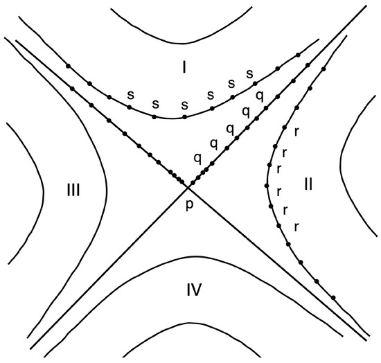
Figure 3.
Equivalence of points in 2D Minkowski space.
Under the action of the discrete subgroup G of the Lorentz group, the s points are equivalent, as are the q or r points.
By identifying the equivalent points in regions I and II, we obtain the cylinder: ds2 = −t−1dt2 + tdψ2, which has a closed null geodesic (t = 0) defining a locally extensible singularity (see Figure 4).
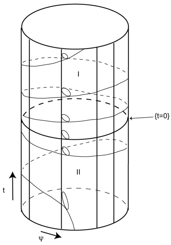
Figure 4.
Minkowski cylinder obtained via identification of points.
The vertical null geodesics are complete, but the null geodesics that spiral around the cylinder are incomplete. These geodesics can be extended locally by ‘unscrewing’ them, but this extension simply winds up the previously complete vertical null geodesics, rendering them incomplete.
Therefore, there is no global extension that would allow all the geodesics to be extended simultaneously beyond t = 0, but only a local extension that would allow one or another of the two families of null geodesics to be extended: t = 0 is indeed a locally extendable singularity.
In fact, it is possible to construct spacetimes with quasi-regular singularities by “cutting up” and “putting back together” pieces of regular spacetime (see, for example, [37]).
2.5. Existence of Quasi-Regular Singularities
The question arises as to whether these ‘unnatural’ singularities can develop from regular initial data.
In raising this question, we have in mind the problem of the nature of singularities in a cosmological model (i.e., a physically reasonable model capable of representing the whole of our universe during a given phase, and not just part of it). If quasi-regular singularities only occur in somewhat pathological spacetimes, they will be excluded from cosmological models.
Clarke [20] actually showed that, in general, any point p belonging to the boundary ∂V of a globally hyperbolic manifold V and accessible by a time curve of V cannot be a quasi-regular singular point.
Recall that a manifold V is said to be globally hyperbolic if it is causal and if the causal interval between any two points of V is compact; an equivalent formulation is that there exists a surface S in V called a partial Cauchy surface such that any causal curve intersects it once and only once.
The theorem is valid in general, i.e., quasi-regular singularities are only accessible by time curves if the Ricci and Weyl tensors have very particular forms (the spacetime is then said to be D-specialized, which is physically equivalent to an empty Petrov D-type spacetime).
Clarke [44] improved his theorem by including null curves: a maximal globally hyperbolic spacetime (with the required differentiability class) that is not D-specialized at any point has no quasi-regular singularity accessible by a causal curve.
Thus, the Cauchy expansion of regular initial data does not in general lead to a quasi-regular singularity.
We can interpret this result by saying that the existence of a quasi-regular singularity accessible by a causal curve of a globally hyperbolic spacetime must be unstable, since a small perturbation of the initial data may be enough to destroy the very special conditions that the curvature tensor must assume.
Another case where a quasi-regular singularity is accessible by causal curves occurs when incomplete causal curves are ‘trapped’ in a compact region of spacetime. A result of Hawking and Ellis (proposition 8.5.2 of [19]) shows that here again, the existence of the quasi-regular singularity must be unstable.
Finally, these examples suggest that quasi-regular singularities are either primordial, i.e., have existed since time immemorial (for a precise definition, see [44] or are unpredictable holes developing without apparently reasonable cause from regular Cauchy data. A theorem of Clarke, Th.4 of [44]) seems to confirm this hypothesis.
We shall see in the next section that the general theorems on singularities of Hawking and Penrose involve causal curves. The class of quasi-regular singularities is therefore ruled out in the context of these theorems. For this reason, we will not dwell further on this class, even though numerous examples of spacetime pathologies rivalling in perversity have been given to illustrate these quasi-regular rather singular singularities.
Finally, however, let us add that, since we can construct many relatively simple spacetimes admitting a quasi-regular singularity by cutting out particular regions of regular spacetimes and making certain identifications, we might hope to find a sub-classification of this type of singularity. In fact, it seems that this is not possible, see Appendices A and B of [37]).
2.6. Non-Scalar Singularities
The definition of non-scalar singularities suffices to show that the curve γ(v) ending at p cannot be extended beyond p into a local Ck-extension.
Physically speaking, there are curves approaching arbitrarily close to the non-scalar singularity along which an observer measures perfectly regular gravitational forces, but in other cases, the observer may measure irregular inertial forces.
A non-scalar singularity may occur in the following situation: suppose that along any incomplete curve γ(v) ending in p, v ∈ [0, v+] and γ(v+) = p ∈ ∂M, there exists an orthonormal basis in which the Rabcd;e1…ek(v) components remain perfectly regular along γ(v)) (clearly, under these conditions, p is not a scalar singularity).
The point p will be a non-scalar singularity if on a curve γ(v) ending at p, the basis {Yi} is connected to a basis {Ea} transported in parallel along γ(v) by an irregular Lorentz transformation ∧ai, i.e., if Yi(v) = ∧ai Ea(v), at least one of the functions ∧ai(v) is not of class Ck (or Ck−) on [0, v+].
In this case, the curvature tensor is perfectly regular on the approach to p, in the sense that its components are regular when {Yi} is used as a basis, but the curvature tensor measured in a parallel transported basis has an irregular behavior.
In Clarke’s notation [44], a non-scalar singularity that occurs in such circumstances is called an intermediate singularity.
Example 1: Plane-wave spacetime
These are solutions of the field equations for empty space, homeomorphic to R4, with the following metric:
where the coordinates (x,y,v) vary from −∞ to +∞, with H(x,y,u) = A(u)[(x2 − y2)cosθ(u) − 2xysinθ(u)], where A(u), θ(u) are arbitrary functions of class C1 defined on an open I of R, determining the amplitude and polarization of the wave.
ds2 = dx2 + dy2 + 2dudv + 2H(x,y,u)du2
These spaces are invariant under a five-parameter group of isometries G5 which is simply transitive on null surfaces {u = const} [45].
Consider the orthonormal reference frame {Ea}, defined as follows:
The components of the curvature tensor are determined by the components of the Ricci tensor and the Weyl tensor Cabcd. The latter is in turn determined by the symmetrical 3-tensors of zero trace Eab (“electric” part of the Weyl tensor) and Hab (“magnetic” part) (see, for example, [46]). In the {Ea}, we find:
and
where
Rab = 0
α(u) = A(u)cosθ(u), β(u) = A(u)sinθ(u)
The basis {Ea} is parallelly transported along the timelike geodesic γ(s) of equation (x = y = 0, u = −v = s), of which E4 is the tangent vector (H = 0 on this curve). This geodesic is equivalent to any other time geodesic because of the invariance of the metric under the G5 group of isometries.
We now define the field of orthonormal tetrads {Yi} as follows:
where ξ(u) is a function of arbitrary class C1.
Y3 = ch ξ(u)E3 + sh ξ(u)E4
Y4 = ch ξ(u)E4 + sh ξ(u)E3
In this basis, the curvature tensor takes the form of (1), with:
α(u) = A(u)exp2ξ(u), β(u) = 0
Plane-wave spacetimes are geodesically complete if A(u) and q(u) are functions of classC1 defined for −∞ < u < +∞; in other words, if I ≡ R. On the other hand, if either of the functions A(u), q(u) diverges for a finite value u+, a non-scalar singularity appears on γ(s), since according to (1) and (2), the curvature tensor diverges in u+ in the parallelly transported basis {Ea}. But, if we use the {Yi} basis with, for example, ξ(u) = Log(1 + A2(u)), (3) leads to α(u) = A(u)/(1 + A2(u)), β(u) = 0, so that the components of the curvature tensor are perfectly regular in this basis (they are continuous and bounded by ±).
Under these conditions, all C0-scalar invariants formed from Rabcd, gab, and ηabcd will behave regularly along γ(s).
Example 2: “Tilted” Spatially homogeneous models
These are spatially homogeneous spacetimes with perfect fluids, where the 4-velocity of the fluid is not parallel to the 4-vector unit normal to the homogeneous hypersurfaces. Some of these models have a non-scalar singularity (picturesquely called a “whimper”, which could be translated as “crybaby”), a simple idea of which can be obtained by examining a two-dimensional model given by Ellis and King [47].
Consider the two-dimensional Minkowski space and the action of the Lorentz group around a point p (Figure 3).
The Lorentz transformations act in surfaces at a constant distance from p and leave p fixed.
Let us draw on this space a line of universes of the cosmological fluid not passing through p, and crossing from region I to region II. Let us apply the Lorentz transformations to this line of universes. We obtain a “stack” of fluid universe lines on the null line that separates regions I and II from regions III and IV (Figure 5).
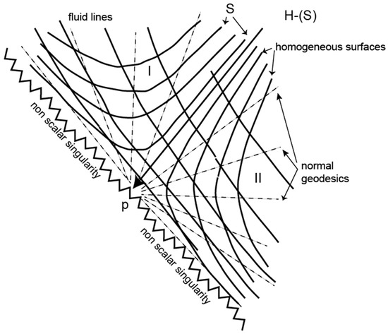
Figure 5.
Construction of a “whimper” singularity.
This null line is singular and corresponds to an intermediate singularity. Density and pressure are finite at any point arbitrarily close to the singularity; in fact, the limiting value of these quantities is precisely that which they take on the null surface H−(S), which is a homogeneous surface on which density and pressure are constant and perfectly defined.
Region I is spatially homogeneous (the homogeneity surfaces are spatial), while region II is stationary (the homogeneity surfaces are temporal).
Let us consider an observer moving towards the singularity along a geodesic orthogonal to the homogeneity surfaces in region I.
He measures a matter density = Tabnanb (na being the normal vector). Since homogeneous surfaces become spatial in region I after being temporal in region II, the normal vector na becomes null on H−(S), so the scalar product uana diverges on homogeneity surfaces tending towards H−(S) and p (ua is the fluid velocity). The stress–energy tensor of a perfect fluid has the following form:
Tab = (w + p)uaub + pgab; we see that = (w + p)(uana)2 − p becomes infinite as we approach p. Therefore, the observer moving towards p measures an infinite density of matter.
This situation is an exact analogue of what happens in four dimensions. The curvature tensor measured in an orthonormal frame of reference along an orthogonal geodesic ending at p diverges if the frame of reference is transported parallel; on the other hand, it is perfectly regular in another orthonormal frame of reference along the curve (for example, a tetrad with the 4-velocity of the fluid as the timelike vector).
The null homogeneous surface H−(S) is a prediction horizon or Cauchy horizon, in the sense that complete initial data on a spatially homogeneous surface S of region I completely determines the evolution of the field between S and H−(S), but not beyond.
An example of such a model is the “tilted” Bianchi type V universe found in [48], whose Penrose diagram has the shape shown in Figure 6.
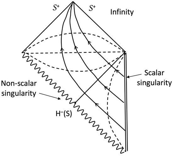
Figure 6.
Penrose diagram of a tilted Bianchi type V universe.
This example leads to the following question: is a non-scalar singularity always associated with a Cauchy horizon?
The answer is negative [37], although certain solutions which are globally hyperbolic (i.e., without a Cauchy horizon) and have non-scalar singularities provide a counter-example.
2.7. Existence of Non-Scalar Singularities
Let us list some very recent results relating to the occurrence of non-scalar singularities.
(a) Empty spaces of Petrov types III or N can only possess C0-non-scalar singularities (or locally extensible singularities), this being due to the fact that there is no C0-non-zero scalar invariant.
(b) There are vacuum solutions with C0-non-scalar singularities, in which the Petrov type is not constant in an open neighborhood of the singular point p. Consider for, example, a plane-wave solution in which the function A(u) is of class C− on (0, ∞) cancels on any interval (1/2n, 1/2n+1/2), where n is an integer, and is non-zero on any interval (1/2n+1/2, 1/2n+1) of maximum amplitude n2.
When n → ∞, A(u) oscillates indefinitely with Petrov types N and O. From (3) and (5), it is clear that we obtain a C0−-non scalar singularity.
(c) Empty spaces of Petrov types D, I, and II can have C0-non-scalar singularities but also C0-scalar singularities (unlike the other types, see above).
(d) All C0-non-scalar singularities (whether Weyl, Ricci, or mixed singularities) can be described as due to an irregular Lorentz transformation between a “good” tetrad and a parallely transported tetrad [49].
(e) In general, non-scalar singularities are both Weyl and Ricci singularities (Siklos, 1976) [49].
(f) A study of the possible behavior of the curvature tensor along a curve approaching a non-scalar singularity has been carried out by Ellis and Schmidt [37]; one of the conclusions is that C0-non-scalar singularities can occur in spaces with positive definite metrics, but C0−-non-scalar singularities cannot.
To conclude this section, let us mention that so far, there is no theorem relating to the “instability” of non-scalar singularities, in the sense that if a spatially homogeneous model possessing a non-scalar singularity is subjected to perturbations, the non-scalar singularity would transform into a scalar singularity. Indeed, if a photon were sent through the Cauchy horizon H−(S), there would be a spectral shift towards infinite blue as it approached the non-scalar singularity [47]. The photon would then arrive with infinite energy, and the effect of the perturbation would be to transform the non-scalar singularity into a scalar singularity. Work by Belinskii, Khalatnikov, and Lifshitz [50] and King [51] suggests that non-scalar singularities are indeed unstable because they would be linked to conditions of strong symmetry in spacetime, so that in general cosmological models (without symmetry), such a situation would not occur.
2.8. Scalar Singularities
In the notation of [19], scalar singularities are s.p.curvature singularities (“scalar polynomial”).
Ellis and King [47] showed that in a perfect fluid spacetime whose equation of state p = p(w) is such that the inequalities w + 3p ≥ 0, w + p > 0, 0 ≤ dp/dw ≤ 1 are verified, a “curvature singularity” appears on a given curve if and only if a scalar singularity appears there. The “curvature singularity” referred to here is defined according to the terminology of certain articles [20,47] such that the components of the curvature tensor measured in any orthonormal reference frame along the curve are divergent.
This type of singularity is both the best known and the closest to the intuitive physical conception of a singularity, as the following examples show.
(1) Friedmann–Lemaître Universe
These are solutions to Einstein’s equations that are spatially homogeneous and isotropic, with a perfect fluid. The metric can be written as follows:
where d∑2 is the metric of a 3-space of constant curvature k = +1, 0 or −1. The fluid moves at 4-velocity ua = δa0.
ds2 = −dt2 + R2(t)d∑2
We show that if w + 3p > 0 and w + p > 0, there is a scalar singularity at the beginning of each expansion phase: w → ∞ when t → 0, and the Ricci curvature invariant RabRab diverges
(2) Schwarzschild inner solution
The well-known metric is written as follows:
with 0 ≤ ϕ ≤ 2π, −∞ <t < ∞, 0 < r < 2m.
ds2 = −(1 − 2m/r)dt2 + (1 − 2m/r)−1dr2 + r2(sin2θ dϕ2 + dθ2)
r = 0 is a scalar singularity, because the conformal curvature invariant RabcdRabcd becomes infinite there.
(3) Orthogonal spatially homogeneous cosmologies
This applies to a perfect fluid whose universe lines are orthogonal to the homogeneous hypersurfaces or class A tilted cosmologies [39]. These models will be studied in detail in a second article.
(4) Stationary solutions with cylindrical symmetry and incoherent matter.
These spaces admit a three-parameter abelian group of isometries acting transitively on temporal hypersurfaces; the temporal Killing vector is tangent to these surfaces [52]. Some solutions, such as that of Maitra [53], are geodesically complete, while others have a Weyl singularity (the scalar Eabgab becomes infinite, where Eab is the “electric” part of the Weyl tensor), or an oscillatory Ricci singularity (the Ricci scalar polynomial RabRab is of the form 2sin2 (1/r) + f(r), where f is monotonic, and therefore has no limit when r tends to zero).
Presumably, the existence of scalar singularities is stable under small perturbations. Here, again, there is no definitive theorem, but there are strong presumptions [4,54].
Note that proving the existence of a scalar singularity is not always trivial. Despite Cauchy data that would formally lead to a scalar singularity, it is mathematically possible that the Cauchy development is precisely not the one expected; spacetime may, for example, ‘end’ before the predicted singularity occurs. We need to ensure that the predictions (or retrodictions) made on the basis of formally adequate Cauchy data are not distorted by the spontaneous appearance of ‘unexpected’ singularities (for example, a conformal singularity with infinite matter density). To achieve this, we postulate that spacetime is maximal and has no “holes”, i.e., that for any spatial surface S with no boundary, the dependence domain D(S) is such that there is no isometry Φ: D(S) → N in another spacetime N for which D(Φ(S)) ≠ Φ(D(S) [45].
For example, the universal cover of the Minkowski space amputated from the 2-plane (t = 0, x = 0) is maximal but has a hole; indeed, D({t = −1}) is “holed” by the singularity at t = x = 0, and its image under the natural application Φ which sends it into the Minkowski space is a proper subset of D(Φ({t = −1})), which is the entire space.
Using D instead of D+ makes the definition symmetric between prediction and backtracking, which avoids having to decide which time arrow to choose.
We will not dwell on the properties of scalar singularities here, as we will be studying their various structures in detail in a further article.
3. Occurrence of Singularities
3.1. Theorems
We will briefly deal with the part relating to the famous theorems on the occurrence of singularities in Cosmology; theorems which, with the discovery of the cosmic background radiation at 2.7 °K, were at the origin of a great revival of interest in singularities among cosmologists. As this subject has been remarkably and exhaustively dealt with in the classic book by Hawking and Ellis [19], we shall confine ourselves to listing these theorems without demonstration and discussing their conditions and fields of application.
We have already pointed out in Section 1.1 that some physicists in the 1960s regarded singularities in General Relativity simply as the result of symmetries imposed on spacetime. The most representative authors of this school, Lifshitz and Khalatnikov, published a series of works showing that certain classes of solutions with a “physical” singularity (infinite matter density or pressure) did not contain the number of arbitrary functions required to specify a general (i.e., symmetry-free) solution of Einstein’s equations [1]. The two authors then hypothesized that the Cauchy data giving rise to such singularities formed a subset of zero measure in the set of all Cauchy data and therefore did not occur in the real universe.
We have already seen that this hypothesis has in fact been invalidated by the proof of general theorems on the occurrence of singularities.
The first theorem not involving a symmetry assumption was formulated by Penrose [2] and demonstrates the occurrence of a singularity in a star undergoing gravitational collapse below its Schwarzschild radius.
However, the Schwarzschild surface is only defined for exact spherical symmetry. Penrose therefore introduced the more general concept of a closed trapped surface S, which is a compact, edgeless 2-space surface (whose topology is usually S2), such that the two families of geodesics (incoming and outgoing) orthogonal to S each converge on S.
The rigorous statement is as follows:
Theorem 1.
The spacetime (M, g) cannot be n-g-complete if all the following conditions are satisfied:
- (1)
- RabKaKb ≥ 0 for any null vector Ka
- (2)
- there exists a noncompact Cauchy surface in M
- (3)
- there exists a closed trapped surface S in M
Let us briefly discuss the conditions of the theorem.
Condition (1) holds, provided that the energy density is positive for any observer.
Condition (3) holds, at least in some region of spacetime (see Section 9 of [19]).
The relative “weakness” of the theorem lies in condition (2), which imposes the existence of a Cauchy surface, so the theorem does not predict the existence of singularities in physically realistic cosmological models. In fact, it shows that a gravitational collapse leads either to a singularity (more precisely, an n-g-incompleteness) or to a Cauchy horizon—either way, the prediction is broken.
A theorem by Hawking and Penrose [6] overcomes this difficulty:
Theorem 2.
(M, g) is c-g-complete if:
- (1)
- RabKaKb ≥ 0 for any null vector Ka
- (2)
- the generic condition is satisfied
- (3)
- M satisfies the causality condition
- (4)
- at least one of the following three conditions is satisfied:
- (4i)
- there exists an achronal compact set without edge
- (4ii)
- there is a closed trapped surface
- (4iii)
- there exists a point p such that on any null geodesic from p, the divergence θ becomes negative
This theorem is more general than the first. On the one hand, condition (1) corresponds to the weak energy condition, which involves not only zero vectors as in Theorem 1, but also time vectors; on the other hand, the existence of a closed occlusive surface is now only one of three possible conditions.
It can be shown that (4i) is satisfied in a spatially closed solution; (4iii) is satisfied if the reconverging light cone is our own light cone from the past (observation of radiation at 3 °K). The genericity condition (2) is written as KaKbK[cRd]ab[eKf] ≠ 0 for any causal geodesic with tangent unit vector Ka; it is reasonable in any physically realistic solution (p.101 of [19]).
However, Theorem 2 does not specify whether the singularities occur in the past or the future. If (4i) is verified, the singularity is in the future; if (4ii) is verified, nothing can be said; if (4iii) is verified, the singularity is in the past.
A theorem of Hawking [55] solves this question:
Theorem 3.
There exists an incomplete causal geodesic in the past passing through a given point p of spacetime M if:
- (1)
- RabKaKb ≥ 0 for any causal vector Ka
- (2)
- M satisfies the causality condition
- (3)
- At point p, there exists a temporal unit vector of the past W and a constant b > 0 such that if V is the unit vector tangent to the temporal geodesics of the past passing through p, on each of these geodesics, the expansion θ ≡ Va;a becomes less than −3c/b (where c = −WaWa) in the distance interval [0, b/c] measured from p along these geodesics.
Condition (3) simply means that the past-time geodesics from p reconverge within a compact region located in the past of p. This situation is illustrated in Figure 7.
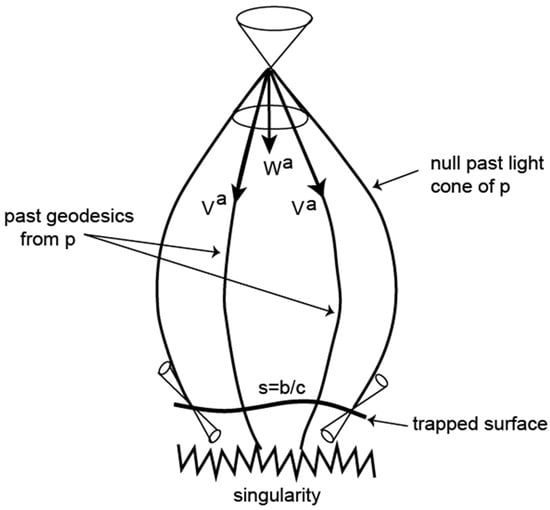
Figure 7.
Reconvergence of past-time geodesics within a trapped surface.
Theorems 2 and 3 are the most useful because their assumptions can be shown to be satisfied in a large number of solutions of the physically realistic Einstein equations.
Finally, these theorems involve the condition of causality, and one could envisage a violation of causality rather than an incompleteness of spacetime. A theorem by Hawking (1967) [27] shows that this is not the case:
Theorem 4.
Spacetime is t-g-incomplete if:
- (1)
- RabKaKb ≥ 0 for any causal vector Ka
- (2)
- there exists a compact 3-edgeless space surface S
- (3)
- the unit normals to S are everywhere divergent (or everywhere convergent) on S
Here, (1) is the weak energy condition; (2) refers to the closure of the universe; (3) is interpreted as saying that the universe is expanding (or contracting).
Geroch [56] also contributed to these questions with a theorem close in substance to Theorem 4.
3.2. Conclusions
As we have seen, these extremely important theorems prove, within the framework of General Relativity and under reasonable physical hypotheses, the existence of a singularity in the past of the universe or a singularity in the future as far as the gravitational collapse of stars is concerned.
In fact, they simply tell us that spacetime has incomplete causal geodesics. These incomplete geodesics define singular points on the b-boundary ∂M, but we know nothing about the physical nature of these singularities.
In an attempt to elucidate this fundamental question, several directions are open to the researcher, which remain relevant today. Among them:
(a) The Penrose–Hawking singularity theorems prove the inevitability of spacetime singularities in general relativity under classical and rather reasonable conditions, but they say very little about their nature [57]. “Weak” singularities in which all the scalar quantities remain finite can occur in the so-called tilted Bianchi cosmologies. However, such cosmological models are likely not generic. Belinskii, Khalatnikov, and Lifshitz [58,59]–hererafter BKL–have conjectured that for a generic inhomogeneous relativistic cosmology, the approach to the spacelike singularity into the past is vacuum dominated and oscillatory, obeying the so-called BKL or mixmaster dynamics—for a synthesis, see [60]. Numerical simulations have been used, e.g., [61,62], to verify the BKL dynamics in special classes of spacetimes. Rigorous mathematical results on the dynamical behavior of Bianchi type VIII and IX cosmological models have also been presented in [63]. The interest in considering generic solutions is that the behavior of a general solution (without symmetry) in the vicinity of a singularity can be considered qualitatively similar to the behavior of these particular generic solutions. In a second part of the present review on spacetime singularities, we shall discuss the oscillatory approach to singularities in Bianchi-type cosmological models.
(b) We can try to weave the link between the singularities predicted by General Relativity and those studied in other branches of physics. In this respect, René Thom’s theory of catastrophes [64] could provide some interesting results, but as far as I know, this method has not been developed. However, while catastrophe theory remains largely unexplored in this context, dynamical systems techniques, like phase space and stability analysis, have provided powerful tools for studying the evolution and classification of singularities, especially in relation to BKL dynamics, see, e.g., [65,66].
(c) We could also consider the “brutal” method of numerically integrating Einstein’s equations on a computer. Full 3D simulations of Einstein’s field equations became possible only with the advent of supercomputers and robust numerical relativity formalisms in the 1990s and early 2000s, see e.g., [67]. They have become essential for exploring dynamical spacetime evolution, shedding light on black hole interiors, gravitational collapse, and phenomena like critical behavior—e.g., [68]. More recent work addresses mass inflation, weak singularities, and Cauchy horizon stability, e.g., [69].
(d) In order to sketch a bridge to current work in the study of singularities, it is useful to recall that much of the mystery of singularities hinges on a unified theory of quantum gravity, which could provide a deeper understanding of these exotic objects. The term “soft singularities” has become more prevalent in recent years, particularly in the context of black hole physics and quantum gravity. It is used to describe singularities where the breakdown of spacetime geometry is “milder” or less extreme than what we typically expect from classical singularities, like those associated with black holes or the Big Bang. They arise in various contexts, including string theory and fuzzball models [70], quantum cosmology and quantum bounce [71], black hole evaporation [72], soft hair models [73], and quantum gravity models that smooth the infinite curvatures of traditional singularities [74]. While the exact nature and mathematical formulation of soft singularities remain an open area of research, they are part of an effort to understand and resolve the infinities predicted by classical general relativity through quantum mechanical effects.
Funding
This research received no external funding.
Acknowledgments
The author thanks the anonymous referees for their helpful comments, which improved the quality of the manuscript.
Conflicts of Interest
The author declares no conflict of interest.
References
- Lifshitz, E.M.; Khalatnikov, I.M. Investigations in relativistic cosmology. Adv. Phys. 1963, 12, 18. [Google Scholar] [CrossRef]
- Penrose, R. Gravitational Collapse and space-time singularities. Phys. Rev. Lett. 1965, 14, 57. [Google Scholar] [CrossRef]
- Hawking, S.W. The occurrence of singularities in Cosmology. Proc. Roy. Soc. Lond. A 1966, 294, 511–521. [Google Scholar]
- Lifshitz, E.M.; Khalatnikov, I.M. Oscillatory approach to singular point in the open cosmological model. JETP Lett. 1970, 11, 123. [Google Scholar]
- Brans, C.; Dicke, R.H. Mach’s Principle and a Relativistic Theory of Gravitation. Phys. Rev. 1961, 124, 925. [Google Scholar] [CrossRef]
- Hawking, S.W.; Penrose, R. The singularities of gravitational collapse and Cosmology. Proc. R. Soc. Lond. Ser. A Math. Phys. Sci. 1970, 314, 529–548. [Google Scholar]
- Hehl, F.W.; von der Heyde, P.; Kerlick, G.F.; Nester, J.M. General relativity with spin and torsion: Foundations and Prospects. Rev. Mod. Phys. 1976, 48, 393–416. [Google Scholar] [CrossRef]
- Penrose, R. Gravitational Collapse: The Role of General Relativity. Nuovo C. Riv. Ser. 1969, 1, 252. [Google Scholar]
- Christodolou, D. Violation of cosmic censorship in the gravitational collapse of a dust cloud. Comm. Math. Phys. 1984, 93, 171–195. [Google Scholar] [CrossRef]
- Christodolou, D. The instability of naked singularities in the gravitational collapse of a scalar field. Ann. Math. 1999, 149, 183–217. [Google Scholar] [CrossRef]
- Dafermos, M. Black holes without spacelike singularities. Commun. Math. Phys. 2014, 332, 729–757. [Google Scholar] [CrossRef]
- Landsman, K. Singularities, black holes and cosmic censorship: A tribute to Roger Penrose. arXiv 2021, arXiv:2101.02687. [Google Scholar] [CrossRef]
- Van de Moortel, M. The Strong Cosmic Censorship Conjecture. Comptes Rendus. Mécanique 2025, 353, 415–454. [Google Scholar] [CrossRef]
- Hawking, S.W. Breakdown of Predictability in Gravitational Collapse. Phys. Rev. D 1976, 14, 2460–2473. [Google Scholar] [CrossRef]
- Crowther, K.; De Haro, S. Four Attitudes Towards Singularities in the Search for a Theory of Quantum Gravity. In The Foundations of Spacetime Physics: Philosophical Perspectives; Vassallo, A., Ed.; Routledge: New York, NY, USA, 2022; pp. 223–250. [Google Scholar]
- Joshi, P.S. Spacetime Singularities. In Springer Handbook of Spacetime; Ashtekar, A., Petkov, V., Eds.; Springer: Berlin/Heidelberg, Germany, 2014; pp. 409–436. [Google Scholar]
- Curiel, E. Singularities and Black Hole. In The Stanford Encyclopedia of Philosophy; Zalta, E., Ed.; Springer: Berlin/Heidelberg, Germany, 2019; Available online: https://plato.stanford.edu/ (accessed on 22 July 2025).
- Schmidt, B.G. A new definition of singular points in General Relativity. Gen. Relativ. Gravit. 1971, 1, 269–280. [Google Scholar] [CrossRef]
- Hawking, S.W.; Ellis, G.F.R. The Large Scale Structure of Space-Time; Cambridge University Press: Cambridge, UK, 1973. [Google Scholar]
- Clarke, C.J.S. Singularities in Globally Hyperbolic Space-Times. Commun. Math. Phys. 1975, 41, 65. [Google Scholar] [CrossRef]
- Sobolev, S.L. Applications of Functional Analysis in Mathematical Physics; American Mathematical Society: Providence, RI, USA, 1963. [Google Scholar]
- Misner, C.W.; Thorne, K.S.; Wheeler, J.A. Gravitation; Freeman: San Francisco, CA, USA, 1974. [Google Scholar]
- Choquet-Bruhat, Y. Espace-temps einsteiniens généraux et chocs gravitationneIs. Ann. l’I.H.P. Phys. Théorique 1968, 8, 327–338. [Google Scholar]
- Kobayashi, S.; Nomizu, K. Foundations of Differential Geometry; Interscience: New York, NY, USA; London, UK, 1963. [Google Scholar]
- Kundt, W. Note on the completeness of space-times. Z. Für Phys. 1963, 172, 488. [Google Scholar] [CrossRef]
- Geroch, R.P. What is a singularity in General Relativity? Ann. Phys. 1968, 48, 526. [Google Scholar] [CrossRef]
- Hawking, S.W. The occurrence of singularities in Cosmology III. Causality and singularities. Proc. Roy. Soc. Lond. A 1967, 300, 187. [Google Scholar]
- Geroch, R.P. Singularities in closed universes. Phys. Rev. Lett. 1966, 17, 445. [Google Scholar] [CrossRef]
- Geroch, R.P. Local characterization of singularities in General Relativity. J. Math. Phys. 1968, 9, 450. [Google Scholar] [CrossRef]
- Geroch, R.P.; Kronheimer, E.; Penrose, R. Ideal points in space-time. Proc. Roy. Soc. Lond. A 1972, 327, 545. [Google Scholar]
- Seifert, H.J. The causal structure of singularities. In Proceedings of the Conference on Differential Geometrical Methods in Mathematical Physics, Bonn, Germany, 1–4 July 1975; pp. 539–565. [Google Scholar]
- Schmidt, B.G. Local completeness of the b-boundary. Commun. Math. Phys. 1972, 29, 49. [Google Scholar] [CrossRef]
- Steenrod, N. The Topology of Fibre Bundles; Princeton University Press: Princeton, NJ, USA, 1951. [Google Scholar]
- Friedrich, H. Construction and properties of space-time b-boundaries. Gen. Rel. Grav. 1974, 5, 681. [Google Scholar] [CrossRef]
- Clarke, C.J.S. Local extensions in Singular Space-Times. Commun. Math. Phys. 1973, 32, 205. [Google Scholar] [CrossRef]
- Clarke, C.J.S. The Classification of Singularities. Gen. Rel. Grav. 1975, 6, 35. [Google Scholar] [CrossRef]
- Ellis, G.F.R.; Schmidt, B.C. Singular Spacetimes. Gen. Rel. Grav. 1977, 8, 915–953. [Google Scholar] [CrossRef]
- Kruskal, M.P. Maximal extension of Schwarzschild metric. Phys. Rev. 1960, 119, 1743. [Google Scholar] [CrossRef]
- King, A.R.; Ellis, G.F.R. Tilted homogeneous cosmological models. Commun. Math. Phys. 1973, 31, 209. [Google Scholar] [CrossRef]
- Ryan, M.P.; Shepley, L.C. Homogeneous Relativistic Cosmologies; Princeton University Press: Princeton, NJ, USA, 1975. [Google Scholar]
- Newman, E.T.; Tamburino, L.; Unti, T.J. Empty space generalization of the Schwarzschild metric. J. Math. Phys. 1963, 4, 915. [Google Scholar] [CrossRef]
- Misner, C.W.; Taub, A.H. A singularity-free empty universe. Sov. Phys. JETP 1969, 28, 122. [Google Scholar]
- Misner, C.W. Taub-NUT space as a counterexample to almost anything. In Relativity & Cosmology; Ehlers, J., Ed.; Lectures in Applied Mathematics; Providence: Providence, RI, USA, 1967; Volume 8, p. 160. [Google Scholar]
- Clarke, C.J.S. Space-Time Singularities. Commun. Math. Phys. 1976, 49, 17. [Google Scholar] [CrossRef]
- Ehlers, J.; Kundt, W. Exact solutions of the gravitational field equations. In Gravitation: An Introduction to Current Reasarch; Witten, L., Ed.; John Wiley & Sons: Hoboken, NJ, USA, 1962. [Google Scholar]
- Ellis, G.F.R. Relativistic Cosmology. In General Relativity and Cosmology; Sachs, R., Ed.; Academic Press: Cambridge, MA, USA, 1971. [Google Scholar]
- Ellis, G.F.R.; King, A.R. Was the big-bang a whimper? Commun. Math. Phys. 1974, 38, 119. [Google Scholar] [CrossRef]
- Farnsworth, D.L. Some New General Relativistic Dust Metrics possessing Isometries. J. Math. Phys. 1967, 8, 2315–2317. [Google Scholar] [CrossRef]
- Siklos, S. Two completely singularity-free nut spacetimes. Phys. Lett. A 1976, 59, 173–174. [Google Scholar] [CrossRef]
- Belinskii, V.A.; Lifshitz, E.M.; Khalatnikov, I.M. Construction of a General Cosmological Solution of the Einstein Equations with a time Singularity. Sov. Phys. JETP 1972, 35, 838. [Google Scholar]
- King, A.R. Instability of Intermediate singularities in, general relativity. Phys. Rev. D 1975, 11, 763. [Google Scholar] [CrossRef]
- King, A.R. New Types of Singularity in General Relativity. Commun. Math. Phys. 1974, 38, 157. [Google Scholar] [CrossRef]
- Maitra, S.C. Stationary Dust-Filled Cosmological Solution with Λ=0 and without Closed Timelike Lines. J. Math. Phys. 1966, 7, 1025. [Google Scholar] [CrossRef]
- Eardley, D.M.; Liang, K.; Sachs, K. Velocity-dominated singularities in irrotational dust cosmologies. J. Math. Phys. 1972, 13, 99. [Google Scholar] [CrossRef]
- Hawking, S.W. On the rotation of the universe. Mon. Not. R. Astron. Soc. 1969, 142, 129. [Google Scholar] [CrossRef]
- Geroch, R.P. Singularities. In Relativity; Carmeli, M., Fickler, S., Witten, L., Eds.; Plenum Press: New York, NY, USA, 1970; pp. 259–291. [Google Scholar]
- Senovilla, J.M.M. Singularity theorems in general relativity: Achievements and open questions. In Einstein and the Changing Worldviews of Physics, Chapter 15; Lehner, C., Renn, J., Schemmel, M., Eds.; Einstein Studies 12; Birkhäuser: Boston, MA, USA, 2012. [Google Scholar]
- Belinskii, V.A.; Khalatnikov, I.M.; Lifschitz, E.M. Oscillatory Approach to a Singular Point in the Relativistic Cosmology. Adv. Phys. 1970, 19, 525–573. [Google Scholar] [CrossRef]
- Belinskii, V.A.; Khalatnikov, I.M.; Lifschitz, E.M. A general solution of the Einstein equations with a time singularity. Adv. Phys. 1982, 31, 639–667. [Google Scholar] [CrossRef]
- Belinskii, V.A.; Henneaux, M. The Cosmological Singularity; Cambridge University Press: Cambridge, UK, 2015. [Google Scholar]
- Berger, B.K. Numerical Approaches to Spacetime Singularities. Living Rev. Relativ. 2002, 5, 1. [Google Scholar] [CrossRef] [PubMed]
- Garfinkel, D. Numerical relativity beyond astrophysics. Rep. Progr. Phys. 2017, 80, 016901. [Google Scholar] [CrossRef] [PubMed]
- Brehm, B. Bianchi VIII and IX vacuum cosmologies: Almost every solution forms particle horizons and converges to the Mixmaster attractor. arXiv 2016, arXiv:1606.08058. [Google Scholar] [CrossRef]
- Thom, R. Stabilité Structurelle et Morphogénèse; Benjamin: New York, NY, USA, 1969. [Google Scholar]
- Bahamonde, S.; Boehmer, C.G.; Carloni, S.; Copeland, E.J.; Fang, W.; Tamanini, N. Dynamical systems applied to cosmology: Dark energy and modified gravity. Phys. Rep. 2018, 775–777, 1–122. [Google Scholar] [CrossRef]
- Roy, B.C.; Chanda, A.; Paul, B.C. Dynamical stability and phase space analysis of an Emergent Universe with non-interacting and interacting fluids. arXiv 2024, arXiv:2401.00782. [Google Scholar] [CrossRef]
- Baumgarte, T.; Shapiro, S. Numerical integration of Einstein’s field equations. Phys. Rev. D 1998, 59, 024007. [Google Scholar] [CrossRef]
- Choptuik, M.W. Universality and scaling in gravitational collapse of a massless scalar field. Phys. Rev. Lett. 1993, 70, 9–12. [Google Scholar] [CrossRef] [PubMed]
- Hod, S.; Piran, T. Mass-Inflation in Dynamical Gravitational Collapse of a Charged Scalar-Field. Phys. Rev. Lett. 1998, 81, 1554–1557. [Google Scholar] [CrossRef]
- Mathur, S.D. String theory and Black hole Fuzzballs: A brief review. Int. J. Mod. Phys. A 2005, 20, 2009–2028. [Google Scholar]
- Ashtekar, A.; Singh, P. Loop quantum cosmology: A status report Class. Quantum Gravity 2011, 28, 213001. [Google Scholar] [CrossRef]
- Bañados, M.; Cano, P.A. The final state of a black hole: Thermal or singular? J. High Energy Phys. 2015, 2015, 1–10. [Google Scholar]
- Hawking, S.W.; Perry, M.J.; Strominger, A. Soft Hair on Black Holes. Phys. Rev. Lett. 2016, 116, 231301. [Google Scholar] [CrossRef]
- Giddings, S.B.; Karczmarek, J. A new approach to black holes and cosmology in the AdS/CFT context. Phys. Rev. D 2009, 80, 065011. [Google Scholar]


Disclaimer/Publisher’s Note: The statements, opinions and data contained in all publications are solely those of the individual author(s) and contributor(s) and not of MDPI and/or the editor(s). MDPI and/or the editor(s) disclaim responsibility for any injury to people or property resulting from any ideas, methods, instructions or products referred to in the content. |
© 2025 by the author. Licensee MDPI, Basel, Switzerland. This article is an open access article distributed under the terms and conditions of the Creative Commons Attribution (CC BY) license (https://creativecommons.org/licenses/by/4.0/).