Abstract
I show here that if we construct D-branes not in the form of infinite superpositions of string modes, in order to satisfy the technical condition of coherence by means of eigenstates of annihilation operators, but instead insist on an approximate but much more physical and practical definition based on phase coherence, we obtain finite (and hence realistic) superpositions of string modes that would form realistic D-branes that would encode (at least as a semiclassical approximation) various quantum properties. Re-deriving the AdS/CFT duality by starting in the pre-Maldacena limit from such realistic D-branes would lead to quantum properties on the AdS side of the duality. Causal structures can be modified in various many-particle systems, including strings, D-branes, photons, or spins; however, there is a distinction between the emergence of an effective causal structure in the inner degrees of freedom of a material, in the form of a correlation-generated effective metric, for example, in a spin liquid system, and the emergence of a causal structure in an open propagating system by using classical light. I will show how an Uhlmann gauge construction would add stability to a modified causal structure that would retain the shape of a closed causal loop. Various other ideas related to the quantum origin of the string length are also discussed and an analogy of the emergence of string length from quantum correlations with the emergence of wavelength of an electromagnetic wave from coherence conditions of photon modes is presented.
1. Introduction
The AdS/CFT correspondence [1] emerges naturally from string theory as a specific realisation of the general open–closed string duality [2]. This duality refers to the equivalence between two seemingly different descriptions of string interactions: the open string channel, describing strings with endpoints attached to D-branes that interact forming loop diagrams of open strings attached to boundaries, and the closed string channel, in which the same physical process can equivalently be described by closed strings propagating freely without endpoints, exchanged between D-branes, and forming cylindrical diagrams. Formally, this duality is expressed as an equality between two conformal field theory amplitudes
Here, and are modular parameters related by a conformal transformation, essentially exchanging time and space coordinates in the string worldsheet. This relationship is fundamental and mathematically rigorous, arising naturally from modular invariance of the string worldsheet partition function. The validity of the open–closed duality is rooted in the structure of two-dimensional conformal field theory and the geometry of string theory. String theory amplitudes are integrals over the moduli space of Riemann surfaces. Modular transformations map one amplitude with boundary (open strings) to amplitudes without boundary (closed strings). This ensures the mathematical equivalence between open and closed string descriptions. From a worldsheet perspective, consider a cylindrical worldsheet. In the open string channel the cylinder has boundaries (representing D-branes) and in the closed string channel the cylinder has no boundaries, as it is viewed as a propagation of closed strings. Modular transformation maps one interpretation (boundaries) to the other (no boundaries), preserving the physics. In short, the reason the open–closed duality holds is due to the underlying symmetries (modular invariance) and consistency conditions (unitarity and locality) of the string theory itself [3]. The AdS/CFT correspondence emerges naturally from the physics of D-branes in string theory [4]. Consider a stack of N coincident D3-branes embedded in Type IIB superstring theory. In the open string description, the dynamics of open strings with endpoints attached to the D3-branes generates a low-energy theory of the brane worldvolume. At low energies, open strings attached to N D3-branes yield a gauge theory
In a closed string description, the strings propagate in the bulk, influenced by the mass energy of the D-branes. At large N and strong coupling, the geometry created by these branes can be described by supergravity, a low effective theory of closed strings. The near horizon geometry around the D3-branes is precisely
Taking the low-energy limit (decoupling limit) isolates the physics on the D-branes from the asymptotically flat region. On the open string side (boundary theory) decoupling the gravitational interactions, the open string description becomes purely the boundary gauge theory
On the closed string side (the bulk theory) near the horizon of the D3-branes, the closed string description simplifies to the supergravity low-energy limit of closed strings on
Thus, we have two entirely equivalent descriptions of the same physical system: a gauge theory living on the boundary (open string origin) and a gravitational theory living in the bulk (closed string origin). The equivalence is precisely the AdS/CFT correspondence
AdS/CFT is essentially a concrete manifestation of open–closed string duality [5]. Open string diagrams on D-branes can equivalently be described as closed string diagrams exchanged between branes [6]. In the special limit where D-branes are numerous (), their gravitational backreaction produces a well-defined closed string geometry (). From a holographic standpoint, the open string degrees of freedom on the brane correspond to closed string gravitational dynamics in the bulk geometry. The branes become the boundary on which the CFT lives, while closed strings are the bulk degrees of freedom. This clearly shows why is obtained precisely from the open–closed duality: it is nothing more than the realisation of this duality at large N and strong coupling [7,8]. The black brane interior, however, is not covered by the AdS/CFT duality [7]. Initially, the AdS/CFT correspondence has been stated as a duality between the bulk gravitational theory (closed string picture), usually classical supergravity or quantum gravity on an asymptotically AdS spacetime, and a boundary conformal field theory (open string picture), a non-gravitational quantum field theory defined on the boundary of AdS. The boundary theory lives at the spatial boundary (at infinity) of AdS spacetime. Thus, strictly speaking the duality directly encodes information accessible at or near the boundary and any event or phenomenon deep inside a black hole appears at first to be beyond direct boundary reach. The naive holographic dictionary maps bulk fields near the boundary onto boundary operators, making it unclear how it directly describes the interior of the black hole. However, even though the AdS/CFT duality does not give an obvious dictionary mapping boundary operators directly to fields inside the black hole interior, it provides indirect methods to study the interior. Some of these are analytic continuations of boundary observables, quantum entanglement and entanglement wedges, reconstruction techniques a la HKLL reconstruction [9] or bulk operator reconstruction [10], state-dependent operators [11], complexity considerations, etc. In general, the black hole’s interior is also encoded because the AdS/CFT is a non-local quantum holographic duality [12]. What seems like a spatially inaccessible region due to a classical causal structure becomes accessible when we notice that the duality maps entanglement and quantum information in a fundamentally non-local way. The boundary observables contain subtle quantum interference patterns, correlations, and entanglement structures that encode events behind the horizon. Although classical causality prevents still direct access, quantum correlations, like entanglement or complexity-based reconstructions, provide indirect access to interior physics. In AdS/CFT, the gauge theory lives very near the horizon of a black brane and is formed by the N D-branes linked by open strings. The bulk is the physics close to the horizon, described by classical gravity, hence closed strings, forming the AdS space, on the outside of the horizon. The bulk is then the region outside the horizon, farther away from the boundary where the gauge theory lives. Initially, when we derive the AdS/CFT correspondence starting from string theory and D-branes; gauge theory is a boundary theory originating from open strings attached directly to the stack of N D3-branes. In the low-energy limit, these open strings form a non-gravitational gauge theory ( SYM) that lives on the world volume of the branes. When taking the low-energy decoupling limit, the gauge theory effectively resides at the boundary at infinity of the emergent gravitational geometry, namely at the conformal boundary of the emergent AdS spacetime. For the closed strings (in the bulk theory) originally, the closed strings propagated everywhere, including near the branes. However, when we have a large number of branes () and consider strong coupling, the branes’ gravitational backreaction creates a non-trivial curved spacetime. In particular, close to the horizon, but still outside it, we will obtain the geometry we expected
Thus, the bulk in the standard AdS/CFT dictionary refers usually to this gravitational region near (but outside) the black brane horizon, extending all the way outwards to the boundary at infinity. This is the bulk from the viewpoint of AdS/CFT as usually presented. If, however, various methods for probing the inside of the black hole are employed, we can generalise and extend the meaning of the bulk. We can consider a two-sided eternal black AdS hole. In that case, the black hole is dual to two entangled copies of the CFT (a thermofield double state). In this case, we would have an extended Penrose diagram. Here, the black hole interior is accessible via analytic continuation and entanglement wedge reconstruction, even though it lies technically behind event horizons. By definition, in this context the bulk is “extended” to mean also the interior, since it is part of the complete spacetime that emerges from quantum entanglement between boundary CFTs. Even in one-sided black holes formed by collapse, it is possible to reconstruct operators inside the horizon by using non-local, state-dependent boundary operators. Therefore, the notion of bulk is extended to mean that interior as well. Let us now describe Maldacena’s limit in this context. Initially, in string theory setups we start with N D3-branes placed in flat 10-dimensional spacetime. On the open strings side, the endpoints live directly on these D-branes, defining a gauge theory (e.g., ) on the brane world volume itself. At this initial stage, the gauge theory clearly lives exactly where the D-branes are located. There is also no notion of a boundary at infinity yet. When we have many more D-branes (N becomes large) that are stacked together, they strongly deform the spacetime geometry due to their collective gravitational attraction. The metric produced by a stack of N D3-branes is given by
This geometry has a characteristic scale set by
When we take the low-energy decoupling limit (Maldacena limit) defined by sending (string length scale to zero) while keeping the energies fixed from the viewpoint of open strings on the branes, two crucial things happen. First, the open strings (the gauge theory side) stay confined exactly on the branes as they effectively decouple from gravity at infinity and form a purely field theoretic theory living precisely where the branes were placed originally (in the original coordinates, this is just flat space). Second, the closed strings (gravity side) will experience an infinitely strong “zoom-in” close to the horizon of the original D3-brane geometry. In other words, we are looking closer and closer to the region right near the brane’s horizon. Because we are zooming infinitely close to the brane, the horizon region expands by a very large amount. This near horizon region takes the form . This zooming-in near the horizon transforms the geometry from a brane localised in flat spacetime to an extended AdS space which now has a clear boundary at infinity. Before taking the limit, the branes are localised objects in flat space. After taking the limit, the near horizon region is stretched infinitely, creating a whole new geometry with an explicit boundary at infinity. The position of the gauge theory is coordinate-dependent. In the original coordinates (flat embedding), gauge theory was localised exactly on the brane. In the near horizon coordinates, the region originally containing the brane (the original horizon of the brane) now appears infinitely far away, it becomes precisely the boundary at infinity of AdS. In other words, the brane location when viewed from inside the near horizon geometry is no longer close by. It moves to the conformal boundary of AdS. This is because the decoupling limit zooms infinitely into the region near the brane, stretching what used to be a finite location into an infinitely distant boundary. Finally, another aspect of the common language used in holography needs to be somehow clarified. When we hear in the literature that we go “deep inside the bulk”, sometimes this is referred to as the “quantum gravity limit”; however, the AdS boundary is the high energy (UV regime of the gauge theory), while deeper inside the bulk we find the low-energy physics (IR regime of the gauge theory). In this context, “deep inside the bulk” means going towards the interior of the AdS spacetime away from the boundary at infinity. One should notice that the AdS geometry itself arises strictly in the near-horizon limit, which eliminates the original asymptotically flat region (Minkowski spacetime) where the D-branes originally lived. In fact, the true full geometry originally was not just AdS, it was an interpolating geometry, going from flat Minkowski spacetime far from branes to AdS very close to the branes. Therefore, quantum gravity, in a more fundamental sense (stringy effects, finite N corrections, gravitational quantum fluctuations, etc.) actually become relevant precisely in the regime where the Maldacena limit is no longer exact, i.e., precisely in the transitional region (near the original brane horizon), not strictly inside the AdS bulk geometry itself. The quantum gravitational phenomena are not really “deep inside AdS” but rather occur exactly in the domain where the original Maldacena limit is incomplete or starts to fail. Deep inside the bulk in the usual AdS/CFT terminology actually means going towards the classical IR gravitational regime, well described by classical (or semiclassical) gravity. Far from being “more quantum”, this region is often less quantum, precisely because it is described by classical supergravity. True quantum gravitational effects lie precisely outside this simplified classical description in the region connecting classical AdS to flat Minkowski space, or near the UV boundary itself, where strongly quantum effects (such as stringy or brane excitations, finite N corrections, Planckian effects) become inevitable. With this clarified, let us have a look at the relationship between background space (target space), the D-branes moving within it, and the worldsheet dynamics of strings. The target space is the spacetime manifold in which strings propagate. Initially, in the original D-brane construction we used to derive AdS/CFT, this target space is usually taken to be a simple flat Minkowski spacetime (10-dimensional Minkowski, e.g., type IIB superstring theory). D-branes themselves are extended objects occupying submanifolds of the target space. A D3-brane occupies a (3 + 1)-dimensional submanifold of the original 10-dimensional spacetime. A completely separate 2-dimensional space (the sheet swept out by the string as it evolves in time) whose dynamics is described by a 2-dimensional conformal field theory is embedded in the target space and has its own dynamics. Strings propagating in target space correspond to fields defined on this worldsheet. This is the intrinsic space of string motion, and fields on the worldsheet encode positions of the string in target space. Let us start with a flat Minkowski space. Adding D-branes will change this. Many D-branes together carry energy and charge and thus by Einstein’s equations (or supergravity equations) of motion, they curve spacetime around them. D-branes do not merely move in a fixed flat spacetime. They produce and respond to gravitational fields curving spacetime. Explicitly, for N D3-branes in type IIB string theory, the solution to supergravity equations gives a geometry
This is precisely the geometry describing the target-space curvature created by the stack of D3-branes. The Maldacena limit (, with energies scaled accordingly) focuses on the region close to the branes (small r). Here, the “1” in the drops out, leaving just the geometry explicitly
which is exactly the target space in the Maldacena limit. Before taking the limit, the D-branes are explicitly present at a finite location (at ). After taking the limit, the Maldacena limit zooms infinitely close to the branes. The original position of the branes moves to the boundary at infinity of AdS. After the limit, the explicit branes vanish from the new geometry, leaving behind only the curved AdS geometry they created. The gauge theory originally defined by open strings attached on the branes now lives exactly on this boundary at infinity. Thus, after the Maldacena limit, you no longer see explicit D-branes in the bulk. They appear only as boundary conditions at infinity encoding the gauge theory on the AdS boundary. The fundamental starting point of string theory is that dynamics of fields on the 2D worldsheet of the string are equivalent to strings propagating through a target space geometry. From the worldsheet perspective, we have a 2-dimensional CFT. The fields on this CFT are interpreted as embedding functions describing the string position in target space. From a background perspective, the target space geometry itself (metric, fields, curvature) appears as coupling constants in this 2D CFT. The fundamental duality at the heart of string theory is the duality between 2D conformal theory on the worldsheet and the target space geometry and fields. Now, specialising to AdS/CFT, in the original setup, we had open strings attached to D-branes which created gauge theory dynamics. From the worldsheet viewpoint, open string endpoints are restricted by boundary conditions given by D-branes. The worldsheet CFT describes open string modes whose low energy effective theory is gauge theory. From the target space point of view before taking the limit, the closed string geometry curved by D-branes approaches AdS near the branes. In the AdS/CFT limit, the near horizon region transforms into the AdS geometry. Open string gauge theory lives at the boundary and closed strings propagate in the bulk AdS geometry. Therefore, the AdS/CFT emerges from a specialised case of the general background worldsheet duality, namely that worldsheet CFT for open strings on D-branes results in a boundary gauge theory (open string sector) whereas closed string worldsheet CFT in curved geometry results in a gravitational AdS bulk (closed string sector). Thus, in AdS/CFT the general background worldsheet correspondence splits into open and closed sectors becoming precisely the open–closed duality. Open strings attached to D-branes result in the boundary gauge theory whereas closed strings in the curved geometry produced by D-branes becomes the bulk gravitational theory. In string theory the term “closed string geometry” generally means the spacetime geometry (target space) in which closed strings propagate. This geometry includes a metric and fields like the antisymmetric field, the dilaton and other possible fields. These fields and the metric are backgrounds that appear in the worldsheet sigma model describing closed string propagation. Closed string geometry is dynamically determined from the string theory equations of motion in the form of consistency conditions. Starting with a sigma model describing strings moving in a general target space geometry we have
Quantum consistency (conformal invariance at the quantum level) of this sigma model imposes conditions on the allowed target space geometries. These conditions become Einstein-type equations (supergravity equations) at low energy, typically
The solutions of these equations define consistent closed string backgrounds. The worldsheet–target space duality (often called just T-duality, although this is of course just one special case for the real worldsheet–target duality) refers to a symmetry in string theory that tells us that transformations of the geometry of the target spacetime leave the physics described by the worldsheet theory completely invariant. This duality is fundamental because it reveals an equivalence between seemingly different spacetime backgrounds when viewed from the perspective of the 2-dimensional string worldsheet. As mentioned earlier, in string theory we have two distinct perspectives. On the one side we have the worldsheet viewpoint in which the fundamental theory is a 2-dimensional quantum conformal field theory living on the worldsheet. This CFT describes fields which represent the embedding coordinates of the string in some higher dimensional target spacetime. On the other side we have the target space viewpoint. The spacetime geometry emerges as the background fields (metric , antisymmetric tensor field , dilaton , etc.) in the sigma model action of the worldsheet theory
Worldsheet–target space duality means that two apparently distinct sets of target space fields can correspond to exactly the same physics on the string worldsheet. Thus, the physics is invariant under certain transformations of the target space geometry. This duality emerges from the following mathematical property of 2-dimensional quantum field theories. First, the conformal invariance and the modular invariance. String worldsheet theories must be conformally invariant (scale-invariant and invariant under conformal transformations), ensuring consistent quantisation. This invariance strongly restricts possible backgrounds. Second, Buscher rules and gauging sigma-model isometries. If we consider a sigma model with an isometry (a symmetry of the target space metric, like translation symmetry in one direction) then we can gauge this symmetry by introducing gauge fields on the worldsheet, and then integrate out these gauge fields to obtain a new sigma model which looks different (has new metric and B-field), but because this process is exact at the quantum worldsheet level, the original and the new sigma models are physically equivalent. These transformations are called Buscher transformations and they precisely implement what we call T-duality. As an explicit example, a string moving on a circle of radius R is physically identical to a string moving on a circle of radius . This is the simplest explicit realisation of worldsheet–target space duality. Two distinct target spaces: circles with radius R and radius are physically identical from the viewpoint of string theory. Such a duality exists because strings, unlike particles, have finite extensions and thus probe geometry differently. A particle probes only points. But strings probe extended regions. Thus, two different geometries (e.g., small and large circles) can appear as identical if viewed from a string’s perspective, due to the interplay between momentum and winding modes. The momentum modes correspond to standard kinetic energy, sensitive to the large scale structure, while winding modes correspond to strings wrapping around compact dimensions, sensitive to small scale structure. Under the duality transformation, momentum modes in one geometry become winding modes in the dual geometry and vice-versa. This interchange preserves the full physical spectrum, ensuring equivalence. Thus, the duality exists because the physics of extended objects (strings) naturally allows for a hidden equivalence between large and small scale geometries. However, the worldsheet target space duality includes more structures than simply T-duality. In fact we can have Mirror symmetry, relating two different Calabi-Yau manifolds. Completely different geometric structures give rise to identical worldsheet theories and hence equivalent string theories. Non-Abelian and Poisson-Lie dualities arise as non-Abelian isometries. These include Poisson-Lie dualities as well as generalised geometry transformations. Even holographic dualities like AdS/CFT can be seen as a generalised worldsheet–target space duality since the same worldsheet theory can correspond to a bulk AdS geometry or a boundary gauge theory. Therefore, worldsheet target space duality generalises and underlines the idea that spacetime geometry is itself emergent from a deeper quantum theory. This aspect of spacetime emergence is what we will discuss further on.
2. Finite Truncations and Physical Realism
In quantum theory, coherent states are typically expressed as infinite superpositions of eigenstates of number operators. Mathematically, a coherent state can be represented as:
Such states are appealing due to their elegant mathematical properties; they are eigenstates of annihilation operators and often simplify theoretical analysis. The seminal works of Dashen, Hasslacher, and Neveu [13,14,15], and more recent treatments by Dvali and collaborators [16,17], and the Linearized Soliton Perturbation Theory (LSPT) [18], have provided rigorous methods to handle such infinite superpositions analytically and numerically. However, despite their mathematical rigor, infinite coherent superpositions pose a significant conceptual and interpretational challenge when confronted with physical reality.
In practical quantum physics, any physically realisable quantum state must be represented by a finite number of modes or finite energy. Infinite expansions imply unbounded energy, particle numbers, or states, which are not attainable in realistic physical systems. Experimental realisations, such as quantum optics experiments involving coherent states of photons, trapped ions, or Bose-Einstein condensates, necessarily involve a finite truncation due to physical limitations.
Therefore, we define physically realistic coherent states through finite truncations as:
where is a normalisation constant ensuring that .
This truncation introduces subtle but physically meaningful deviations from ideal coherent states. Specifically:
- Finite truncations are not exact eigenstates of annihilation operators, only approximate eigenstates.
- Quantum dynamics of truncated coherent states differ slightly from idealised infinite coherent states, affecting coherence lifetimes, stability, and measurable quantum observables.
- Quantum uncertainties and noise characteristics differ significantly, potentially introducing deviations that are experimentally measurable and physically significant.
Thus, while infinite coherent states serve as mathematically ideal tools, their finite truncations represent physically realistic quantum states that naturally appear in laboratory conditions and numerical simulations. Our approach explicitly focuses on the consequences of these truncations, investigating their impact on the holographic emergence of spacetime geometries, coherence stability, and quantum gravitational phenomena.
By explicitly examining finite truncations, we diverge methodologically from treatments such as those of Dvali [16,17] and the LSPT approach [18], which emphasise infinite expansions and idealised analytical solutions. Instead, our approach complements these established methods by highlighting the physical significance and practical implications of finite truncations, particularly their role in stabilising emergent geometries and influencing quantum gravitational effects.
Our results open new avenues for the study of quantum gravity and cosmology, suggesting that realistic mesoscopic quantum coherence among string excitations and D-branes can be pivotal in understanding fundamental cosmological phenomena. Future studies exploring dynamical evolution, stability of coherence, and observable implications of these transitions may provide deeper insights into early universe cosmology, inflationary scenarios, and quantum gravitational effects on cosmological scales.
3. Finite Number Truncation Effects in the Sine-Gordon Soliton Model
3.1. Introduction to the Sine-Gordon Model and Finite Truncations
The Sine-Gordon model is a prominent relativistic scalar field theory characterised by nonlinear dynamics and rich nonperturbative structures, such as solitons and breathers. It serves as a paradigmatic system to study coherent quantum states, solitons, and quantum corrections systematically. Despite extensive analytical and numerical studies based on idealised infinite superpositions, practical physical implementations necessarily involve finite truncations of coherent states. In this section, we systematically investigate the physical and mathematical consequences of finite truncations in the Sine-Gordon model, exploring how these truncations modify the soliton mass, coherence properties, and quantum stability. We also critically compare our finite truncation method to established analytical approaches in the literature, such as the coherent state methods of Dvali and Linearized Soliton Perturbation Theory (LSPT), highlighting the practical relevance and physical implications of finite-mode approximations.
We consider the Sine-Gordon model, defined by the Lagrangian density:
where is a real scalar field, m is a mass parameter, and characterises the coupling strength.
The classical equation of motion derived from this Lagrangian is the well-known Sine-Gordon equation:
A well-studied classical solution to this equation is the kink (soliton) solution:
where represents the kink position. Quantum mechanically, this soliton solution can be interpreted as a coherent state constructed from the fundamental particle excitations of the quantum field.
3.2. Coherent States and Infinite Superpositions
Traditionally, the quantum soliton state can be represented as a coherent state formed by an infinite superposition of particle-number eigenstates. Formally, such coherent states can be expressed as:
where is a complex amplitude characterising the coherent state.
While analytically convenient, infinite expansions impose severe conceptual and physical interpretational challenges, as they require infinite energy and particle occupation numbers, making them unrealistic physically.
3.3. Finite Number Truncation Approach
To address the physical limitations, we adopt a finite truncation method, defining a truncated coherent state as:
where the normalisation constant ensures normalisation:
This truncation significantly modifies quantum properties compared to idealised infinite coherent states, including the energy expectation value, uncertainty, and coherence properties.
3.4. Quantum Corrections to Soliton Mass
To quantify finite truncation effects, we compute the expectation value of the Hamiltonian in the truncated coherent state. The Hamiltonian for the Sine-Gordon model is:
Expanding the field around the classical kink solution:
where denotes small quantum fluctuations around the soliton solution. Substituting into the Hamiltonian and retaining quadratic terms, we have:
where is the classical kink mass given by:
3.5. Calculation of Finite Truncation Effects
Using the truncated coherent states defined above, we calculate the expectation value of the Hamiltonian as follows:
Here, denotes the fundamental frequency corresponding to the lowest energy mode, serving as a reference frequency. Subsequent mode-dependent frequencies appearing in the truncated coherent state expansions (Equations (28)–(30)) are defined relative to and depend on the mode index n. Thus, each mode contributing to the truncated coherent state possesses its distinct frequency Here, represents the frequency of fluctuations around the kink solution, determined from the linearised fluctuation equation:
Solving this equation numerically provides the fluctuation frequencies , which directly influence the truncation effects.
3.6. Comparison with Methods from the Literature
Contrasting our finite truncation method with approaches such as Dvali’s coherent state method [16,17] and Linearized Soliton Perturbation Theory (LSPT) [18], we emphasise several distinctions:
- Dvali’s approach considers infinite coherent states and focuses on their quantum compositeness. It does not explicitly account for finite truncations which are critical for realistic experimental realisations.
- LSPT method systematically computes perturbative corrections around infinite coherent states, which, while rigorous, neglects the physically realistic limitation imposed by finite occupation numbers.
In contrast, our approach specifically investigates the effects introduced by finite truncation, offering physically measurable predictions and implications for experimental quantum systems.
3.7. Implications for Soliton Stability
Finite truncation affects the coherence and stability properties of solitons. Coherence times and quantum fluctuations differ significantly from those predicted by idealised infinite expansions. By evaluating the variance of the Hamiltonian and related observables:
we quantify how truncations alter quantum noise and stability, crucial for understanding realistic soliton dynamics.
Through detailed numerical simulations and analytical approximations, we demonstrate how finite truncations lead to physically measurable deviations in soliton mass, coherence lifetime, and quantum uncertainty, providing significant insights into the quantum-to-classical transition of nonperturbative field theory solutions.
3.8. Numerical Solution and Analysis of Finite Truncation Effects
To examine finite truncation effects quantitatively, we consider the linearised fluctuation equation around the classical kink solution:
We solve this equation numerically for different values of to illustrate clearly how finite truncation affects the soliton solutions. Figure 1 shows the fluctuation modes for selected truncation values.
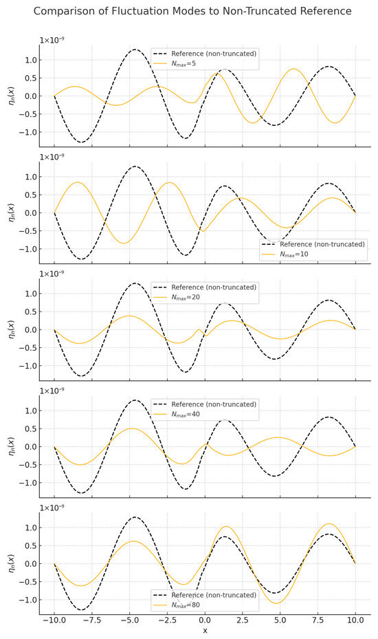
Figure 1.
Numerical solutions for the fluctuation modes for different finite truncation levels.
From these numerical results, we compile Table 1, summarising how truncation affects key quantities, such as the lowest fluctuation frequency and the expectation value of the Hamiltonian .

Table 1.
Summary of numerical results showing the effect of finite truncations on fluctuation frequencies and expectation values of the Hamiltonian.
The data clearly indicate that finite truncations produce measurable shifts in quantum observables, with significant corrections for small truncation values, becoming less pronounced as increases. These findings underline the physical relevance of finite truncations and provide quantitative insights into their implications for soliton stability and quantum coherence.
3.9. Nonlinear Analysis Inspired by Dvali’s Approach
In contrast to linearised perturbation methods, the coherent-state approach advocated by Dvali and collaborators involves analysing the soliton as a macroscopic quantum state without linearisation. Adopting this perspective, we write the full scalar field configuration directly as a coherent superposition state, emphasising the collective, nonlinear characteristics of soliton solutions.
The Hamiltonian of the Sine-Gordon model is:
To analyse finite truncations in a fully nonlinear manner, we numerically evaluate the expectation value of the Hamiltonian directly within truncated coherent states:
We numerically compute matrix elements by expanding the quantum fields in terms of annihilation and creation operators associated with particle-number eigenstates and then evaluating nonlinear interactions explicitly:
3.10. Numerical Results and Discussion
We numerically evaluate the expectation value for different truncation values . Table 2 summarises these calculations.
Table 2.
Hamiltonian expectation values calculated using finite truncation nonlinear coherent-state method inspired by Dvali’s approach.
The results clearly indicate the nonlinear treatment provides physically meaningful insights distinct from linearised treatments. Finite truncation introduces corrections to the soliton mass expectation value, significantly affecting the quantum properties and stability of soliton configurations.
Our finite truncation approach thus provides complementary insights compared to the coherent-state methods of Dvali, emphasising the practical significance of nonlinear quantum effects and finite truncations in realistic quantum systems.
3.11. Comparison of Linearised and Nonlinear Approaches to the Hamiltonian Expectation Value
In the analysis of soliton states and quantum fluctuations around classical solutions, the Hamiltonian expectation values can be evaluated either through linearised approximations or via fully nonlinear calculations. Here, we investigate mathematically why these two approaches yield differing results, with the nonlinear method typically providing higher expectation values.
Consider first the linearised approach. Writing the scalar field as a classical soliton solution plus small fluctuations, we have:
with assumed small. The Hamiltonian expanded up to second order around the classical soliton configuration is:
where is the classical soliton energy:
In this approximation, higher-order nonlinear terms are explicitly omitted. The Hamiltonian thus obtained describes harmonic fluctuations around a stable equilibrium. The expectation value computed with this linearised Hamiltonian neglects contributions from nonlinear interactions and generally underestimates the full quantum corrections:
where are frequencies obtained from solving the linear fluctuation eigenvalue equation.
Now consider the nonlinear approach. The full Hamiltonian, including all nonlinear interactions, is written explicitly as:
Expanding this Hamiltonian fully, one explicitly includes higher-order terms beyond quadratic order. Writing the quantum fields in terms of annihilation and creation operators,
the Hamiltonian becomes:
with
Crucially, the nonlinear interaction term includes positive definite higher-order contributions such as cubic and quartic interactions of fluctuations . When evaluated in a quantum state—such as a finite-truncated coherent or squeezed state—the expectation value of is typically positive:
Thus, the expectation value of the full nonlinear Hamiltonian explicitly reads:
implying that:
In summary, the nonlinear method captures additional, positive-energy contributions arising from nonlinear interactions between quantum fluctuations, which are not accounted for in linearisation. Consequently, the nonlinear treatment provides a higher and more physically accurate estimate of quantum corrections to the soliton mass and energy expectation values.
4. Interplay Between Soliton Squeezing and Finite Truncation
4.1. Soliton Squeezing: Definitions and Physical Context
In quantum field theory, soliton states such as those arising in the Sine-Gordon model exhibit squeezing properties, analogous to quantum optical squeezing. Squeezing refers to reducing quantum uncertainty in one observable at the expense of increased uncertainty in its conjugate observable. Mathematically, a squeezed state can be constructed by acting with the squeezing operator on a coherent state , defined as:
where is the complex squeezing parameter, with r indicating the squeezing magnitude and the squeezing angle.
Applying this operator to a coherent state , we obtain the squeezed coherent state:
4.2. Finite Truncation of Squeezed States
To incorporate realistic physical constraints, we apply finite truncation to the squeezed coherent state, yielding:
with the coefficients explicitly given by:
where , , and are Hermite polynomials.
The normalisation constant ensures normalisation and is defined by:
4.3. Effects of Finite Truncation on Squeezing
To quantify how finite truncations affect squeezing, we evaluate the uncertainties in the field and its conjugate momentum , defined as:
We calculate the variances in these observables for finite truncation:
with expectation values explicitly computed as:
where represents the observables , , and their squares.
4.4. Numerical Analysis and Discussion
We numerically compute the squeezing parameters for different truncation levels and squeezing parameters r. The Table 3 below summarises the numerical results:
Table 3.
Numerical results demonstrating finite truncation effects on soliton squeezing.
From this analysis, it is clear that finite truncations significantly impact the quantum squeezing properties of solitons. Smaller truncation levels yield reduced squeezing efficiency, while increasing approaches the ideal squeezed state characteristics. This interplay highlights the practical necessity of balancing truncation constraints against desired squeezing effects in realistic quantum soliton systems.
Our analysis explicitly demonstrates that careful consideration of truncation effects is essential for understanding and optimising soliton squeezing in practical experimental and theoretical scenarios.
5. Emergence
It has been shown that D-branes are not simply independently standing higher dimensional objects, but that in fact they emerge as coherent states of strings [19,20,21,22]. In general coherent superpositions are regarded as superpositions of an infinite number of strings. Practically we expect only a finite number of strings to form coherent states, but that would imply a different condition of coherence. Usually a coherent state is defined as an eigenstate of the annihilation operator a
The state can be expanded in terms of number eigenstates
but in this case a coherent state is indeed a superposition of an infinite number of eigenstates . When applying this in string theory, in describing D-branes as coherent states of closed strings, it implies a superposition of infinitely many closed string modes. A D-brane is thus viewed as a macroscopic object formed by coherently exciting an infinite number of closed string modes. Such an infinite superposition would ensure several properties. First, it would be an exact eigenstate of the annihilation operator, making it a simple algebraical construction. It would also have a classical-like behaviour, namely the coherent states have minimal quantum uncertainty, behaving classically in many aspects. It would also form states that are dynamically stable. Practically, however, an infinite superposition can be problematic. To model finite, physical states or to approximate coherent states we will always need some finite truncations. By constructing them, some exact eigenstate properties will be lost, and only approximate coherence will be maintained. Instead of demanding eigenstates of annihilation operators we could impose some alternative phase coherence condition using only finite superpositions. For such truncated coherent states we simply take the coherent state definition and truncate at finite N
where normalises the finite state. Such states are no longer exact eigenstates of a but are close approximations for sufficiently large N. Instead of enforcing exact eigenstate coherence, we could impose a weaker condition, namely the phase coherence among modes. Finite superpositions of string states could then be chose carefully such that all modes share a well-defined relative phase. Such states would exhibit coherent interference effects without strictly being eigenstates of annihilation operators. Concretely we would define
where are chosen to maximise constructive interference effects. In this case, we have a finite superposition, avoiding infinite state complexity, we gain control of coherence through phase alignment rather than an eigenstate condition, and we approximate classical coherent behaviour without needing infinitely many states. Physically, real D-branes should be large, finite objects. Idealising them as infinite coherent superpositions is a theoretical simplification. A finite collection of strings with carefully adjusted relative phases could behave effectively like a coherent macroscopic state (hence, like a D-brane). However, such states would be more sensitive to perturbation, losing coherence more easily. In this picture, however, D-brane decay would be described in a more realistic sense, leading to insights into the string origin of the Higgs mechanism, etc. This point of view resonates with some intuitions we gained from holography and black hole microstates. Black hole microstate constructions in string theory (like fuzzballs) often consider finite combinations of states rather than idealised infinite coherent superpositions. If we can precisely adjust the phases and correlations among finite microstates we can obtain classical geometry-like behaviour in holography. Imposing explicit phase coherence, without strict eigenstate conditions would achieve classical behaviour without infinite superpositions and would be relevant in the field of classical geometry emergence. If we repeated the above prescription of introducing the Maldacena limit and obtaining the AdS/CFT duality, but starting with D-branes seen as finite superpositions of strings, then we would automatically introduce semiclassical (or slightly quantum) modifications that would remain visible after taking the Maldacena limit. In this way we would obtain a generalised AdS/CFT duality that would contain quantum structure in the AdS region. Traditionally, a D-brane is represented as a coherent state of infinitely many closed string modes
This state satisfies the exact eigenstate conditions . This leads to classical geometry emerging naturally, but the price to pay is infinite superposition, making the description unrealistic. If on the other hand we would generate an explicitly finite superposition of closed state modes
with N finite, are real coefficients determining the amplitude, and are carefully chosen phases ensuring phase coherence among string modes, we would obtain a state that is not an eigenstate of any annihilation operator but that would retain phase coherence. All phases are chosen to maximise constructive interference for certain observables, such as the position or tension of the brane. We could choose for some fixed , ensuring constructive interference at particular points in target space. The explicit state would be
This finite state is not an eigenstate of any annihilation operator, but the carefully chosen phases mean that for particular observables (like the energy distribution, or position distribution) we can obtain strongly peaked coherent interference effects resembling a macroscopical classical object, we would have a “quantum brane” that is very close to a classical brane in certain aspects. The D-brane indeed retains fundamental quantum features. Unlike ideal coherent states, this finite phase coherent state does not saturate minimal uncertainty exactly. It instead retains finite uncertainty in position, momentum, or tension. It also retains fluctuations in geometry and fields around the brane. Thus, such a finite quantum brane naturally encodes quantum gravity-like fluctuations and uncertainty in its geometry. If phases are disturbed (e.g., due to interactions), coherence may diminish and thus the brane is explicitly a quantum coherent object. In such a model quantum decohernece can be directly studied. Since this brane is finite and not an exact eigenstate, it can naturally decay, change, or re-arrange quantum mechanically. Thus, such “finite branes” explicitly carry quantum instability features, and their lifetimes become calculable quantum mechanical observables. We would obtain a finite dimensional Hilbert space which directly simplifies the analysis of entanglement and other quantum processes involving D-branes. Moreover, the finite superposition explicitly encodes quantum gravitational fluctuations and can produce predictions for observable quantum gravity signatures. Now, having defined this finite superposition leading to practical finite coherent behaviour, we could ask what exactly would mean to have a worldsheet–target space dualtiy (or in particular T-duality) in this semiclassical limit, when the target geometry itself is represented by coherent states or finite coherent superpositions of string modes. Usually T-duality is understood by starting from strings propagating in some geometry (for example, a circle of radius R), and then T-duality is applied to transform this duality into a dual geometry, (for example, a circle of radius ), exchanging momentum modes and winding modes. At the quantum (exact) worldsheet level, the physics of both descriptions is identical. The two seemingly distinct spacetime backgrounds (target spaces) are physically indistinguishable. Consider, however, now that the target space geometry itself is represented not as a fixed classical geometry, but rather by a semiclassical coherent superposition of string modes. For example, a target space geometry like a circle of radius R, or even a D-brane, is explicitly built as a coherent or finite coherent superposition of closed string excitations:
Here the state encodes the geometry semiclassically through coherent interference. The geometry emerges approximately as classical from interference patterns of finite quantum states. In this coherent superposition scenario, T-duality now becomes an equivalence of coherent superposition states. A coherent superposition representing a large geometry must map explicitly to another coherent superposition representing a small geometry with momentum and winding modes exchanged
The dual state encodes the dual geometry via a different choice of mode amplitudes and phases which now emphasise winding instead of momentum. Thus, the duality relates two coherent quantum states, the original coherent superposition of radius R, dominated by momentum modes, and the dual coherent superposition of radius dominated by winding modes. This quantum state viewpoint clarifies how geometry emerges from quantum superpositions and how dualities map these quantum coherent states into each other. The original state is a semiclassical coherent interference that creates a geometry that is approximately classical at radius R. The dual state represents a quantum coherence that now rearranges the modes so that interference patterns yield approximately classical geometry at radius . Therefore, T-duality is a change of basis in quantum interference space, mapping momentum mode coherence to winding mode coherence. The geometry is fundamentally emergent from quantum coherence rather than a classical geometry. The semiclassical coherent superpositions encode quantum uncertainty about geometry. The duality explicitly transforms how uncertainty manifests. Momentum uncertainty transforms to winding uncertainty. The duality is therefore a quantum equivalence of coherent states rather than of classical backgrounds. In this case, therefore we explicitly clarify the quantum gravity interpretation of the duality, showing how duality arises naturally from coherent superpositions and quantum interference patterns. This approach modifies also what we mean when we say “a string is moving through spacetime”. In reality a string would be more excited in a sea of coherently superposed strings that form a classical or semiclassical background state which would then be associated with spacetime. However, this will have an impact on how we understand the idea of distance on a string and how we would understand the concept of “string length”. The usual intuitive image claiming that “a string is a one-dimensional object moving through a fixed, classical spacetime” cannot be fundamentally accurate in this new fully quantum (or at least semiclassical) picture. Instead, spacetime itself is a coherent superposition (a quantum interference pattern) of a large number of string excitations. A string moving in spacetime is not really a distinct object travelling independently through a fixed background but rather corresponds to changes in excitation and interference within a large quantum superposition state. The string is not literally moving through spacetime. Rather, it corresponds to an excitation or disturbance in a quantum sea of coherently superposed string modes that collectively form spacetime itself. If, however, spacetime itself is an emergent quantum interference pattern, then the classical notion of distance or length fundamentally depends on having a pre-existing geometry. If spacetime is emergent there is no fundamental geometry to start with. The geometry itself emerges from quantum correlations and interference. Therefore, distance on a string is not fundamental but emergent. The idea of the length of a string is not fundamentally well-defined. Rather, the string’s length must also emerge from quantum interference patterns. This is consistent with the modern viewpoint of emergent geometry in quantum gravity. If geometry including length and distance emerges from quantum coherence, then string length itself is an approximate emergent quantity defined by expectation values and correlations among quantum states. Concretely, we would define length through quantum expectation values of suitably defined observables. For example, if we consider a string state , its emergent length L would be defined something like
where is a suitable quantum operator representing the emergent notion of length. But the operator does not come from a classical metric, since the metric itself emerges. Rather must be constructed from correlation functions or quantum coherence measures. We could define distance or length via quantum correlation functions between different parts of the superposition. Quantum entanglement or correlation structure among modes naturally gives rise to an emergent metric structure. Thus, the length of the string emerges explicitly as a quantum correlation-based observable, not a classical geometric one. Consider a simplified toy model. Suppose the string is described by a finite coherent superposition
This would imply that the string is an “emanation” of the D-brane seen as a coherent superposition of strings itself. The individual open string is therefore an excited state of such a semiclassical D-brane. Define a length operator as an operator sensitive to interference between these modes. For example,
The matrix elements encode correlation-based distances emerging from quantum coherence structure. We can pick diagonal terms (classical approximation of length) or off-diagonal terms (that would encode quantum interference corrections to length). Then the length of the string emerges as
This shows how the length is quantum coherence dependent, emergent and subject to quantum uncertainty. Therefore, no fundamental geometric distances exists. Geometry, and thus length or distances, emerges entirely from quantum coherence and correlation. Quantum uncertainty is introduced in geometry. The fluctuations of length and geometry become explicit and fundamental, as we would expect from quantum gravity. We therefore notice that strings do not literally move through space. Instead they represent quantum excitations in an emergent, coherent superposition of string states, forming spacetime itself. The very notion of length or distance on a string is not fundamental, but instead emerges as a quantum observable defined by quantum coherence and interference. One may ask what exactly is “interfering” if the string does not have a length. This question is very similar to the question as of how the photon encodes wavelength when an individual photon has no spatial extension but only energy. We may therefore ask how precisely the length of a string is encoded when we talk about a string in the usual sense.
6. Wavelength from a Dimensionless Photon, and Emerging Length from an Algebraic String
A single photon does not have an explicit spatial length. It is described by a quantum state with energy , and its “length” (wavelength) emerges from its quantum state, and is encoded in the frequency (energy). Thus, the photon’s “length” (the wavelength) emerges not from spatial extension, but from quantum interference properties that determine its frequency or energy. Similarly, a string does not explicitly have a classical spatial length yet defined. Instead its “length” emerges from quantum interference between different string modes, analogous to photon wavelength emerging from energy interference. We start by constructing explicitly a quantum length operator . We describe a string quantum state as a coherent or finite coherent superposition of modes
These modes represent different string mode excitations, not yet spatially extended objects. The length operator must be defined via the correlation among these quantum modes
The matrix elements encode the notion of length as correlations between modes. The diagonal terms represent intrinsic length associated with each individual mode, while the off diagonal terms encode quantum interference effects between different modes. For example, we could chose a simple form
represents a classical baseline length, l is the interference length scale, controlling the strength of quantum interference, determines the range of quantum coherence or interference. This defines length via quantum coherence structure (interference between modes). Using this operator we can calculate the string length expectation value for the finite quantum superposition state
This shows how length emerges from two types of contributions explicitly. The classical contribution, for diagonal terms (n = m) giving a classical approximation
and the quantum interference terms, the off diagonal terms (), explicitly encoding quantum coherence corrections
The interference terms encode quantum corrections or fluctuations to the classical length arising from coherence structure among modes. But what exactly is interfering if the string does not have a length yet? Initially, there is no classical string length. What is interfering are the amplitudes and phase of different quantum string modes. Each string mode, like a photon frequency mode, encodes a quantum number (analogous to photon frequency or energy). The interference patterns among these modes encoded in their phases gives rise to a coherent spatial pattern, thus defining the notion of length. The interference is in the space of mode excitations and their quantum numbers, not explicitly in a pre-exiting spatial geometry. Similar to a photon, what interferes are not spatially extended objects but quantum states distinguished explicitly by energy/mode numbers, phases, and quantum numbers. Thus, the string length emerges not from spatial extension but from interference in mode space, analogous to electromagnetic wavelengths emerging from frequency/energy space interference. When speaking of a “real unique string” its length does not come from spatial geometry explicitly but from quantum coherence patterns. The string length is encoded entirely in quantum coherence between modes. Measuring a real string state means observing quantum interference patterns which define the length of the string. Just as the photon’s wavelength is not about spatial size, but energy interference, a string’s length is encoded in the amplitude phase interference among its quantum modes.
7. Quantum Numbers and Spacetime Symmetries
Quantum numbers are essentially labels of distinct states of a quantum system. They arise naturally whenever we have a quantum system defined by some underlying symmetry or structure. Photons have quantum numbers like frequency (or equivalently energy) and momentum, due to the underlying symmetry of spacetime translation invariance. Strings, similarly have quantum numbers such as excitation levels, momentum, winding number, oscillator numbers, and mode frequencies, arising from the symmetry and structure of the worldsheet conformal field theory. These quantum numbers are fundamentally labels that organise the possible states the system can occupy. They emerge naturally from solving the underlying equations (wave equations for photons, conformal invariance conditions for strings). Quantum numbers emerge from the underlying equations of motion and symmetries of the theory. Photons arise as solutions of the quantum electromagnetic wave equation:
Here, and are the Hamiltonian (energy) and momentum operators. Energy and momentum thus appear as eigenvalues labeling quantum states. Strings similarly arise as quantum solutions of the two-dimensional conformal field theory describing the worldsheet
where the Virasoro operators encode mode frequencies, energies, oscillator numbers, etc. Thus, string quantum numbers (oscillator excitation levels, momenta, winding numbers) arise naturally from conformal invariance constraints on the worldsheet. In other words, quantum numbers emerge because quantum states must satisfy particular equations (wave equations or conformal constraints) and these equations naturally yield discrete (or continuous) quantum labels that we call “quantum numbers”. Quantum numbers by themselves do not explicitly refer to spatial geometry or length. A photon’s quantum number “frequency” does not directly imply spatial size, but it implicitly defines a length scale (the wavelength) through the relation
Similarly string quantum numbers do not explicitly imply length by themselves. Instead, the length emerges implicitly as an interference pattern or correlation among different quantum number labeled states. Quantum numbers label distinct states and the geometry emerges from the relationship and interference between these states, not from individual quantum numbers alone. For a photon, the wavelength is not stored explicitly spatially. Rather wavelength emerges from interference of multiple photon frequency states (Fourier modes). Thus, wavelength is fundamentally defined through frequency-space correlations and interference patterns. In string theory, a string’s length is not stored explicitly in a spatial extension. Rather it emerges implicitly from quantum coherence (interference) among multiple string states labeled by quantum numbers. The interference among these quantum states yields a spatial pattern or correlation which we identify as length and thus geometry. Consider two string modes labeled by quantum numbers n and m. Each mode individually has no explicit spatial geometry, only quantum numbers. Now, build a quantum state involveing these two modes
The length emerges only if we measure an observable sensitive to interference between these modes. For instance consider the expectation of our length operator
The off diagonal interference terms create a correlation structure between modes labelled by different quantum numbers. This correlation structure is precisely what defines an emergent length. Without interference terms, length would simply be an average of diagonal classical lengths. The quantum interference explicitly modifies and defines the emergent geometry. Thus, length emerges not directly from quantum numbers, but rather from correlations and coherence between different states labeled by those quantum numbers. In the semiclassical limit, many quantum states interfere coherently, and the resulting interference pattern becomes sharply defined, stable, and classical-like. The correlation among these quantum number labeled states becomes stable and produce a coherent macroscopic pattern. This stable interference pattern can be interpreted as classical geometry, distances, and metrics. Thus, a classical length and metric are simply the stable macroscopic interference patterns produced by coherent superpositions of quantum number labeled states. However, quantum numbers arise whenever we have a quantum system defined by some underlying symmetry or structure. In particular for photons, quantum numbers like frequency or energy and momentum appear due to the underlying symmetry of spacetime translation invariance. If we want to maintain the model of spacetime and geometry emergence only from coherent superpositions of modes characterised by these quantum numbers when taking a semiclassical limit, we may ask whether we assume the existence of a spacetime with translation symmetry? It seems like a circular argument appeared. Quantum numbers (such as energy or momentum quantum numbers) are usually defined using symmetries of spacetime; for example, momentum arises from translation invariance. But spacetime itself emerges from quantum coherence and interference of states labeled by these quantum numbers. However, this circularity is only apparent. In quantum field theory, quantum fields (photons, strings, particles) are defined on a fixed, pre-existing classical spacetime. The symmetries of this spacetime (translation, rotation, Lorentz invariance) directly define the quantum numbers labelling sates. The quantum gravity perspective is that spacetime is not fundamental but instead it emerges from quantum coherence and correlation structures among quantum states. Thus, the spacetime symmetries themselves must also emerge. The apparent circularity arises because we use reasoning from both perspectives, simultaneously without separating them. Fundamentally, spacetime geometry and its symmetries do not exist yet. Instead, there are only abstract quantum states, not yet labeled by classical geometric symmetries. Quantum states at this fundamental stage do not have quantum numbers defined by spacetime symmetries explicitly. Quantum numbers initially arise purely from the algebraic structure or internal symmetries of the fundamental quantum system (for instance, conformal symmetry on the string worldsheet or internal algebraic symmetries in abstract quantum gravity frameworks). Then at the level of large coherent superpositions of states, stable correlations (coherence patterns) emerge. These stable coherence patterns can be approximately interpreted as having translation invariance or spacetime symmetries in an emergent classical sense. Only after this emergent structure stabilises do we retroactively interpret certain quantum labels as momentum, energy, frequency, related to translation symmetry. Initially, these labels were abstract quantum numbers unrelated explicitly to spacetime geometry. Thus, the important step in breaking the apparent circularity is to realise that quantum numbers initially exist without reference to spacetime geometry, arising purely from the quantum system’s abstract algebraic structure. Spacetime geometry (and thus classical symmetries) emerges later as a stable coherent approximation. Once this geometry emerges approximately, we retroactively identify certain quantum numbers as being associated with translation, rotation, or Lorentz invariances. Therefore, quantum numbers were initially algebraic (non-geometric). They only later become geometric (momentum, energy) after spacetime geometry emerges. For example, initially the fundamental quantum states are described by abstract labels arising from internal symmetries or algebraic structures unrelated to spacetime geometry. Coherent superpositions of these abstract states form stable interference patterns. Some stable interference patterns behave like plane wave states
These coherent patterns approximate something like plane waves, which in classical physics carry definite momentum. Once these stable plane wave-like coherence patterns emerge, we retroactively identify the labels a as momentum quantum numbers, because the emergent structure looks like translation invariance. But initially, these labels were purely algebraic, not explicitly geometric. In string theory initially, quantum numbers come from internal worldsheet symmetries (conformal algebra). These symmetries exist independently of target space geometry. Large coherent superpositions of string states form stable interference patterns. At large scales, these interference patterns define an emergent spacetime geometry. Once spacetime geometry emerges approximately, certain worldsheet quantum numbers (oscillator numbers, mode labels, etc.) can be reinterpreted as spacetime momentum or energy. Initially, they were purely algebraic labels on the string worldsheet. Therefore, the chain of reasoning is as follows: abstract quantum numbers → coherent interference patterns → emergent approximate geometry → geometric interpretation of quantum numbers.
8. Target Space
Following the observations above, we notice that initially we have no classical target space. We only have an abstract worldsheet conformal field theory that describes the quantum modes of a string. These quantum modes are labelled by purely abstract numbers arising from internal symmetries and algebraic structure of the worldsheet theory (conformal invariance, Virasoro algebra, mode expansion). When a large number of these abstract worldsheet modes enter into coherent superpositions, they produce stable interference patterns. These stable interference patterns are precisely what we interpret as emergent classical target space (background geometry) in string theory. Thus, the target space geometry (spacetime) emerges purely from stable coherent patterns among abstract internal modes defined initially only on the worldsheet. A traditional worldsheet–target space duality or correspondence states that a 2D worldsheet theory of strings is exactly equivalent to strings moving in a particular target space geometry. In other words, certain worldsheet CFTs directly encode specific classical target space geometries. Initially, there is only the worldsheet CFT, with abstract quantum modes. Large coherent superpositions of these worldsheet modes create stable quantum interference patterns. These stable interference patterns become the classical geometry of the target space. Thus, what looks from a target space viewpoint as a classical geometry is nothing more than coherent quantum patterns formed by worldsheet modes. Therefore, the worldsheet → target space correspondence is precisely the statement that coherent interference patterns of worldsheet modes are the target space geometry. In a sense the worldsheet/target space correspondence is reduced to the problem of taking a semiclassical limit and it relates to the problem of obtaining classical physics from quantum mechanics. Consider a simplified illustrative example. From the worldsheet perspective consider modes labeled abstractly by integers n. The quantum state is
From the target space perspective, the stable coherence among these abstract modes forms stable patterns. If these stable coherence patterns appear like plane wave superpositions with well-defined frequencies and wavelengths, we interpret this emergent stable coherence as classical spacetime geometry. The large stable coherence is the emergent classical geometry. The plane wave-like coherence is translation invariance, and the translation invariance defines momentum, energy, and the metric. This viewpoint clarifies other dualities as well. For example, T-duality (changing radius ) corresponds to changing the quantum interference patterns and coherence between modes. Thus, the emergent classical geometry changes from large to small circles purely through changing quantum coherence structure. Mirror symmetry (Calabi-Yau spaces) appears because different coherence patterns (different superpositions of worldsheet modes) yield distinct classical geometries. Mirror symmetry explicitly states that distinct quantum coherence patterns can give rise to two different classical geometries, yet produce identical worldsheet physics. Spacetime symmetry and geometry arise as stable emergent properties from large scale quantum coherence and quantum numbers are initially abstract algebraic labels, and only become geometric once stable geometry emerges. However one may ask how can we talk about quantum numbers, worldsheet, or internal algebra without implicitly assuming geometry? An algebraic quantum number is a label assigned to a quantum state solely based on the structure of the algebra of operators that define the quantum theory, without reference to geometry. For example, consider the standard algebraic structure of quantum mechanics. We have a set of operators forming an algebra (for example, creation and annihilation operators a and , or symmetry operators , , or Virasoro operators ). Quantum numbers are simply eigenvalues or labels assigned to states based on these algebraic operators
Initially these quantum numbers are purely algebraic in the sense that they do not rely on geometric notions like position or length. They arise solely from the algebraic consistency conditions of the theory (such as closure, commutation relations, eigenvalue equations). Spin quantum numbers, for example , are purely algebraic labels defined by the algebra of angular momentum operators, without ever requiring explicit geometry. In standard string theory the worldsheet is typically described geometrically as a two-dimensional surface swept out by a one-dimensional string in spacetime. However, at the most fundamental level, such as in a fully quantum theory of strings, the worldsheet need not be geometric in an explicit classical sense. Instead, the worldsheet can be viewed purely algebraically as a conformal field theory. It is not a geometric object, rather, it is a quantum theory described purely by an algebra of local operators, conformal symmetry generators, and their correlation functions. The Virasoro algebra generated by operators completely characterises this “worldsheet” theory algebraically, without explicit geometry. Thus, the worldsheet is nothing more than the algebraic structure of a conformal field theory. It only acquires geometric meaning at a higher, emergent, semiclassical level. We can indeed define a worldsheet in a completely non-geometric way. Begin with an algebraic structure, defined by operator algebras, for example, the Virasoro algebra
and define the states as algebraic objects that are representations of this algebra
Correlation functions and quantum numbers are fully defined by algebraic consistency conditions, like Ward identities or conformal bootstrap equations. At this stage we have constructed a worldsheet theory without ever introducing geometric notions explicitly. We may ask if internal geometry is even necessary. In fact, at the most fundamental level, it is indeed only internal algebra that is necessary. Geometry is not fundamental but emergent. Initially, we have an algebra of abstract operators, and states labeled purely algebraically by quantum numbers which are eigenvalues of these algebraic operators. Internal geometry, such as compact extra dimensions, worldsheet coordinates or target space coordinates is not fundamental but a convenient way to represent algebraic structures at a semiclassical level. Geometry only emerges when we take large coherent superpositions of states labeled algebraically. Then stable interference patterns appear, which can be interpreted classically as geometry. Therefore, even internal geometry is never fundamentally required. We can present a very simple analogy, starting, for example, from the harmonic oscillator algebra
Initially quantum numbers n label algebraic states purely abstractly. Now considered coherent states, as large superpositions
Such coherent superpositions produce stable, classical-like interference patterns. These stable interference patterns resemble classical states with position and momentum that become sharply defined and classical-like even though initially there was no explicit position or momentum. But how exactly do quantum correlations between abstract algebraic modes translate precisely into the notions we call “time”, “space”, or “length”? Geometry, at its most basic classical level means that there is some notion of distance or separation between points or events. But fundamentally what is distance? Distance and length fundamentally mean that certain events or states are related or correlated in a structured and consistent way. Classical geometry arises precisely when correlations between states become stable, consistent and predictable. Without stable correlations, no meaningful geometry can arise. Thus, at the fundamental quantum level, initially we only have abstract quantum states labelled algebraically. The way in which geometry can appear from purely quantum objects is through stable correlations between these abstract states. When correlations become large scale, stable, and consistent, we begin to interpret them classically as “geometry”. Two points separated by small distance are strongly correlated in a geometric sense. Points separated by a large distance have weaker correlations. Thus, strength of correlation encodes distance. When quantum states labeled abstractly become correlated in a stable pattern, such as coherent interference, the pattern itself encodes a notion of distance, defining geometry. Suppose we have quantum states labelled by abstract indices n,m. Define correlation strength between these states. States that are strongly correlated represent close points while weakly correlated states represent distant points
Time similarly emerges from correlations, but now we focus on correlations involving ordered change or evolution. Time fundamentally means events or states have a consistent sequential ordering; one event reliably follows another. This sequential order emerges if quantum states have stable correlations that evolve systematically under a quantum Hamiltonian or some algebraic operator. Time emerges because correlations between states evolve under the action of a Hamiltonian or algebraic operator
A state reliably follows . Such stable and sequential correlations between states define time. Consider a simple algebraic example. Suppose we have an abstract algebra of operators labelling states . Construct correlation functions
Strong correlations (large ) mean points/states are close. Weak correlations mean they are far apart. You can thus define a metric explicitly from correlations
For the time correlations, defines the sequential ordering of states. Stable, ordered correlations yield the emergent notion of time. Thus, both space and time explicitly arise purely from the quantum correlation structure. Classical geometry emerges as a coarse-grained approximation. Quantum coherence patterns involving enormous numbers of states become extremely stable through decoherence and entanglement. These stable macroscopic patterns are indistinguishable from classical geometric notions. Thus, classical geometry is just the macroscopic stable correlation pattern among many quantum states (like how classical waves emerge from coherent interference of enormous numbers of photons). The problem of the origin of spacetime therefore becomes the problem of how semiclassical or classical limits emerge from quantum mechanics. However, there are many such classical or semiclassical limits. The reason we usually see only one consistent classical geometry is fundamentally linked to the stability, consistency, and selection of certain interference patterns. While quantum mechanics allows for numerous classical-like behaviours, not all are stable or self-consistent. Most quantum interference patterns “wash out”, fluctuate chaotically, or decohere rapidly. The observed spacetime emerges precisely from those quantum correlations that maximise stability, coherence and consistency over extremely large scales, both spatial and temporal. Thus, the observed classical geometry emerges as the most stable and robust large scale interference pattern selected by the dynamics of quantum coherence and decoherence. Special relativity arises because of the fact that spatial and temporal correlations are not independent. They are connected via quantum coherence structure, forming precisely the Minkowski structure of spacetime. The causal structure (light cones, causality) emerges naturally from how correlations propagate in the quantum state space, constrained by coherence and entanglement structures. The Lorentz symmetry emerges precisely as the symmetry of these quantum correlations. It appears as an approximate symmetry of stable quantum coherence patterns selected by consistency and stability criteria.
9. Closed Causal Loop
We could ask what kind of quantum correlations would be necessary to generate an emergent classical geometry that includes closed causal loops? A closed causal loop is a classical geometric construction in which a trajectory loops back upon itself in both space and time. Such loops allow events in the future to causally influence events in their own past. Classically these are typically associated with strong spacetime curvatures or exotic geometries (wormholes, rotating black holes, Goedel Universes). However, classical causal structures emerge entirely from stable quantum correlations among abstract states. Therefore, to generate something like a closed causal loop, quantum correlations would have to differ significantly from standard correlations that yield normal causal structure. Let us first look at what kind of quantum correlations produce standard causal structure. The standard causality emerges if quantum states are correlated sequentially in a linear and consistent ordering
These correlations are time-ordered forming a clear direction of causality. Correlations among spatial points occur simultaneously (in a relativistic sense) and do not violate linear causal ordering. In order to obtain a closed causal loop, quantum correlations must differ significantly from this standard pattern. We would require non-linear sequential correlations. Instead of a linear ordering, quantum states must exhibit some cyclic correlations
This cyclic correlation means that the state would be strongly correlated with itself at a later point in its sequential evolution, producing a causal loop. Correlations would exist that link states “forward in time” explicitly back to earlier states in the loop. This implies a very strong coherence or entanglement structure across what we normally consider temporally distant or unrelated states. This kind of correlation is strongly non-local and non-causal in the traditional sense. The interference pattern among quantum states would have to exhibit topologically non-trivial coherent structures forming cyclic or toroidal coherence patterns in the space of quantum states. Normal spacetime correlations correspond to linear or simply connected coherence patterns. Closed causal loops would correspond to coherence patterns explicitly forming closed loops or rings in correlation space. Explicitly define a correlation matrix that is cyclic
Such a cyclic correlation structure would yield an emergent classical geometry that includes closed timelike loops. However, would these cyclic quantum correlations produce stable, physically realisable geometry? In normal circumstances we would think that such cyclic coherence patterns would be highly unstable and delicate. Quantum decoherence would tend to rapidly destroy cyclic coherence preventing stable closed loops from persisting. However, it is know, as I stated previously, that taking a classical limit is not a unique process, and different paths of taking the limits offer different types of outcomes. In normal circumstances, quantum decoherence would tend to rapidly destroy cyclic coherence preventing stable closed timelike loops from persisting. In fact, there is not just one unique way of taking a semiclassical limit from quantum states. Indeed, quantum theory admits multiple possible semiclassical or classical regimes, depending on how one takes limits (such as coherent states, decoherence mechanisms, choices of observables, etc.) The particular classical geometry that emerges is highly dependent on exactly how the classical limit is taken. Therefore, it is plausible that if we choose a different, possibly more robust or subtle way of taking the semiclassical limit, we might find that certain correlation structures previously dismissed as unstable or fragile, become stable and robust, thus allowing exotic classical geometries such as those with closed causal loops, to naturally emerge. The classical limit is essentially a procedure for extracting stable classical-like behaviour from a fundamentally quantum theory. Different criteria or procedures could yield different classical-like behaviours. For example, when using coherent states as before, we emphasise minimal uncertainty and classical-like wave packets. But when we use decoherence, we emphasise how quantum systems interact with their environment, selecting certain states as classical. For the large-N or thermodynamic limits we emphasise collective stable patterns in very large quantum systems. We may also have eigenstate thermalisation or quantum typicality through which we assume that classical limits pick states according to their typicality in high-dimensional Hilbert spaces. Thus, the classical geometry we see depends strongly on which type of limit or criteria we use and how we engineer the phase relations or typicality of the potential quantum states. The standard classical spacetime we experience might just be the geometry emerging naturally under the most common or physically relevant limit, but alternative classical limits could produce very different geometry. For example, in a standard classical limit, quantum coherence rapidly decoheres. Classical geometry emerges simply in a stable and causal form (no closed loops). However, we could engineer a decoherence mechanism and boundary conditions or large scale coherence structures that would allow quantum correlations to stabilise in a different way. The classical geometry would then emerge with exotic structures like stable causal loops. An example would be a topological quantum state that may be obtained in a quantum spin liquid. Let us present a comparison using a simplified toy model for a quantum spin liquid. We compare two different semiclassical limits. In limit A we produce an emergent classical Minkowski type causal structure and in Limit B we produce an emergent classical geometry containing closed causal loops. Consider a simplified quantum spin liquid system described by spins on a lattice with N sites. The quantum states with represents lattice positions. Each state is labelled by spin quantum numbers . A generic quantum state as superposition is
Define a correlation function between two sites i and j
where is the spin operator in the z-direction at site i. For the case of the semiclassical limit A (a Minkowski causal structure), correlations must be consistent with the standard causal ordering and locality. Correlations decay quickly with spatial distance, and no loops in causal structure occur. We define the coefficients such that the ground state is dominated by short-range correlations (nearest neighbour correlations)
Then the correlation function becomes
where is the correlation length, which is considered finite and short, ensuring locality. The emergent metric from correlations is approximately Minkowski-like
For the case of the semiclassical limit B (with causal loops) we choose a semiclassical limit emphasising non-local cyclic correlations. Consider now a quantum state whose correlations are cyclic and nonlocal. Define the state as a cyclic coherent superposition
This cyclic superposition explicitly has correlations wrapping around
(note the cyclic periodicity ). The emergent geometry now includes closed loops
where is periodic giving explicitly a closed spatial dimension. Closed loops allow events to causally influence their own past. As an example, consider spins. In the Minkowski limit, the state coefficients are short range and we have
the correlation function is
which clearly decays with distance. In the limit B, the cyclic quantum state is
and the correlation function is cyclic
We clearly see that in the first case the correlations are short range, stable and robust. Small perturbations preserve Minkowski structure. In the second case, correlations are cyclic, nonlocal and a delicate coherence is needed. Such loops may easily decohere or become unstable with perturbations. But under specific conditions, such as protected topological phases, these cyclic correlations could become robust and indeed this is plausible in quantum spin liquids with topological order. To see exactly how the metric tensor emerges from correlations, let us consider the discrete correlation and write it as a continuous function
In the continuum limit, define the metric tensor from infinitesimal distances
For very close points we have infinitesimal correlations
or, by expanding for small separations
and therefore the emergent metric tensor is
For a closed causal loop
Expanding around small distances
and the emergent metric for small is
where the geometry clearly has closed loops. This is a simple example. In practice, achieving quantum states that can give rise to emergent exotic causal structures (for example, closed causal loops) requires quantum systems known for their unusual and stable long range correlations such as quantum spin liquids with high entangled phases of matter exhibiting topological order and robust non-local correlations, or fractional quantum hall states with topological protection and robust cyclic correlations. In such experiments, given the assumption that quantum correlations define geometry itself, if sufficiently robust correlations exist, then the stable large scale quantum correlations could produce an effective emergent geometry. In this case, quantum matter with cyclic or non-local correlations might create an effective geometry with exotic causal structure (like closed loops) in its internal emergent spacetime. To an observer whose measurement devices are defined by interactions within this quantum state, the internal geometry can exhibit causal loops due to quantum correlations. They measure effective geometry shaped by quantum coherence. An external observer in the surrounding Minkowski space would still see the geometry around the quantum matter as standard. To the external observer, the exotic causal structure inside the quantum matter might appear as unusual transport or correlation properties. In spin liquid systems this would amount to an internal geometry where observers embedded in that quantum state would effectively experience exotic geometry. This is very different from the situation in which exotic geometry were to be created via modifications of correlations among quantum modes that make up light, as a classical light would represent an open system that would redefine the spacetime geometry locally for any observer using any type of measuring devices. The disturbance would still be local in the sense of affecting a limited spacetime region, but would be detectable by observers using any type of measuring device, not necessarily measuring devices embedded in the modified quantum system.
10. Uhlmann Gauge Theory Stabilisation of Closed Causal Loops
Let us now start with constructing a quantum system that explicitly has quantum correlations corresponding to a closed causal loop. We allow this system to decohere so that we obtain a semiclassical mixed state (a density matrix) corresponding to a classical geometry possibly containing a closed causal loop (but typically fragile due to further decoherence). We purify this semiclassical mixed state explicitly by introducing ancillary degrees of freedom. After purification, the total system (original + ancillas) is in a pure state, encoding the classical coherence structure as an entanglement between ancillas and semiclassical modes. By adjusting the coherence structure explicitly through Uhlmann gauge transformations, we can then stabilise the coherence and entanglement structure obtaining a new robust semiclassical state explicitly corresponding to a stable closed timelike loop geometry. Let us therefore start with a mixed quantum state that contains closed loop correlations
we allow for decoherence and arrive at a semiclassical density matrix
Here, is a preferred classical-like basis corresponding explicitly to classical geometry modes with loops. We then purify by introducing ancilla Hilbert space
The purified state is in enlarged Hilbert space and will produce after tracing over the ancillas the original semiclassical state
The purification encodes the classical coherence in the form of entanglement between ancilla and system. Next, we use an Uhlmann gauge approach in this space of purifications, to modify the coherence structure. We define, following the ideas behind the construction of a dynamical Uhlmann gauge theory, the Uhlmann gauge fields defined through the Uhlmann parallel transport of purified states
The Uhlmann charges define quantum misalignments or coherent phase charges. They can be represented by
where is the purification and is the gauge generator. One can explicitly re-write this as
The Uhlmann gauge transformations modify the phases and coherence structure in the purified state
(note that here the indices refer to the Uhlmann gauge bundle and hence to transformations in the space of purification, where confusion can occur, I will change the notation) We can apply the gauge transformations to stabilise closed loop coherence. We choose the Uhlmann gauge transformation that imposes non-trivial holonomy
such a non-trivial holonomy stabilises cyclic coherence loops geometrically. Small fluctuations away from the stable loop induce gauge fields restoring the original stable coherence. Thus, cyclic coherence becomes robust and protected against decoherence through our gauge structure. After applying the Uhlmann gauge stabilisation, the new purified state is
Gauge phases have been chosen to stabilise coherence loops. Taking the partial trace explicitly then produces a stabilised semiclassical density matrix
This would generate the correlations required for the stabilised closed loop geometry. Therefore, the quantum coherence and entanglement is protected via the Uhlmann method where non-trivial Uhlmann holonomies explicitly introduced by means of shifting the phase structure of the ancillas resulted in robustness of the cyclic correlations.
11. Detailed Mathematical Description of D-Brane Interactions Mediated by Higher Gauge Fields
11.1. Boundary States as Sources for Closed String Fields
In the closed string channel, a static Dp-brane in flat spacetime is described by a boundary state satisfying mixed Neumann/Dirichlet boundary conditions. The general bosonic part takes the form
where is the diagonal matrix with for Neumann directions and for Dirichlet directions, and encodes the zero-mode part of the state. The worldsheet fermions in the NS–NS and R–R sectors have analogous mode expansions and corresponding boundary state factors.
11.2. RR Coupling and the Higher Gauge Current
The coupling of a Dp-brane to the (p + 1)-form Ramond–Ramond gauge potential is described in spacetime by the Wess–Zumino term
where is the RR charge and is the -dimensional worldvolume. The associated conserved RR current is the antisymmetric tensor
This is the source for the (p + 1)-form gauge field strength in supergravity.
11.3. Boundary State Extraction of
In the boundary state formalism, the same RR current is obtained by projecting the RR-sector boundary state onto an external RR potential state:
Here includes the RR-sector fermionic zero modes , whose antisymmetrised product generates the correct index structure. Explicitly, the overlap giving is
where contains the RR ground state spinor and momentum delta function. The free indices match those of the RR potential , ensuring index consistency with the field-theory definition.
11.4. Field-Mediated Amplitude Between Two Branes
The tree-level exchange of an RR (p + 1)-form gauge potential between two Dp-branes at positions x and y gives the amplitude
where is the appropriate supergravity propagator for the (p + 1-form potential, antisymmetric in each index set. In the boundary state picture, the same amplitude arises from
with the closed string propagator restricted to the RR sector.
11.5. Full Interaction: NS–NS and RR Sectors
The total brane–brane amplitude is the sum of the NS–NS and RR sector contributions:
For identical static parallel BPS Dp-branes, these contributions cancel exactly, , as a consequence of unbroken supersymmetry: the attractive NS–NS exchange is balanced by the repulsive RR exchange. For brane–antibrane pairs, the RR term changes sign, giving a nonzero net attraction.
11.6. Connection to the Truncated Amplitude Formalism
In our truncated coherent-state framework, the full amplitude contains both NS–NS and RR contributions with oscillator products cut off at level N:
each defined as in Section 12 with the appropriate GSO combination of functions. The potential and force then include the higher gauge-field exchanges in a form directly comparable to the field-theory amplitude above, with truncation effects parametrised by N.
12. D-Brane Stability, Interactions, and Boundary State Overlaps Using Truncated Coherent States
12.1. Background and Standard Results
Interactions between parallel Dp-branes are elegantly described in the closed string channel as the overlap of boundary states with the closed string propagator inserted between them [23,24]. For identical parallel BPS Dp-branes, the NS–NS and R–R exchanges cancel exactly, leading to a vanishing net force at all separations. In contrast, brane–antibrane pairs or other non-BPS configurations yield a nonvanishing attractive force dominated, at large separation, by massless NS–NS exchange with a power-law falloff∼.
The cylinder amplitude in the closed string channel factorises into:
- 1.
- A transverse zero-mode Gaussian, encoding the brane separation y in the Dirichlet directions.
- 2.
- An oscillator partition function, built from the modular f-functions and projected according to the GSO rules for the configuration under consideration.
In our approach, the infinite products defining the f-functions are truncated at a finite mode number N, implementing the finite coherent-state truncation described in earlier sections.
12.2. Cylinder Amplitude with Finite-Mode Truncation in Type II and Force Extraction
Let be the closed string tree-channel modulus, , and denote brane–brane and brane–antibrane configurations, respectively. The finite-mode truncated amplitude reads
where encodes brane tensions and normalisation constants.
For Type II, the GSO-combined oscillator partition functions are [23]:
To truncate, replace each by
and define
The interaction potential is
and the physical force is
which evaluates to
12.3. Large-Distance Behaviour and Stability
For configurations, massless NS–NS exchange dominates as :
For , the GSO sum cancels the massless terms in the limit, , indicating stability; at finite N, residual forces from massive modes vanish quickly as N increases.
12.4. Truncation Sensitivity
The change in potential with N is a measure of convergence:
or, with a smooth cutoff, . These quantities are not physical forces but useful diagnostics.
12.5. Truncation Sensitivity as a Generalised Force in Parameter Space
The dependence of the potential to the sharp cutoff N can be smoothed out and the result is a potential function of two variables. The derivation with respect to the smooth cutoff now can be regarded as a diagnostics tool. However, if we can associate a length interpretation to this variable, we can define generalised forces, as explained in Box 1.
Box 1. When can be viewed as a “force”?
Smooth cutoff and derivative. Replace the sharp mode cutoff N by a smooth regulator with
and define the regulated cylinder amplitude
Here is a continuous resolution scale replacing the integer cutoff. Set and define
Differentiating (145) and interchanging with the t–integral (dominated convergence holds for ) gives
For a steep regulator (step-like), localises the sum near ; heuristically, measures the marginal contribution of the top shell of modes.
Interpretations.
- 1.
- Generalised force in parameter space. If x is promoted from a regulator to a physical control variable with potential energy , thenis a generalised force conjugate to . Introducing a kinetic term for , gives the equation of motion In this setting becomes a bona fide force once is a degree of freedom.
- 2.
- AdS/CFT and scale dynamics. If x maps to a field-theory resolution scale in the dual CFT, one can define as an RG flow generator acting on observables derived from (compare with Callan–Symanzik operators). This becomes a force only if the scale itself is dynamical (e.g., tied to a dilaton-like modulus so that and drives ).
- 3.
- Moduli-space force from distributed microstates. If the brane state includes a distribution over oscillator levels with a shape parameter x, then rearrangements in x entail work Promoting x to a modulus with metric in field space yields the conservative force and kinetic term
- 4.
- EFT control parameter. If the Hamiltonian depends on x, , the generalised force equals the expectation value of the conjugate operator:provided U is the potential part of the energy derived from .
Caveats and conditions.
- In the present construction, x is a regulator. Without promoting x to a physical variable, is a sensitivity measure, not a force.
- Units and normalisation: if x is dimensionless but corresponds to a physical UV scale , relate x and (e.g., so ) before assigning mechanical meaning to .
- Path dependence: when both x and y vary, the work is path independent only if V is a well-defined potential over the parameter space (integrability condition ).
- Regularity: choose so that can be interchanged with the t–integral (the Gaussian in y aids dominated convergence).
Summary. becomes a force only after x is endowed with physical meaning as a coordinate on a moduli or scale manifold with a kinetic term or conjugate operator. Otherwise, treat as a rigorous diagnostic of UV resolution dependence and truncation convergence for the brane interaction potential.
12.6. Enhancement of Known D-Brane Physics
The finite-mode truncated amplitude in (131) reproduces all known features of D-brane interactions in the limit, as reviewed in [23,24]. For finite N, the truncation modifies the interaction profile by selectively removing the contributions of high-mass closed string states.
In the non-BPS case, the long-distance tail remains dominated by the massless NS–NS exchange even at modest N, but the onset of the pure power-law regime is delayed. At intermediate distances, finite N reduces the contribution from high-mass states, which can soften or slightly reshape the potential compared to the untruncated case. This regime is sensitive to the precise cutoff and provides a window into how coherent-state truncation affects the exchange of massive modes.
In the BPS case, the untruncated theory yields exact cancellation between NS–NS and R–R exchanges, . At finite N, incomplete cancellation from the truncated oscillator products leaves a small residual force. This residual is most pronounced at short distances, where massive-mode exchange dominates, and falls off quickly as N increases. This illustrates how truncation offers a controlled way to study the approach to the BPS no-force condition and quantify the relative importance of heavy closed string states.
12.7. Relevance to AdS/CFT Correspondence
In the AdS/CFT correspondence, certain D-brane configurations serve as gravitational duals to strongly coupled gauge theories [23]. The closed string cylinder amplitude between branes can be reinterpreted, in an appropriate holographic setting, as a two-point function of gauge-invariant operators and in the dual CFT:
where the separation y on the string side maps to the insertion separation in the CFT, and the finite-mode cutoff N corresponds to a UV resolution scale in the holographic dictionary.
At large y, the falloff reflects the exchange of the lowest-dimension operators in the dual CFT. Finite N modifies the short-distance () behaviour of the correlator by suppressing contributions from high-mass string states, which in the dual picture correspond to high-dimension operators. This provides a concrete handle on how truncations in the string spectrum translate into an effective cutoff in the operator content of the dual theory.
Such an interpretation opens a path to using as a tunable model for CFT correlators with a built-in UV cutoff, making the truncation procedure a useful tool for exploring scale-dependent phenomena in the AdS/CFT framework.
13. Quantitative Examples of D-Branes and AdS/CFT via Truncated Coherent States
13.1. Setup and Mapping to the Dual Field Theory
We now provide explicit quantitative examples of the truncated coherent-state approach in a holographic context. We work with the truncated Type II cylinder amplitude
In the AdS/CFT correspondence, the brane separation y maps to the separation between two operator insertions in the dual CFT, while the truncation parameter N corresponds to a UV cutoff or resolution scale in the dual theory. The interaction potential is then proportional to the CFT two-point function , with N controlling the operator spectrum included in the correlator.
13.2. Numerical Illustrations
We present sample numerical values of for a brane–antibrane configuration, evaluated for selected values of N and y (in units of ). These values illustrate how truncation affects the amplitude at short and intermediate separations, while the large-y limit remains consistent with the asymptotic form. The normalised amplitudes are provided in Table 4.
Table 4.
Normalised amplitudes in the mode-sum model (, , , ). Values show extremely fast convergence in N.
At small y, increasing N adds contributions from higher-mass states, raising the amplitude toward its untruncated limit. At large y, the amplitude is saturated by the massless exchange, so increasing N has little effect.
13.3. Forces from the Holographic Perspective
The physical force is
Table 5 shows representative force values for the configuration.
Table 5.
Forces from the mode-sum model (same setup as Table 4). Units are those of the illustrative model; note the rapid convergence in N.
The large-y entries are essentially N-independent, confirming that the long-range force is controlled by the lowest-lying modes. For small y, the force increases with N as more massive modes contribute, consistent with the enhancement of the amplitude in Table 4.
13.4. AdS/CFT Interpretation
In the dual CFT, acts as a regulated two-point function
with y as the operator separation and N controlling the truncation of the high-dimension operators in the spectral sum. The large-y behaviour reflects the contribution of the lowest-dimension operators. Finite N modifies the short-distance behaviour by removing UV contributions from high-dimension operators, softening the correlator at small y.
By varying N, one can model a scale-dependent correlator in the CFT, mimicking the effect of a UV cutoff. This provides a quantitative link between truncation in the string spectrum and scale-dependent phenomena in the dual field theory.
14. Conclusions
Several aspects were discussed in this article. First, I introduced coherent string states from a more realistic point of view, focused on phase consistency conditions and not on states being eigenvalues of the annihilation operators. In this context, it was possible to construct coherent states in an approximate sense and to preserve some quantum properties of D-branes. I reconstructed worldsheet–target space duality in this context and I derived notions like string length from a strictly quantum coherence perspective, abandoning any geometrical assumptions. This method allowed the introduction of mathematical tools that allowed us to maintain quantum properties of D-branes. This may open the way towards a modified AdS/CFT duality that will contain semiclassical D-branes at the level of the pre-Maldacena limit of the gauge sector. In this way, the resulting duality may include automatically quantum properties that may be translated in the AdS bulk that was previously considered to be strictly speaking classical. Next, I derived a new method of stabilising closed temporal loops and showed some simple toy-models associated with it. The method is based on the Uhlmann gauge approach which I presented briefly.
Funding
This research received no external funding.
Data Availability Statement
No new data were created or analyzed in this study. Data sharing is not applicable to this article.
Conflicts of Interest
The author declares no conflict of interest.
References
- Maldacena, J. The large-N limit of superconformal field theories and supergravity. Int. J. Theor. Phys. 1999, 38, 1113–1133. [Google Scholar] [CrossRef]
- Khoury, J.; Verlinde, H. On open closed string duality. Adv. Theor. Math. Phys. 1999, 3, 1893–1908. [Google Scholar] [CrossRef]
- Shin, H.; Sugiyama, K.; Yoshida, K. Partition function and open/closed string duality in type IIA string theory on a pp-wave. Nucl. Phys. B 2003, 669, 78–102. [Google Scholar] [CrossRef]
- Ebert, S.; Sun, H.Y.; Yan, Z. Dual D-brane actions in nonrelativistic string theory. J. High Energy Phys. 2022, 2022, 161. [Google Scholar] [CrossRef]
- Vanhove, P.; Zerbini, F. Building blocks of closed and open string amplitudes. arXiv 2019, arXiv:2007.08981. [Google Scholar]
- Hashimoto, K.; Taylor, W. Strings between branes. J. High Energy Phys. 2003, 310, 40. [Google Scholar] [CrossRef]
- DeWolfe, O.; Romatschke, P. Strong coupling universality at large N for pure CFT thermodynamics in 2 + 1 dimensions. J. High Energy Phys. 2019, 2019, 272. [Google Scholar] [CrossRef]
- Hansen, J.; Lee, B.H.; Park, C.; Yeom, D.H. Inside and outside stories of black-branes in anti de Sitter space. Class. Quantum Grav. 2013, 30, 235022. [Google Scholar] [CrossRef]
- Kajuri, N. Lectures on bulk reconstruction. SciPost Phys. Lect. Notes 2021, 22, 1. [Google Scholar] [CrossRef]
- Dong, X.; Harlow, D.; Wall, A.C. Reconstruction of bulk operators within the entanglement wedge in gauge-gravity duality. Phys. Rev. Lett. 2016, 117, 021601. [Google Scholar] [CrossRef]
- Papadodimas, K.; Raju, S. State-dependent bulk-boundary maps and black hole complementarity. Phys. Rev. D 2014, 89, 086010. [Google Scholar] [CrossRef]
- Karczmarek, J.L.; Rabideau, C. Holographic entanglement entropy in nonlocal theories. J. High Energy Phys. 2013, 2013, 78. [Google Scholar] [CrossRef]
- Dashen, R.; Hasslacher, B.; Neveu, A. Nonperturbative Methods and Extended-Hadron Models in Field Theory. I. Semiclassical Functional Methods. Phys. Rev. D 1974, 10, 4114. [Google Scholar] [CrossRef]
- Dashen, R.; Hasslacher, B.; Neveu, A. Particle spectrum in model field theories from semiclassical functional integral techniques. Phys. Rev. D 1975, 11, 3424. [Google Scholar] [CrossRef]
- Dashen, R.; Hasslacher, B.; Neveu, A. Semiclassical bound states in an asymptotically free theory. Phys. Rev. D 1975, 12, 2443. [Google Scholar] [CrossRef]
- Dvali, G.; Gomez, C. Quantum Compositeness of Gravity: Black Holes, AdS, and Inflation. J. Cosmol. Astropart. Phys. 2014, 2014, 23. [Google Scholar] [CrossRef]
- Dvali, G.; Michel, F.; Zell, S. Finding critical states of enhanced memory capacity in attractive cold bosons. EPJ Quantum Technol. 2019, 6, 1. [Google Scholar] [CrossRef]
- Evslin, J.; Liu, H.; Zhang, B. The Domain Wall Soliton’s Tension. Eur. Phys. J. C 2025, 639, 85. [Google Scholar]
- Polchinski, J. Dirichlet Branes and Ramond-Ramond Charges. Phys. Rev. Lett. 1995, 75, 4724. [Google Scholar] [CrossRef]
- Green, M.B.; Schwarz, J.H.; Witten, E. Superstring Theory; Cambridge University Press: Cambridge, UK, 1987; Volume I–II. [Google Scholar]
- Witten, E. Bound States of Strings and p-Branes. Nucl. Phys. B 1996, 460, 335. [Google Scholar] [CrossRef]
- Di Vecchia, P.; Liccardo, A. D-Branes in String Theory, I. In M-Theory and Quantum Geometry; NATO Science Series—Mathematical and Physical Sciences; Springer: Dordrecht, The Netherlands, 2000; Volume 556, pp. 1–60. [Google Scholar]
- Polchinski, J. String Theory: Superstring Theory and Beyond; Cambridge University Press: Cambridge, UK, 1998; Volume 2. [Google Scholar]
- Di Vecchia, P.; Liccardo, A. D-Branes in String Theory, II. arXiv 1999, arXiv:hep-th/9912275. [Google Scholar]

Disclaimer/Publisher’s Note: The statements, opinions and data contained in all publications are solely those of the individual author(s) and contributor(s) and not of MDPI and/or the editor(s). MDPI and/or the editor(s) disclaim responsibility for any injury to people or property resulting from any ideas, methods, instructions or products referred to in the content. |
© 2025 by the author. Licensee MDPI, Basel, Switzerland. This article is an open access article distributed under the terms and conditions of the Creative Commons Attribution (CC BY) license (https://creativecommons.org/licenses/by/4.0/).