Inflationary f (R) Cosmologies

Abstract

This paper discusses a simple procedure to reconstruct $f(R)$-gravity models from exact cosmological solutions of the Einstein field equations with a non-interacting classical scalar field-and-radiation background. From the type of inflationary scenario we are interested in, we show how the potential functions can be obtained. We then show how an $f(R)$ gravitational Lagrangian density that mimics the same cosmological expansion as the scalar field-driven inflation of general relativity (GR) can be reconstructed. As a demonstration, we calculate the slow-roll parameters (the spectral index $n_s$ and the tensor-to-scalar ratio r) and compare these to the Planck data.

1. Introduction

Cosmological inflation is an early-stage accelerated expansion of the universe, first introduced to solve the horizon and flatness problems [1]. The usual approach is to assume that, in the very early universe, a scalar field dominated standard matter fields that sourced the action in general relativity (GR). One can claim that the dominance of the scalar field in the early universe implies the contribution of the curvature through the extra degree of freedom that is hidden in the $f(R)$-gravity theories compared to GR-based cosmology. The study of cosmological inflation in modified gravity such as $f(R)$ theory was pioneered by Starobinsky [2], who showed that $f(R)$ corrections to the standard GR action can lead to an early phase of de Sitter expansion, and several studies have been conducted since then [3,4,5,6,7,8,9,10]. The reconstruction techniques of $f(R)$ Lagrangians from the scalar field are done in different ways [11,12,13,14,15,16,17,18,19].One can explore how the scalar field that dominates in the inflation epoch relates with the geometry through the derivation of the gravitational Lagrangian, which is constructed from both radiation and scalar field inputs. Thus the idea of combining the two theories results in the Lagrangians that are purely geometric; hence the curvature characteristics during the inflation epoch will be revealed.

In inflation theory, there are several types of potentials that have different behaviors [20]. The nature of the potential dependence on the scalar field shows how a slow-roll situation affects the scalar field [21]. In principle, for a given potential, one can obtain the expressions for the tensor-to-scalar ratio r and spectral index $n_s$. These parameters can be determined and compared to the available observations [21,22,23]. In this work, we point out that for a given Lagrangian, one could have the potential with values of parameters that can be constrained by r and $n_s$ values from observational data.

It is widely understood today that a scalar field that dominated the earliest moments after the Big Bang propelled the Universe into an exponential expansion, and eventually decayed into radiation. In [24], exact potentials for different expansion models were obtained, where the radiation contribution was neglected for de Sitter spacetimes, but it was indicated that one can, in principle, generalize the study to include radiation. In this paper, we do include the radiation contribution and we focus our attention to two scale-factor expansion models, namely, exponential and linear models. The potentials that correspond to the expansion models under consideration are used to obtain the parameters r and $n_s$ after the calculations of $f(R)$ Lagrangians. One can see how the inclusion of radiation contribution makes the calculations complicated. The comparison with the Planck survey results is made with the ranges of the parameters taken into account.

This paper is organized as follows. In the next section, we review the main equations involved in the calculations. In Section 3, we consider the exponential expansion law and obtain the $f(R)$ Lagrangians. In Section 4, the linear expansion law is taken into consideration and the Lagrangians are also obtained. Section 5 is about slow-roll approximations. Section 6 is devoted to discussions and conclusions.

2. Matter Description

We consider a Friedmann–Lemaître–Robertson–Walker (FLRW) background filled with a non-interacting combination of a classical scalar field and radiation such that the energy–momentum tensor is given in terms of the total energy density $\mu$ and isotropic pressure p as [24]:

$$T_{ab}=(\mu +p)u_a{u}_b+p{g}_{ab}$$

(1)

where

$$\begin{array}{c}\mu ={\mu }_m+{\mu }_{\varphi }\hfill \end{array}$$

(2)

$$\begin{array}{c}p=p_m+p_{\varphi }\hfill \end{array}$$

(3)

$g_{ab}$ is the metric tensor and $u_a$ is the 4-velocity vector field of fundamental observers. The energy density and pressure of the scalar field are given as [24,25]:

$$\begin{array}{c}{\mu }_{\varphi }=\frac{1}{2}{\dot{\varphi }}^2+V(\varphi )\hfill \end{array}$$

(4)

$$\begin{array}{c}{p}_{\varphi }=\frac{1}{2}{\dot{\varphi }}^2-V(\varphi )\hfill \end{array}$$

(5)

whereas for radiation, ${\mu }_r=\frac{M}{a^4},$ and $p_r=1/3{\mu }_r$, $a=a(t)$ being the cosmological scale factor and M, a constant of time. Thus, for the total fluid of the cosmic medium, one has

$$\begin{array}{c}\mu ={\mu }_r+\frac{1}{2}{\dot{\varphi }}^2+V(\varphi )\hfill \end{array}$$

(6)

$$\begin{array}{c}p=\frac{{\mu }_r}{3}+\frac{1}{2}{\dot{\varphi }}^2-V(\varphi )\hfill \end{array}$$

(7)

The scalar field obeys the Klein–Gordon equation [24] given as

$$\ddot{\varphi }+3H\dot{\varphi }+\frac{\partial V}{\partial \varphi }=0$$

(8)

The field equations and conservation equations of the background spacetime are given as

$$\begin{array}{cc}\hfill & 3H^2+3K=\frac{1}{2}{\dot{\varphi }}^2+V(\varphi )+{\mu }_r\hfill \end{array}$$

(9)

$$\begin{array}{c}3\dot{H}+3H^2=V(\varphi )-{\dot{\varphi }}^2-{\mu }_r\hfill \end{array}$$

(10)

$$\begin{array}{c}\dot{\mu }+3H(\mu +p)=0\hfill \end{array}$$

(11)

where $K\equiv \frac{k}{a^2},$ $k=\pm 1,0$ is the spatial curvature and $H\equiv \frac{\dot{a}}{a}$ is the Hubble (expansion) parameter. Because we are assuming that the background cosmic medium is a non-interacting mixture of the scalar field and radiation, the energy densities of the scalar field and radiation evolve independently as

$$\begin{array}{c}\hfill {\dot{\mu }}_r+4H{\mu }_r=0\end{array}$$

(12)

$$\begin{array}{c}\hfill {\dot{\mu }}_{\varphi }+3H{\dot{\varphi }}^2=0\end{array}$$

(13)

whereas Equation (11) describes the total energy conservation equation for the total fluid mixture.

We combine Equations (9) and (10) to solve for the potential and the scalar field as

$$V(\varphi )=3H^2+2K+\dot{H}-\frac{{\mu }_r}{3}$$

(14)

and

$${\dot{\varphi }}^2=2K-2\dot{H}-\frac{4}{3}{\mu }_r$$

(15)

The above two Equations (14) and (15) can be solved once the expressions for H and $\dot{H}$ are obtained with the specification of geometry of the spacetime, k. In the following two sections, we consider two different expansion laws and obtain the solutions of the scalar field $\varphi$ and the corresponding potential. The reconstruction of $f(R)$ Lagrangian densities requires the definition of the Ricci scalar given as

$$R=6(\dot{H}+2H^2+K)$$

(16)

The action for $f(R)$-gravity theories is given as

$$\mathcal{A}=\frac{1}{2\kappa }\int d^{4}x\sqrt{-g}\left[f(R)+2{\mathcal{L}}_m\right]$$

(17)

where $\kappa =8\pi G$ (set to unity from here onwards) and ${\mathcal{L}}_m$ is the matter Lagrangian. The field equations derived from the above action, applying the variational principle with respect to the metric $g_{ab}$, describe the same cosmological dynamics as the Brans–Dicke sub-class of the broader scalar-tensor theories. There are different ways of reconstructing the $f(R)$ Lagrangians from scalar-tensor theory with the scalar field defined in a different way [10,11,12,13,14]. Here, we define the Brans–Dicke scalar field $\varphi$ as [26]:

$$\begin{array}{c}\hfill \varphi =f^{\prime }-1\end{array}$$

(18)

where $f^{\prime }=\frac{df}{dR}$, such that for GR, the extra degree of freedom automatically vanishes; that is, $\varphi =0$. We can see from this definition that

$$f(R)=\int (\varphi +1)dR+C$$

(19)

For a specified scale factor $a(t)$, one would solve Equation (15) to obtain the momentum of the scalar field $\dot{\varphi }$. Its integration with respect to time gives the expression of the scalar field. To connect the scalar field $\varphi$ with the Ricci scalar R, we have to obtain $t(R)$ from Equation (16). Then, after establishing $\varphi (R)$, we can use the definition defined in Equation (18) to obtain the Lagrangian $f(R)$. One can obtain the potential $V(t)$ from Equation (14) with the specification of the scale factor; we first obtain $t(\varphi )$ and then obtain $V(\varphi )$. In the following, we consider two expansion models, namely, exponential and linear models.

3. Exponential Expansion

For the exponential expansion, one has the scale factor given as [24]:

$$a(t)=A{e}^{wt},\mathrm{where}A,w>0$$

(20)

Thus we write Equation (15) as

$${\dot{\varphi }}^2=2K-\frac{4M}{3a^4}$$

(21)

For $k=0$ and $k=-1$, we have a complex scalar field, as both a and M are positive. For $k=1$, we can write Equation (21) as

$$\dot{\varphi }=\pm {\left(\frac{2}{a^2}\right)}^{1/2}{\left(1-\frac{2M}{3a^2}\right)}^{1/2}$$

(22)

If $\frac{2M}{3a^2}>1$, we would have a complex term. We only consider the case in which $0<\frac{2M}{3a^2}<<1$; this is because during the inflation epoch, the radiation was too small to be considered during inflation. We therefore have

$$\dot{\varphi }=\pm {\left(\frac{2}{a^2}\right)}^{1/2}\left(1-\frac{M}{3a^2}\right)$$

(23)

By using Equation (20) in Equation (23) and performing integration, we obtain

$$\varphi (t)=\pm \left(-\frac{\sqrt{2}}{Aw}{e}^{-wt}+\frac{\sqrt{2}M}{9A^{3}w}{e}^{-3wt}-{\varphi }_0\right)$$

(24)

where ${\varphi }_0$ is the constant of integration. One can recover the scalar field solution obtained in [24] by simply setting $M=0$, indicating a radiation-less universe consideration (de Sitter universe).

3.1. Reconstruction of $f(R)$ for Exponential Expansion Models

Combining Equations (16) and (20), we write the Ricci scalar as

$$R=12w^2+\frac{6}{A^2{e}^{2wt}}$$

(25)

Thus we have time as a function of R as

$$t(R)=\frac{1}{2w}ln\left(\frac{6}{A^2(R-12w^2)}\right)$$

(26)

In Equation (26), we should have $R>12w^2$ to avoid negative expression inside the bracket. Replacing Equation (26) in Equation (24), we have

$$\varphi (R)=\pm \left[-\frac{\sqrt{2}}{Aw}{\left(\frac{6}{A^2(R-12w^2)}\right)}^{-1/2}+\frac{\sqrt{2}M}{9A^{3}w}{\left(\frac{6}{A^2(R-12w^2)}\right)}^{-3/2}-{\varphi }_0\right]$$

(27)

Using the definitions in Equations (18) and (19) in Equation (27), $f(R)$ can be written as

$$\begin{array}{cc}\hfill f(R)& =\pm \left[\frac{2}{3\sqrt{3}w}{(R-12w^2)}^{3/2}+\frac{2\sqrt{2}M}{45\times 6^{3/2}w}{\left(R-12w^2\right)}^{5/2}-{\varphi }_{0}R\right]+R+C_1\hfill \end{array}$$

(28)

where $C_1$ is the constant of integration. For some limiting cases, this equation reduces to $f(R)=R$, which is GR, see Figure 1.

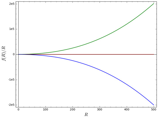
Figure 1. Plot of ${\displaystyle \frac{f(R)}{R}}$ versus R from Equation (28) for $M=1$, $w=0.14$, ${\varphi }_0=1$ and $C_1=0$ for the exponential expansion, where the green and blue lines refer to the positive and negative Lagrangian for $f(R)$, while the red line refers to the Lagrangian for general relativity (GR). One can see that the deviations from GR occur at higher-curvature regimes.

3.2. Potential $V(\varphi )$ for Exponential Expansion Models

From Equation (24), if we set

$$x=e^{-wt}$$

(29)

then we write Equation (24) by considering only the positive root, with the understanding that a similar analysis can also be performed with the negative root:

$$\varphi +{\varphi }_0=-\frac{\sqrt{2}k}{Aw}x+\frac{\sqrt{2}M}{9\sqrt{k}{A}^{3}w}{x}^3$$

(30)

The above equation has two complex solutions and one real solution, given as

$$\begin{array}{cc}\hfill x& =3^{\frac{2}{3}}A{w}^{\frac{2}{3}}{M}^{\frac{1}{3}}{\left[3\sqrt{2}Aw(\varphi +{\varphi }_0)+\sqrt{6}{\left(3w^2({\varphi }^2+{\varphi }_0^2)+6w^2\varphi {\varphi }_0+\frac{8A^2}{M}\right)}^{1/2}\right]}^{1/3}\hfill \\ & -6^{\frac{2}{3}}{A}^{\frac{1}{3}}{M}^{-\frac{2}{3}}{\left[3\sqrt{2}Aw(\varphi +{\varphi }_0)+\sqrt{6}{\left(3w^2({\varphi }^2+{\varphi }_0^2)+6w^2\varphi {\varphi }_0+\frac{8A^2}{M}\right)}^{1/2}\right]}^{-1/3}\hfill \end{array}$$

(31)

From Equation (29), we can write

$$t=-\frac{lnx}{w}$$

(32)

Here, $lnx$ is constrained to be negative such that we do not experience a negative time parameter. This is because the parameter w is a positive number by construction. The potential defined in Equation (14) reads

$$V(t)=3w^2+\frac{2}{A^2}{e}^{-wt}-\frac{M}{3A^4}{e}^{-4wt}$$

(33)

so that we have $V(\varphi )$ as

$$V(\varphi )=3w^2+\frac{2}{A^2}x-\frac{M}{3A^4}{x}^4$$

(34)

This potential and its first and second derivatives with respect to the scalar field $\varphi$ will help in constructing the slow-roll parameters from Section 5. Figure 2 below shows how the potential depends on the scalar field $\varphi$.

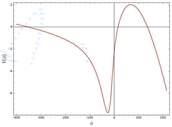
Figure 2. Plot of $V(\varphi )$ versus $\varphi$ from Equation (34) for $M=1$, $A=0.9$, $w=0.12$ and ${\varphi }_0=0.5$.

4. Linear Expansion

For linear expansion, one has a scale factor given as [24]:

$$a=At$$

(35)

where $A>0$. By replacing Equation (35) in Equation (15), we obtain

$$\dot{\varphi }=\pm {\left(\frac{2(k+A^2)}{a^2}\right)}^{1/2}{\left(1-\frac{2M}{a^2(k+A^2)}\right)}^{1/2}$$

(36)

If $\frac{2M}{a^2(k+A^2)}>1$, we would have a complex scalar field. We therefore consider the case in which $\frac{2M}{a^2(k+A^2)}<<1$. This is assumed with the fact that a is small and the constant A is large. This leads to the approximation of the above equation as

$$\dot{\varphi }=\pm \left[{\left(\frac{2(k+A^2)}{a^2}\right)}^{1/2}-\frac{\sqrt{2}M}{a^2\sqrt{(k+A^2)}}\right]$$

(37)

Replacing back the expression for the scale factor and performing integration, we have the scalar field given as

$$\varphi (t)=\pm \left[\frac{\sqrt{2(k+A^2)}}{A}ln(t)+\frac{\sqrt{2}M}{A^2\sqrt{k+A^2}t}-{\varphi }_0\right]$$

(38)

4.1. Reconstruction of $f(R)$ for Linear Inflation Models

In order to construct $f(R)$ models from scalar field formulations obtained using Equation (38), we need to have $\varphi (R)$. To achieve this, we start from the definition of the Ricci scalar given in Equation (16), so that we can write

$$R=\frac{6(A^2+k)}{A^2{t}^2}$$

(39)

From this equation, one has $t(R)$ given as

$$t(R)={\left(\frac{6(A^2+k)}{A^{2}R}\right)}^{1/2}$$

(40)

Therefore, the scalar field in Equation (38) has the form

$$\varphi (R)=\pm \left[\frac{\sqrt{2(A^2+k)}}{A}ln{\left(\frac{6(A^2+k)}{A^{2}R}\right)}^{1/2}+\frac{\sqrt{2}M}{A^2\sqrt{A^2+k}}{\left(\frac{6(A^2+k)}{A^{2}R}\right)}^{-1/2}-{\varphi }_0\right]$$

(41)

Using the definitions in Equations (18) and (19) in Equation (41), we have $f(R)$ written as

$$\begin{array}{cc}\hfill f(R)& =\pm \{\frac{\sqrt{2(A^2+k)}}{2A(A^2+k)}\left[A^{2}Rln\left(\frac{6(A^2+k)}{A^{2}R}\right)+kRln\left(\frac{6(A^2+k)}{A^{2}R}\right)+A^{2}R+kR\right]\hfill \\ & +\frac{\sqrt{12}M{R}^{3/2}}{9A(A^2+k)}-{\varphi }_{0}R\}+R+C_2\hfill \end{array}$$

(42)

where $C_2$ is a constant of integration. This Lagrangian takes a different form depending on the geometry of the spacetime, as Figure 3 depicts.

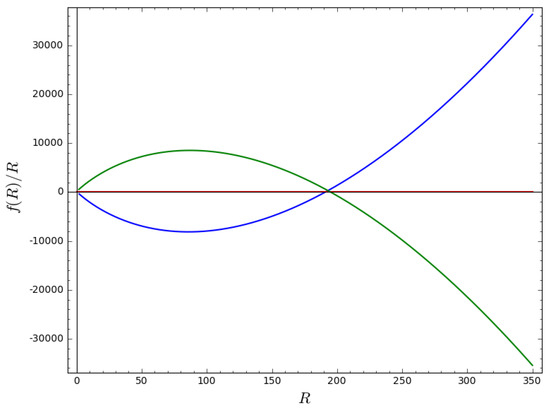
Figure 3. Plot of ${\displaystyle \frac{f(R)}{R}}$ versus R from Equation (42) for $M=1$, $C_1=-100$, ${\varphi }_0=50$, $k=1$ and $A=0.11$ for linear expansion, where the blue and green lines refer to the positive and negative Lagrangian for $f(R)$, while the red line refers to the Lagrangian for general relativity (GR).

4.2. Potential $V(\varphi )$ for Linear Inflation Models

The potential in terms of cosmic time t is given as

$$V(t)=\frac{2}{t^2}+\frac{2k}{A^2{t}^2}-\frac{M}{3A^4{t}^4}$$

(43)

We need to obtain $t(\varphi )$ in order to obtain $V(\varphi )$. From Equation (38) with the consideration of its positive root, when one considers a flat universe $(k=0)$, we have

$$t=-\frac{M}{A^3\mathbf{W}(x)}$$

(44)

where $x=-\frac{M{e}^{-\frac{\sqrt{2}(\varphi +{\varphi }_0)}{2}}}{A^3}$ and $\mathbf{W}(x)$ is Lambert’s function. The Taylor expansion for Lambert’s function is given as

$$\mathbf{W}(x)=\sum _{n=1}^{\infty }\frac{{(-n)}^{n-1}}{n!}{x}^n\approx x-x^2+\frac{3}{2}{x}^3-\frac{8}{3}{x}^4+O(x^5)$$

(45)

Thus, up to quadratic order, one has

$$\mathbf{W}(x)=-\frac{M{e}^{-\frac{\sqrt{2}(\varphi +{\varphi }_0)}{2}}}{A^3}-\frac{M^2{e}^{-\sqrt{2}(\varphi +{\varphi }_0)}}{A^6}+...$$

(46)

Replacing Equation (46) in Equation (44), we have $t(\varphi )$ as

$$t(\varphi )=\frac{M}{A^3}{\left[\frac{M{e}^{-\frac{\sqrt{2}(\varphi +{\varphi }_0)}{2}}}{A^3}+\frac{M^2{e}^{-\sqrt{2}(\varphi +{\varphi }_0)}}{A^6}\right]}^{-1}$$

(47)

Replacing $t(\varphi )$ in Equation (43), we have

$$V(\varphi )=2{\left[e^{-\frac{\sqrt{2}(\varphi +{\varphi }_0)}{2}}+\frac{M{e}^{-\sqrt{2}(\varphi +{\varphi }_{0)}}}{A^3}\right]}^2-\frac{M}{3}{\left[\frac{e^{-\frac{\sqrt{2}(\varphi +{\varphi }_0)}{2}}}{A^2}+\frac{M{e}^{-\sqrt{2}(\varphi +{\varphi }_{0)}}}{A^5}\right]}^4$$

(48)

For $k=\pm 1$, we have

$$V(t)=\frac{2(A^2\pm 1)}{A^2{t}^2}-\frac{M}{3A^4{t}^4}$$

(49)

From Equation (38), we have

$$t(\varphi )=exp\left[\frac{A({\varphi }_0+\varphi )}{\sqrt{2(A^2\pm 1)}}+\mathbf{W}(x)\right]$$

(50)

where $x=-\frac{M{e}^{-\frac{A(\varphi +{\varphi }_0)}{\sqrt{2(A^2\pm 1)}}}}{A(A^2\pm 1)}$ and the new $\mathbf{W}(x)$ is expanded as

$$\mathbf{W}(x)=-\frac{M}{A(A^2\pm 1)}{e}^{-\frac{A(\varphi +{\varphi }_0)}{\sqrt{2(A^2\pm 1)}}}-\frac{M^2}{A^2{(A^2\pm 1)}^2}{e}^{-2\frac{A(\varphi +{\varphi }_0)}{\sqrt{2(A^2\pm 1)}}}+\dots$$

(51)

Thus, one has $t(\varphi )$ given as

$$t(\varphi )=exp\left[\frac{A({\varphi }_0+\varphi )}{\sqrt{2(A^2\pm 1)}}-\frac{M}{A(A^2\pm 1)}{e}^{-\frac{A(\varphi +{\varphi }_0)}{\sqrt{2(A^2\pm 1)}}}-\frac{M^2}{A^2{(A^2\pm 1)}^2}{e}^{-2\frac{A(\varphi +{\varphi }_0)}{\sqrt{2(A^2\pm 1)}}}\right]$$

(52)

Replacing this expression for $t(\varphi )$ in Equation (49), we have

$$\begin{array}{cc}\hfill V(\varphi )& =\frac{2(A^2\pm 1)}{A^2}exp\left\{-2\left[\frac{A({\varphi }_0+\varphi )}{\sqrt{2(A^2\pm 1)}}-\frac{M}{A(A^2\pm 1)}{e}^{-\frac{A(\varphi +{\varphi }_0)}{\sqrt{2(A^2\pm 1)}}}-\frac{M^2}{A^2{(A^2\pm 1)}^2}{e}^{-2\frac{A(\varphi +{\varphi }_0)}{\sqrt{2(A^2\pm 1)}}}\right]\right\}\hfill \\ & -\frac{M}{3A^4}exp\left\{-4\left[\frac{A({\varphi }_0+\varphi )}{\sqrt{2(A^2\pm 1)}}-\frac{M}{A(A^2\pm 1)}{e}^{-\frac{A(\varphi +{\varphi }_0)}{\sqrt{2(A^2\pm 1)}}}-\frac{M^2}{A^2{(A^2\pm 1)}^2}{e}^{-2\frac{A(\varphi +{\varphi }_0)}{\sqrt{2(A^2\pm 1)}}}\right]\right\}\hfill \end{array}$$

(53)

In the following section, we apply the results obtained so far to the inflation epoch, particularly on a slow-roll approximation to see how the models respond to the inflation parameters $n_s$ and r.

5. Application to Inflation Epoch

We focus our interests on slow-roll approximations. The slow-roll approximation has the condition that the kinetic energy of the scalar field is much less than the potential [27]. This leads to two conditions as

$$\begin{array}{c}{\dot{\varphi }}^2<V(\varphi )\hfill \end{array}$$

(54)

$$\begin{array}{c}2|\ddot{\varphi }|<|V^{\prime }(\varphi )|\hfill \end{array}$$

(55)

where here, ${}^{\prime }$ indicates differentiation with respect to the scalar field $\varphi$. Then we can define two potential slow-roll parameters $ϵ(\varphi )$ and $\eta (\varphi )$ [27,28]:

$$ϵ(\varphi )=\frac{1}{2{\kappa }^2}{\left(\frac{V^{\prime }(\varphi )}{V(\varphi )}\right)}^2$$

(56)

and

$$\eta (\varphi )=\frac{1}{{\kappa }^2}\left(\frac{V^{″}(\varphi )}{V(\varphi )}\right)$$

(57)

The spectral index $n_s$ and the tensor-to-scalar ratio r are defined, respectively, as [27,28]

$$\begin{array}{c}{n}_s=1-6ϵ+2\eta \hfill \end{array}$$

(58)

$$\begin{array}{c}r=16ϵ\hfill \end{array}$$

(59)

The numerical computation of these two parameters have been performed for both the exponential and linear expansion models. The observational values of $n_s$ and r were taken from the Planck data [29].

The following Figure 4, Figure 5, Figure 6, Figure 7 and Figure 8 summarize the change of the parameters $w,A,{\varphi }_0$ and $\varphi$ to obtain both a spectral index $n_s$ and tensor-to-scalar ratio r close to the observational values for the linear law of expansion for the case in which $k=1$. Where $k=0$ and $k=-1$, one has negative and complex values for the spectral index $n_s$ and the tensor-to-scalar ratio r; this evidently rules out the corresponding $f(R)$ Lagrangian from the viable values. It is clear from the Figure 4, Figure 5, Figure 6, Figure 7 and Figure 8 presented in this work that the observational results of $n_s$ and r constrain the ranges of the parameters under variation. In Figure 4a, one can notice that r increases monotonically as a function of w until it surpasses the upper limit of the Planck data, which constrain that $r<0.11$. On the other side in Figure 4b, the spectral index decreases as w changes, and the only acceptable values can be obtained between $w=0.14$ and $w=0.177$. In Figure 5a, after $n_s$ crosses the observational value, it asymptotically varies with the increasing of A. On the other side, in Figure 5b, $n_s$ increases and saturates to a finite amplitude after it crosses the lower bound of the Planck data. In Figure 6a, the tensor-to-scalar ratio r decreases with the increasing of ${\varphi }_0$, and the values that are compatible with observation are achieved after passing ${\varphi }_0=0.42$. In Figure 6b, the spectral index $n_s$ increases with the increasing of ${\varphi }_0$ until it crosses the lower and the upper boundaries of the observational data. The same behavior is manifested in Figure 7a,b for r and $n_s$ with changing $\varphi$.

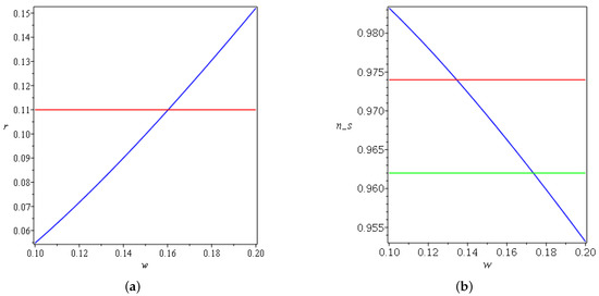
Figure 4. (a) Plot of $r(w)$ for $M=1$, $A=15$, ${\varphi }_0=1$ and $\varphi =1.2$. For exponential expansion, the red line refers to the Planck data. (b) Plot of $n_s(w)$ for $M=1$, $A=15$, ${\varphi }_0=1$ and $\varphi =1.2$. For exponential expansion, the red and green lines refer to the upper and lower bounds of Planck data, respectively.

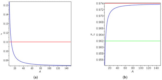
Figure 5. (a) Plot of $r(A)$ for $M=1$, $w=0.15$, ${\varphi }_0=1$ and $\varphi =1.5$. For exponential expansion, the red line refers to the Planck data. (b) Plot of $n_s(A)$ for $M=1$, $w=0.15$, ${\varphi }_0=1$ and $\varphi =1.5$. For exponential expansion, the red and green lines refer to the upper and lower bounds of Planck data, respectively.

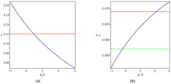
Figure 6. (a) Plot of $r({\varphi }_0)$ for $M=1$, $w=0.15$, $A=15$ and $\varphi =1.15$. For exponential expansion, the red line refers to the Planck data. (b) Plot of $n_s({\varphi }_0)$ for $M=1$, $w=0.15$, $A=15$ and $\varphi =1.15$. For exponential expansion, the red and green lines refer to the upper and lower bounds of Planck data, respectively.

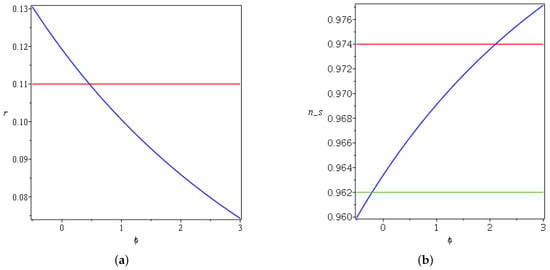
Figure 7. (a) Plot of $r(\varphi )$ for $M=1$, $w=0.15$, $A=15$ and ${\varphi }_0=1.15$. For exponential expansion, the red line refers to the Planck data. (b) Plot of $n_s(\varphi )$ for $M=1$, $w=0.15$, $A=15$ and ${\varphi }_0=1.15$. For exponential expansion, the red and green lines refer to the upper and lower bounds of Planck data, respectively.

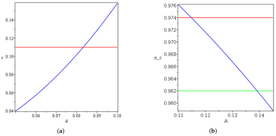
Figure 8. (a) Plot of $r(A)$ for $M=1$, ${\varphi }_0=750$ and $\varphi =1.05$. For linear expansion, the red line refers to the Planck data. (b) Plot of $n_s(A)$ for $M=1$, ${\varphi }_0=750$ and $\varphi =1.05$. For linear expansion, the red and green lines refer to the upper and lower bounds of Planck data, respectively.

For the linear expansion model, Figure 8a,b shows how r and $n_s$ change as a function of A. The tensor-to-scalar ratio increases as a function of A, and $n_s$ decreases as a function of A. This makes $n_s$ cross the upper bound first, and later it crosses the lower bound.

6. Conclusions

In this paper, we studied cosmological fluid systems composed of radiation and a scalar field and with predetermined inflationary expansion scenarios of the FLRW background spacetime. Using the scalar field as the extra degree of freedom that appears in generic $f(R)$-gravity models, we reconstructed $f(R)$ Lagrangians and the corresponding potentials for the scalar field. The reconstructed $f(R)$ actions have GR and $\Lambda$CDM actions as limiting cases. We applied the results to slow-roll approximations to show that in fact, the parameters that are involved in the Lagrangian reconstruction can be constrained by observational data.

References

- Guth, A.H. Inflationary universe: A possible solution to the horizon and flatness problems. Phys. Rev. D 1981, 23, 347–356. [Google Scholar]
- Starobinsky, A.A. A new type of isotropic cosmological models without singularity. Phys. Lett. B 1980, 91, 99–102. [Google Scholar]
- Barrow, J.D.; Paliathanasis, A. Reconstructions of the dark-energy equation of state and the inflationary potential. arXiv, 2016; arXiv:1611.06680. [Google Scholar]
- Nojiri, S.; Odintsov, S.D.; Oikonomou, V.K. Modified Gravity Theories on a Nutshell: Inflation, Bounce and Late-time Evolution. Phys. Rept. 2017, 692, 1–104. [Google Scholar]
- Nojiri, S.; Odintsov, S.D. Modified gravity with negative and positive powers of curvature: Unification of inflation and cosmic acceleration. Phys. Rev. D 2003, 68, 123512. [Google Scholar]
- Nojiri, S.; Odintsov, S.D. Unifying inflation with ΛCDM epoch in modified f (R) gravity consistent with Solar System tests. Phys. Lett. B 2007, 657, 238–245. [Google Scholar]
- Nojiri, S.; Odintsov, S.D. Future evolution and finite-time singularities in f (R) gravity unifying inflation and cosmic acceleration. Phys. Rev. D 2008, 78, 046006. [Google Scholar]
- Nojiri, S.; Odintsov, S.D. Unified cosmic history in modified gravity: From f (R) theory to Lorentz non-invariant models. Phys. Rep. 2011, 505, 59–144. [Google Scholar]
- Bamba, K.; Nojiri, S.; Odintsov, S.D.; Sáez-Gómez, D. Inflationary universe from perfect fluid and f (R) gravity and its comparison with observational data. Phys. Rev. D 2014, 90, 124061. [Google Scholar]
- Amin, M.; Khalil, S.; Salah, M. A viable logarithmic f (R) model for inflation. J. Cosmol. Astropart. Phys. 2016, 2016, 043. [Google Scholar]
- Li, B.; Barrow, J.D. Cosmology of f (R) gravity in the metric variational approach. Phys. Rev. D 2007, 75, 084010. [Google Scholar] [CrossRef]
- Chakraborty, S.; SenGupta, S. Solving higher curvature gravity theories. Eur. Phys. J. C 2016, 76, 552. [Google Scholar] [CrossRef]
- Sáez-Gómez, D. Modified f (R) gravity from scalar-tensor theory and inhomogeneous EoS dark energy. Gen. Relativ. Gravit. 2009, 41, 1527–1538. [Google Scholar] [CrossRef]
- Nojiri, S.; Odintsov, S.D.; Sáez-Gómez, D. Cosmological reconstruction of realistic modified f (R) gravities. Phys. Lett. B 2009, 681, 74–80. [Google Scholar] [CrossRef]
- Ntahompagaze, J.; Abebe, A.; Mbonye, M. On f (R) gravity in scalar-tensor theories. Int. J. Geom. Methods Mod. Phys. 2017, 14, 1750107. [Google Scholar] [CrossRef]
- Sami, H.; Namane, N.; Ntahompagaze, J.; Elmardi, M.; Abebe, A. Reconstructing f (R) Gravity from a Chaplygin Scalar Field in de Sitter Spacetimes. arXiv, 2017; arXiv:1706.07790. [Google Scholar]
- Faraoni, V. De Sitter space and the equivalence between f (R) and scalar-tensor gravity. Phys. Rev. D 2007, 75, 067302. [Google Scholar] [CrossRef]
- Paliathanasis, A. f (R)-gravity from Killing tensors. Class. Quantum Gravity 2016, 33, 075012. [Google Scholar] [CrossRef]
- Paliathanasis, A.; Tsamparlis, M.; Basilakos, S. Constraints and analytical solutions of f (R) theories of gravity using Noether symmetries. Phys. Rev. D 2011, 84, 123514. [Google Scholar] [CrossRef]
- Guth, A.H. Inflation. Proc. Natl. Acad. Sci. USA 1993, 90, 4871–4877. [Google Scholar] [CrossRef] [PubMed]
- Linde, A. Inflationary cosmology after Planck. In Post-Planck Cosmology: Lecture Notes of the Les Houches Summer School: Volume 100, July 2013; Oxford University Press: Oxford, UK, 2015; Volume 100, pp. 231–303. [Google Scholar]
- Bassett, B.A.; Tsujikawa, S.; Wands, D. Inflation dynamics and reheating. Rev. Mod. Phys. 2006, 78, 537–589. [Google Scholar] [CrossRef]
- Huang, Q.G. A polynomial f (R) inflation model. J. Cosmol. Astropart. Phys. 2014, 2014, 035. [Google Scholar] [CrossRef]
- Ellis, G.; Madsen, M. Exact scalar field cosmologies. Class. Quantum Gravity 1991, 8, 667–676. [Google Scholar] [CrossRef]
- Gorini, V.; Kamenshchik, A.; Moschella, U.; Pasquier, V. The Chaplygin Gas as a Model for Dark Energy. In Proceedings of the Tenth Marcel Grossmann Meeting, Rio de Janeiro, Brazil, 16–18 July 2003; pp. 840–859. [Google Scholar]
- Frolov, A.V. Singularity problem with f (R) models for dark energy. Phys. Rev. Lett. 2008, 101, 061103. [Google Scholar] [CrossRef] [PubMed]
- Liddle, A.R.; Parsons, P.; Barrow, J.D. Formalizing the slow-roll approximation in inflation. Phys. Rev. D 1994, 50, 7222–7232. [Google Scholar] [CrossRef]
- Liddle, A.R.; Lyth, D.H. COBE, gravitational waves, inflation and extended inflation. Phys. Lett. B 1992, 291, 391–398. [Google Scholar] [CrossRef]
- Ade, P.; Aghanim, N.; Arnaud, M.; Arroja, F.; Ashdown, M.; Aumont, J.; Baccigalupi, C.; Ballardini, M.; Banday, A.; Barreiro, R.; et al. Planck 2015 results-XX. Constraints on inflation. Astron. Astrophys. 2016, 594, A20. [Google Scholar]
© 2017 by the authors. Licensee MDPI, Basel, Switzerland. This article is an open access article distributed under the terms and conditions of the Creative Commons Attribution (CC BY) license (http://creativecommons.org/licenses/by/4.0/).