Abstract
The electron temperature (Te) behavior at small scales (both spatial and temporal) in the topside ionosphere is investigated through in situ observations collected by Langmuir Probes on-board the European Space Agency Swarm satellites from the beginning of 2014 to the end of 2020. Te observations are employed to calculate the Rate Of change of electron TEmperature Index (ROTEI), which represents the standard deviation of the Te time derivative calculated over a window of fixed width. As a consequence, ROTEI provides a description of the small-scale variations of Te along the Swarm satellites orbit. The extension of the dataset and the orbital configuration of the Swarm satellites allowed us to perform a statistical analysis of ROTEI to unveil its mean spatial, diurnal, seasonal, and solar activity variations. The main ROTEI statistical trends are presented and discussed in the light of the current knowledge of the phenomena affecting the distribution and dynamics of the ionospheric plasma, which play a key role in triggering Te small-scale variations. The appearance of unexpected high values of ROTEI at mid and low latitudes for specific magnetic local time sectors is revealed and discussed in association with the presence of Te spikes recorded by Swarm satellites under very specific conditions.
1. Introduction
The topside ionosphere is an environment characterized by very complex dynamics due to the interplay between solar radiation, the flux of particles embedded in the solar wind, the configuration of the Earth’s magnetic field, the distribution and dynamic properties of the different chemical species in the Earth’s atmosphere, and the interaction with the neutral atmosphere dynamics [1,2,3]. All of this influences the plasma distribution and dynamics of the topside ionosphere, which in turn exhibits peculiar spatial, diurnal, seasonal, solar, and magnetic activity variations on very different spatial and temporal scales [4,5].
Over the years, most attention has been focused on the description of the topside ionosphere electron density (Ne) at both large and small spatial and time scales. Large scales describe the median statistical behavior of Ne, i.e., the main spatial, diurnal, seasonal, and solar activity variabilities. Ne behavior at these scales is well described by empirical climatological ionospheric models like the International Reference Ionosphere (IRI, [6]). Differently, small scales describe the large day-to-day variability of the ionosphere, like for example that exhibited during geomagnetic storms [7,8]. Small-scale irregularities in Ne can be investigated through the calculation of ionospheric indices based on local in situ Ne observations from Langmuir Probes (LP) on-board low-Earth-orbit (LEO) satellites, or based on nonlocal total electron content (TEC) observations from ground-based or satellite-based Global Navigation Satellite System (GNSS) receivers. The ionospheric index named Rate Of change of electron Density Index (RODI, [9]) is derived from LPs in situ Ne observations, while the Rate Of change of Total electron content Index (ROTI, [10]) is calculated from nonlocal TEC observations. These two indices allowed identifying a large spectrum of Ne irregularities ranging from meters to hundreds of kilometers, particularly affecting the high [9,11,12,13,14] and low [15,16,17,18] latitudes.
On the contrary, as far as we know, electron temperature (Te) small-scale variations have not been extensively investigated yet, despite their possibly crucial role in the characterization of the energy budget of ionospheric plasma, especially at auroral latitudes, and in the occurrence of plasma irregularities [19,20,21,22,23,24]. This is why Pignalberi [25] has recently proposed a new ionospheric index named the Rate Of change of electron TEmperature Index (ROTEI) for the characterization of the in situ Te small-scale variability. ROTEI shares the same mathematical framework of the best known RODI; as a consequence, it inherits the RODI features and skills. In the Topside Ionosphere Turbulence Indices with Python (TITIPy, https://github.com/pignalberi/TITIPy, accessed on 3 January 2021, [25]) tool, ROTEI is derived from Te values measured at 2 Hz rate by LPs on-board the European Space Agency (ESA) Swarm satellites constellation [26]. After defining ROTEI and describing the corresponding calculation algorithm, Pignalberi [25] provided a first example of ROTEI application based on Swarm A data recorded during a period encompassing the St. Patrick’s day geomagnetic storm that happened on 17 March 2015. From that very preliminary analysis it emerged that high ROTEI values characterize the auroral latitudes, and that during geomagnetic disturbed conditions the regions characterized by high ROTEI values expand equatorward while ROTEI increases in magnitude [25].
The orbital configuration and the instrumentation on-board the three Swarm satellites [27] guarantee an accurate determination of ROTEI on a global basis, for different magnetic local times (MLT), seasons, and for the different solar activity levels covered since Swarm satellites were deployed in orbit at the end of 2013. Taking advantage of seven years (1 January 2014 to 31 December 2020) of Swarm Te observations, we investigated the statistical behavior of ROTEI in order to characterize the main features of Te small-scale variations in the topside ionosphere. We discussed the ROTEI spatial distribution on a global scale, its diurnal and seasonal trends, and its variations induced by solar activity. Moreover, the appearance of very high ROTEI values at mid and low latitudes for specific MLT sectors was investigated and related to the presence of Te recorded by Swarm LPs.
2. Data and Method
2.1. In Situ Electron Temperature Data by ESA Swarm Langmuir Probes
Swarm is an ESA constellation of three LEO satellites in operation since December 2013 [26]. The three satellites (conventionally named A, B, and C) were deployed in a circular near-polar orbit with the following orbital configurations: Swarm A and C fly in-tandem with an orbit inclination of 87.35° at an initial altitude of about 460 km, while Swarm B has an orbit inclination of 87.75° and an initial altitude of about 510 km. As a consequence, Swarm satellites take about 130–140 days to cover all MLTs.
Swarm satellites carry LPs providing in situ Ne and Te observations at 2 Hz rate [28,29]. Swarm LPs data are available at ftp://swarm-diss.eo.esa.int (accessed on 14 April 2021). In this work, we used 2 Hz Te observations from LPs on-board Swarm satellites recorded from 1 January 2014 to 31 December 2020 to compute ROTEI. However, in this paper we show only the results from the Swarm B satellite, those from Swarm A and C being consistently similar. Specifically, we considered only data recorded with LPs in “High-Gain” mode (by applying the flags described in https://earth.esa.int/documents/10174/1514862/Swarm_L1b_Product_Definition%20 (accessed on 14 April 2021)) to maximize the reliability of the dataset.
2.2. ROTEI Calculation
Time series of ROTEI at 2 Hz rate for the Swarm B dataset were calculated by running the TITIPy tool [25] available at https://github.com/pignalberi/TITIPy (accessed on 3 January 2021).
ROTEI is the standard deviation of the Te time derivative calculated in a window of fixed width sliding along the time series [25]:
where ROTE (Rate Of change of electron TEmperature) is the time derivative of Te recorded at time t:
and is the arithmetic mean of ROTE values in the sliding window:
In Equations (1)–(3), δt is the time step of the Te time series, Δt is the width of the sliding window, and N is the number of Te values falling in the window (which in turn depends on δt and Δt according to N = Δt/δt + 1).
ROTEI was calculated with the default TITIPy specifications [25], namely δt = 0.5 s (since Te data are at 2 Hz rate), Δt = 10 s, then N = 21. For more information on the ROTEI calculation algorithm by TITIPy refer to [25].
An example of ROTE and ROTEI values obtained from Te observed by Swarm B is presented in Figure 1. In the first two rows of this figure, we report the Te values recorded by Swarm B on 5 January 2018 at 13:53:04 Universal Time (UT) (equator crossing point, ascending semiorbit) in the first column, and the corresponding ROTE and ROTEI in the second and third columns, respectively. Data are represented both in geographic maps (first row plots) and as a function of latitude (second and third row plots). Figure 1 clearly displays the ability of both ROTE and ROTEI in catching Te small-scale variations. In fact, between about 50°N and 85°N, large variations in the magnitude of Te cause the steep increase of ROTE and ROTEI (consider that ROTE and ROTEI are represented in a logarithmic scale).
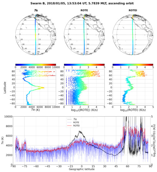
Figure 1.
Te (first column), ROTE (second column), and ROTEI (third column) values recorded by Swarm B on 5 January 2018 at 13:53:04 UT (equator crossing point), ascending semiorbit. Data are represented in geographic maps (first row plots), and as separated (second row plots) and superposed time series (third row plots). In the first and second row plots, data are represented as scatter points whose color identifies the corresponding magnitude (ROTE and ROTEI values are in logarithmic scale). In the bottom plot, data are represented as curves of different colors: black for Te, blue for ROTE, and red for ROTEI.
Generally speaking, ROTEI is more effective than ROTE in describing Te variations because it is calculated on a sliding window whose width has been chosen to accurately represent a range of scales spanning from few to hundreds of kilometers. This range of scales has been widely investigated in the past years, in particular for what concerns Ne irregularities; for example, ([13,14,18] and references therein) showed how irregularities occurring at these scales are intimately related to turbulent phenomena, at both low and high latitudes. Due to its mathematical definition, ROTEI describes the variability of Te at the scale of the window used for its calculation and is unaffected by larger-scale Te variations; this is well visible in Figure 1 by comparing the Te and ROTEI trends at low latitudes with the corresponding ones at Northern high latitudes. Likewise, ROTEI values are much lower where Te varies slowly (like at Southern mid latitudes in Figure 1); in fact, Figure 1 shows a difference of more than two orders of magnitude between the lowest and highest ROTEI values.
3. Statistical Trends of ROTEI in the Topside Ionosphere
Spatial, diurnal, seasonal, and solar activity trends of binned ROTEI values were obtained from Swarm B Te observations at 2 Hz from 2014 to 2020. The mean value was considered as the representative one within each bin. Since the plasma distribution and dynamics in the topside ionosphere is strongly affected by the configuration of the Earth’s magnetic field, we binned ROTEI as a function of the Quasi-Dipole magnetic latitude (QD, [30]), and MLT. Specifically, data were binned in 2.5° wide bins in QD latitude, and fifteen-minute wide bins in MLT.
3.1. On the ROTEI Diurnal and Seasonal Trends
The seasonal trend is investigated by splitting data in four periods centered at solstices and equinoxes based on the day of the year (doy): March equinox, 35 ≤ doy ≤ 125; June solstice, 126 ≤ doy ≤ 217; September equinox, 218 ≤ doy ≤ 309; December solstice, doy ≤ 34 OR doy ≥ 310. The mean value of each bin was calculated to represent the main statistical behavior of ROTEI. In each bin, the number of ROTEI values on which the mean values were calculated ranges between 102 and 104.5 with the bulk of bins containing about 104 values. The less populated bins are those characterizing the low latitudes in the diurnal sector for years of high solar activity (2014 and 2015), due to the use of only “High-Gain” LPs data (see Section 2.1). The mean values were calculated only for bins with at least 10 values.
In Figure 2, ROTEI mean values are represented as polar projection with MLT and the QD latitude being respectively the azimuth and radius, for the Northern (NH, first row plots) and Southern (SH, second row plots) hemispheres. The different local seasons are represented in different columns: spring in the first column plots, i.e., March equinox for NH and September equinox for SH; summer in the second column plots, i.e., June solstice for NH and December solstice for SH; autumn in the third column plots, i.e., September equinox for NH and March equinox for SH; winter in the fourth column plots, i.e., December solstice for NH and June solstice for SH. The scale is the same across all plots and is logarithmic to best represent the large variability in magnitude exhibited by ROTEI for different latitudes and MLTs.
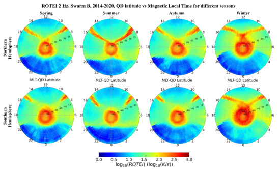
Figure 2.
Statistical spatial, diurnal, and seasonal trends of ROTEI obtained from Te data measured by Swarm B from 2014 to 2020. Those represented are binned mean values in QD magnetic coordinates in polar projection; the bin size is (azimuth) 15 minutes in MLT, (radius) 2.5° in QD latitude. First row for the Northern hemisphere, second row for the Southern hemisphere. The first column plots are for the spring season, the second column for summer, the third column for autumn, and the fourth column for winter.
Figure 2 highlights the spatial, diurnal, and seasonal features of ROTEI mean values. In more detail:
- a)
- ROTEI exhibits a well-marked latitudinal dependence. Auroral latitudes are characterized by the highest ROTEI values (in the range between 102 and 103 K/s), while non-auroral ones experience the lowest values of ROTEI except for very specific MLTs;
- b)
- limited to the MLT sectors around 9:00 and 15:00, the mid and low latitudes are characterized by the presence of very high ROTEI values that depart from the equator and merge with the high ROTEI values at auroral latitudes. Specifically, at the equator such high ROTEI values are always located at 9:00 and 15:00 MLT, but rising towards mid latitudes their shape can change with the season and these very high ROTEI values can be found also at different MLTs. In particular, this is the case for the winter season, where the two strips of high ROTEI values start at the equator at 9:00 and 15:00 MLT, but then merge with each other at 12:00 MLT at mid latitudes;
- c)
- at mid and low latitudes, ROTEI is higher during daytime (between 10 and 101.75 K/s) than at nighttime (between 100.25 and 101.25 K/s). The two different behaviors are well separated at MLTs characterized by the solar terminator passage (both at sunrise and sunset), the shape of which changes with the season due to the different solar illumination conditions;
- d)
- the seasonal dependence is limited to the auroral latitudes and to MLTs 9:00 and 15:00 at mid and low latitudes. In fact, the high latitudes exhibit a large seasonal variation, with highest ROTEI in winter and lowest in summer, which is opposite to the solar illumination conditions. Moreover, in local winter, the high-latitude region characterized by the highest ROTEI expands towards mid latitudes by reaching about 55–60° of QD latitude in both hemispheres, compared to about 65–75° in summer, and 60–70° at equinoctial seasons. At high latitudes, for all seasons, the latitudinal extension of high ROTEI values is more marked at nighttime, where lower latitudes are reached, compared to daytime. Somewhat expected is the fact that equinoctial seasons are very similar at all latitudes and MLTs.
The presence of very high ROTEI values at high latitudes finds its explanation in the phenomena affecting the auroral oval. At high latitudes, ROTEI highest values draw a ring around the magnetic poles and are elongated towards lower latitudes in the nighttime sector. Indeed, auroral latitudes are characterized by particle precipitation causing the increase of Te in the topside ionosphere through Joule heating. A recent work by [31] investigated the seasonal behavior of the electrical conductivity parallel to the Earth’s magnetic field, by using only plasma data (Ne and Te) from Swarm A spacecraft. Although the parallel conductivity also shows a slight dependence on Ne, the main contributor to it remains Te (see Equation (6) in [31]). In their work, the authors of [31] estimated the contribution to conductivity from particle precipitation by subtracting from the overall conductivity that inferred from Ne and Te modeled by IRI [6]. They found a remarkable variability with season of the parallel conductivity (and, to a large extent, of Te), showing that the effect of precipitation increases the parallel conductivity (and Te) especially in the nightside and approaching the border of the auroral oval at ± 60° QD latitude, and in the region of the dayside cusp, and this effect is stronger in winter than in summer and at equinoxes.
Differently from parallel conductivity and Te, the maps in Figure 2 show an almost homogeneous enhancement of ROTEI throughout the auroral oval regions, with the exception of a maximum in the cusps, that could be directly associated with the effect of particle precipitation. Moreover, the area of high ROTEI at high latitudes seems to considerably expand to lower latitudes in winter, especially in the Southern hemisphere. This implies that the distributions of the small-scale Te gradients at high latitudes only broadly match the patterns of Te itself, and the occurrence of Te variations seems rather to be a ubiquitous phenomenon of the auroral regions, possibly related to the presence of horizontal currents and zonal electric fields which strongly act on plasma dynamics almost all the time.
It is also worth noting that ROTEI exhibits very peculiar features under different solar illumination conditions. Firstly, while at mid and low latitudes the highest (lowest) ROTEI values observed at daytime (nighttime) suggest a strong coupling with the sunlit conditions, at high latitudes the situation is very different. There, the diurnal trend of ROTEI does not follow the solar illumination conditions and, more importantly, the seasonal trend shows the highest values of ROTEI in winter and the lowest in summer, as already pointed out above. Te gradients are present at all MLTs and QD latitudes due to the energy deposited via the joint action of solar illumination on the dayside, particle precipitation on both the dayside (in correspondence of the cusp and at lower latitudes in the prenoon sector) and the nightside (especially in correspondence with the boundary between Region 2 and the ionospheric trough), and convective motions of plasma through neutrals in the polar cap regions (see, e.g., [32,33]). Above around ±60° of QD latitude, i.e., at auroral latitudes, the strongest Te gradients observed point out the steeper small-scale variation of Te, which is mainly due to particle precipitation, which is a manifestation of the magnetosphere-ionosphere coupling and plays a fundamental role in the exchange of energy and momentum. In more detail, on the dayside, at QD latitudes of around ±80°, an enhancement of Te is expected around noon [34] and at slightly lower latitudes in the prenoon sector [21] due to an intense electron precipitation from the (open) magnetosphere [35]. On the nightside, an intense particle precipitation is observed especially in the equatorward part of the Region 2 [36], corresponding to field-aligned currents flowing from the magnetosphere to the ionosphere. The energy peak of precipitating particles is observed in correspondence with the position of the main ionospheric trough, where Te increases due to both the energy exchanges with the nightside magnetosphere and the depletion of Ne [37]. This behavior also affects Te gradients, as we can see from Figure 2. The net result is an enhancement of ROTEI (and, thus, of Te gradients) at almost all MLTs. This enhancement of Te is particularly pronounced during the nightside winter, when the contribution of particle precipitation to Te is dominant due to both the increased energy of the precipitating particles and the decreased Ne that prevents the slowing of precipitating particles via collisional cooling [38]. We also notice that the regions of enhanced Te gradients on both dayside and nightside are located more poleward during the summer than during the winter. This is consistent with the findings of the authors of [39,40], who discussed this observation in terms of the shift of field-aligned current systems. We remark that despite a reduction of precipitation events is expected at very high latitudes on the dayside winter with respect to the dayside summer due to the reduced electron flux number [41], when looking at local small-scale Te gradients pointed out by ROTEI, an increase during winter emerges also in the dayside. This suggests that while Te during summer is higher than in winter on the dayside polar regions, Te gradients undergo the opposite behavior, and are higher on the dayside in winter than in summer.
The presence of very high ROTEI values at mid and low latitudes for the MLT sectors around 9:00 and 15:00 is hard to explain. In fact, for these MLTs and locations, Te in the topside ionosphere does not exhibit any specific large-scale feature that could be readily connected with these very high ROTEI values. Moreover, we have to consider that in Figure 2 we represented the mean ROTEI values in the bin; as a consequence, these extremely high ROTEI values are not sporadic but represent the bulk of the data for the interested bins. This is why, in Section 4, we look for a possible correlation between high ROTEI values and spikes in the Te values recorded by Swarm LPs, whose presence is known to the Swarm community.
3.2. On the ROTEI Solar Activity Variation
To study the solar activity impact on ROTEI, we calculated ROTEI maps in polar projection (like we did for Figure 2 plots) for each year. Our dataset comprises data collected by Swarm B satellite from 2014 to 2020, i.e., from maximum to minimum solar activity level of the last solar cycle.
In Figure 3, ROTEI mean values are represented in polar projection (MLT vs. QD latitude), for the NH (first row plots) and the SH (second row plots), from 2014 to 2020 (from left to right). To highlight the variation of solar activity, the third row plot represents the daily F10.7 solar index time series [42] and the corresponding 81 day running mean (F10.781), which best represents the long-term solar activity variation. As highlighted by F10.781 values, the year 2014 encompasses the maximum of the last solar cycle, the years 2015–2017 the descending part of the solar cycle, and the years 2018–2020 the quite-long-lasting solar minimum.
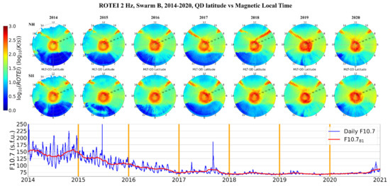
Figure 3.
Statistical annual trends of ROTEI obtained from Te data measured by Swarm B from 2014 to 2020. Those represented are binned mean values in QD magnetic coordinates in polar projection; the bin size is (azimuth) 15 minutes in MLT, (radius) 2.5° in QD latitude. First row for the Northern hemisphere (NH), second row for the Southern hemisphere (SH). In the third row the time series of the F10.7 solar index (blue curve) and the corresponding 81 day running mean (F10.781, red curve).
Overall, ROTEI exhibits a faint solar activity dependence by showing higher values during low solar activity. Specifically, at mid and low latitudes, ROTEI increases from 2014 to 2020; this is particularly evident at nighttime and dawn hours. In these MLT sectors, the highest ROTEI are recorded for the years 2019 and 2020. Moreover, at high latitudes a slight increase of ROTEI is visible. Compared to the spatial, diurnal, and seasonal variations, solar activity is a source of Te variations that is of second order importance. However, in this comparison we should keep in mind that the last solar cycle was very weak if compared to the previous ones.
Unfortunately, despite the fact that several papers have pointed out the dependence of Te on altitude, latitude, local time, season, geomagnetic and solar activity mainly with radar facilities, to our knowledge very few statistical characterizations of small-scale Te variations exist in the literature. For example, [43] found that Te at mid latitudes is slightly higher during low solar activity than during high solar activity, especially in summer and at equinoxes. [44] found that Te increases with solar activity of a few degrees K per sfu. [45] found that Te increases during solar flares on the dayside from 1.3 to ~2 times the value during quiet periods. In this respect, the observed ROTEI behavior seems to agree with those pictures. In a very recent work, [46] investigated the statistical behavior of the electrical conductivity parallel to the Earth’s magnetic field as a function of solar and geomagnetic activity by using the same approach as the authors of [31]. They found that the parallel conductivity (and so, to a larger extent, Te) generally increases in the dayside, and decreases in the nightside with solar activity. The explanation given by the authors of [46] to this effect is the following: during periods of high solar activity, the increase of Te in the nightside due to particle precipitation is balanced by a cooling due to collisions with ions, while the reduction of the EUV flux during low solar activity periods causes a strong reduction of both ion and electron densities, so also reducing the electron cooling; therefore, as a net result, a higher Te (and a higher parallel conductivity) is observed in the nightside during low solar activity. This is also observed in the ROTEI maps of Figure 3, especially when looking at the maps of 2019 and 2020, which correspond to the minimum of the last solar cycle.
4. Investigating the Correlation between High ROTEI Values and Electron Temperature Spikes
The investigation of Swarm LPs data has revealed the presence of spikes in Te, i.e., abrupt increases above the background state lasting for a few seconds. Such Te spikes are known to the Swarm community and the interpretation of their occurrence and distribution is still ongoing and matter of debate (see, e.g., https://earth.esa.int/eogateway/documents/20142/37627/swarm-preliminary-plasma-dataset-user-note.pdf/6e8c356f-16d9-5145-1cc9-a9c5736653ab, accessed on 9 April 2021). At least part of the features exhibited by Te spikes can be associated with physical phenomena happening at auroral latitudes as, for example, intense subauroral ion drifts [19]; while for other features it is difficult to find a physical reason, and the contamination due to instrumental/environmental effects is also taken into consideration as a possible explanation.
We tried to correlate the distribution and magnitude of ROTEI with the occurrence of spikes in the Swarm B Te dataset. We consider as spikes those Te observations greater than 6000 K. To properly compare ROTEI and Te spikes, from the Swarm B dataset (see Section 2.1) we selected all the observations for which Te ≥ 6000 K and then binned them like we did for ROTEI (see Section 3.1) to reveal their spatial, diurnal, and seasonal occurrence. In Figure 4, to facilitate the visual comparison between the distribution and magnitude of both ROTEI and Te spikes, ROTEI mean values (the same as Figure 2), the number of occurrences of Te spikes in the bin, and Te spikes percentage occurrence in the bin are shown side-by-side as polar plots in MLT vs. QD latitude, for the four seasons and for both hemispheres. Te spike percentage occurrences in the bin are calculated by normalizing the number of Te spikes in the bin to the total number of Te observations in the same bin.
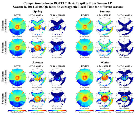
Figure 4.
Comparison between ROTEI values shown in Figure 2 and Te spikes (Te ≥ 6000 K) recorded by Swarm B from 2014 to 2020, for each season and for both hemispheres. Each panel contains the ROTEI mean values (first and fourth columns), the number of values satisfying the condition Te ≥ 6000 K in the bin (second and fifth columns), and the percentage occurrence of Te spikes in the bin (third and sixth columns). Data are binned in QD magnetic coordinates in polar projection; the bin size is (azimuth) 15 minutes in MLT, (radius) 2.5° in QD latitude, for the Northern and Southern hemispheres. Clockwise from the upper left panel, the spring, summer, winter, and autumn seasons are represented.
The comparison between ROTEI and Te spikes in Figure 4 reveals several interesting similarities between them. Specifically:
- a)
- the spatial distribution of Te spikes matches quite well with that of high ROTEI values. Te spikes are present at high latitudes all over the day, at mid and low latitudes for the MLT sectors around 9:00 and 15:00, and around the equator in the concomitance of the Te pre-sunrise peak. This matching also suggests that the Te spikes found occurred on small scales, as they correspond to small-scale Te gradients pointed out by high ROTEI values;
- b)
- Te spikes maximize in the winter season, are minimum in summer, and show an intermediate behavior at both equinoxes (that are very similar to each other). The seasonal variation in the number of spikes is very remarkable at high latitudes whose number can reach up to 40% of the Te total observations in winter in the Southern hemisphere, while they are below 10% in summer, and can reach up to 20% in the equinoxes at nighttime. The seasonal variation is similar to that exhibited by ROTEI values;
- c)
- the Te spikes’ spatial distribution shows an asymmetry between hemispheres (not present in ROTEI). In particular, at high latitudes, in the NH spikes are more concentrated in the nighttime sector, while in the SH their diurnal distribution is more homogeneous. Moreover, the number of Te spikes is much larger in the SH than in the NH;
- d)
- it is very remarkable how the spatial distribution of Te spikes at mid and low latitudes for the MLT sectors around 9:00 and 15:00 matches that of high ROTEI values. In fact, seasonal variability of Te spikes matches very well that of ROTEI at both mid and low latitudes.
According to Figure 4, high ROTEI values and Te spikes exhibit very similar spatial, diurnal, and seasonal patterns. However, while for high latitudes the high percentage occurrence of Te spikes suggests a strong link with high ROTEI values, at mid and low latitudes for the MLT sectors around 9:00 and 15:00 the relatively low number of Te spikes (less than 5%) can hardly explain the occurrence of very high ROTEI values. In fact, ROTEI polar plots represent the mean value of ROTEI within each bin. The only presence of sporadic Te spikes at mid and low latitudes is not enough to explain the high ROTEI there observed.
To further investigate the possible link between high ROTEI values at mid and low latitudes around 9:00 and 15:00 MLT and the corresponding Te spikes, we selected all the Swarm B semiorbits (both ascending and descending) from 2014 to 2020 for which at least one Te spike is present for |QD latitude| ≤ 45° and 8:00 ≤ MLT ≤ 16:00, and plotted Te, ROTE, and ROTEI time series to visually check their behavior under these conditions. As an example, in Figure 5 we show these three quantities as a function of geographic latitude for three consecutive Swarm B descending semiorbits on 24th June 2017 at around 10:00 MLT (shown in three different plots), for which Te spikes are present at SH mid latitudes. In all the three plots on the left of Figure 5 a cluster of Te spikes between -40° and -20° geographic latitude is present; each cluster is composed of a few Te spikes (between 3 and 7), but each spike is surrounded by highly oscillating Te values (like highlighted in the inset on the right of Figure 5) that cause the increase of both ROTE and ROTEI. In fact, we can see that ROTEI maximizes in concomitance of Te spikes but very high ROTEI values are also present around the spikes due to the very high variability that Te exhibits around them. The cases shown in Figure 5 are very representative of the Te spikes morphology and Te variability at mid and low latitudes. ROTEI keeps values 1–2 orders of magnitude higher with respect to its background level in rather wide latitude ranges encompassing the actual spikes’ occurrence. This behavior is not sporadic and casual, but it happens in a systematic way in these MLT sectors. This is why the presence of steep Te variations, whose origin is still not unambiguously known and under investigation, is the most probable explanation of the high ROTEI values at mid and low latitudes around 9:00 and 15:00 MLT. A similar behavior is also characteristic of the high latitudes, as highlighted in Figure 5, and certainly plays a role in the explanation of the high ROTEI values at high latitudes (see Figure 4).
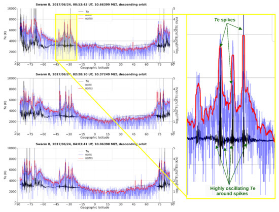
Figure 5.
Te (in black), ROTE (in blue), and ROTEI (in red) time series for three consecutive descending semiorbits (from top to bottom panels), as recorded by Swarm B on 24 June 2017. The date, UT, and MLT of the equator crossing point are given on the top of each plot.
5. Conclusions
In this work, we highlighted the statistical behavior of ROTEI to characterize the mean spatial, diurnal, seasonal, and solar activity variations exhibited by small-scale Te variations in the topside ionosphere. Taking advantage of both seven years (from 2014 to 2020) of in situ Te observations at 2 Hz from LPs on-board Swarm B satellite, and the TITIPy tool [25], we calculated time series of ROTEI and binned them as a function of the QD latitude, MLT, season, and year, to unveil the corresponding behavior for different conditions.
The most remarkable outcomes of the study are:
- 1)
- the presence of very high ROTEI values at high latitudes all over the day, and at mid and low latitudes for the MLT sectors around 9:00 and 15:00;
- 2)
- ROTEI exhibits a distinct day/night diurnal trend at low and mid latitudes, which is instead quite negligible at high latitudes;
- 3)
- high latitudes exhibit a large seasonal variation with the highest ROTEI values in winter and lowest in summer, while at mid and low latitudes the seasonal dependence is weaker;
- 4)
- ROTEI exhibits a faint solar activity dependence with slightly higher values at low solar activity.
To explain the presence of high ROTEI values at mid and low latitudes for the MLT sectors around 9:00 and 15:00, the possible correlation with the occurrence of spikes in the Te values recorded by Swarm B has been investigated. From the statistical analysis of the occurrence of Te ≥ 6000 K, we found that the occurrence of high ROTEI values and Te spikes is very well correlated, like highlighted by their spatial, diurnal, and seasonal patterns. Moreover, Te spikes are associated with very oscillating Te values; they are both responsible for the very high ROTEI values found at mid and low latitudes. A similar pattern is also valid at high latitudes, where the percentage of Te spikes occurrence is very high and can reach up to 40% of the total Te observations in the Southern hemisphere in winter.
This study represents a first step towards a complete understanding of the ROTEI behavior and corresponding physical characterization. More in-depth analyses are needed to explain and confirm the relation between high ROTEI values and Te spikes, and understand the nature of this relation. Moreover, the ROTEI dependence on the geomagnetic activity will be investigated in the future.
The knowledge of the ROTEI statistical patterns is important for the characterization and description of the Te small-scale variations in the topside ionosphere that may be caused by different drivers. As a consequence, ROTEI turns out to be a very useful ionospheric index to study the small-scale behavior of the ionospheric plasma for both scientific and Space Weather application purposes.
Author Contributions
Conceptualization, A.P. and I.C.; methodology, A.P. and I.C.; software, A.P.; data curation, A.P; investigation, all authors; validation, all authors; formal analysis, A.P. and I.C.; writing—original draft preparation, A.P.; writing—review and editing, all authors; funding acquisition, F.G. All authors have read and agreed to the published version of the manuscript.
Funding
This research is partially supported by the Italian MIUR-PRIN grant 2017APKP7T on Circumterrestrial Environment: Impact of Sun-Earth Interaction, and by European Space Agency (ESA) contract N. 4000125663/18/I-NB-“EO Science for Society Permanently Open Call for Proposals EOEP-5 BLOCK4” (INTENS).
Data Availability Statement
The Swarm satellites Langmuir Probes data are publicly available via ftp://swarmdiss.eo.esa.int (accessed on 2 February 2021). The TITIPy (Topside Ionosphere Turbulence Indices with Python) Python tool is freely downloadable at https://github.com/pignalberi/TITIPy (accessed on 3 January 2021). F10.7 solar activity index values are available at OMNIWeb Data Explorer website, https://omniweb.gsfc.nasa.gov/form/dx1.html (accessed on 23 February 2021).
Acknowledgments
Thanks to the European Space Agency for making Swarm data publicly available via ftp://swarmdiss.eo.esa.int (accessed on 18 January 2021), and for the considerable efforts made for the Langmuir Probes data calibration and maintaining. TITIPy (Topside Ionosphere Turbulence Indices with Python) is a stand-alone Python tool for the calculation and mapping of RODI, ROTI, and ROTEI ionospheric indices from ESA Swarm satellites observations. TITIPy is open-source and freely downloadable at https://github.com/pignalberi/TITIPy (accessed on 13 May 2021). F10.7 solar activity index values were downloaded from OMNIWeb Data Explorer website (https://omniweb.gsfc.nasa.gov/form/dx1.html (accessed on 9 April 2021)) maintained by the Space Physics Data Facility of the Goddard Space Flight Center (NASA).
Conflicts of Interest
The authors declare no conflict of interest.
Abbreviations
The following abbreviations are used in this manuscript:
| ESA | European Space Agency |
| EUV | Extreme Ultra-Violet |
| F10.7 | Daily solar radio flux at 10.7 cm |
| F10.781 | 81 day running mean of the daily F10.7 |
| GNSS | Global Navigation Satellite System |
| IRI | International Reference Ionosphere |
| LEO | Low-Earth-Orbit |
| LP | Langmuir Probe |
| MLT | Magnetic Local Time |
| Ne | Electron Density |
| NH | Northern Hemisphere |
| QD | Quasi-Dipole |
| RODI | Rate Of change of electron Density Index |
| ROTE | Rate Of change of electron TEmperature |
| ROTEI | Rate Of change of electron TEmperature Index |
| ROTI | Rate Of change of Total electron content Index |
| SH | Southern Hemisphere |
| Te | Electron Temperature |
| TEC | Total Electron Content |
| TITIPy | Topside Ionosphere Turbulence Indices with Python |
| UT | Universal Time |
References
- Rishbeth, H.; Garriott, O. Introduction to Ionospheric Physics; International Geophysics Series v. 14; Academic Press: New York, NY, USA, 1969; Volume 14. [Google Scholar]
- Ratcliffe, J.A. An Introduction to the Ionosphere and Magnetosphere; Cambridge University Press: Cambridge, UK, 1972. [Google Scholar]
- Kelley, M.C. The Earth’s Ionosphere. In International Geophysics (Book 96), 2nd ed.; Academic Press: San Diego, CA, USA, 2009. [Google Scholar]
- Tsunoda, R.T. High-latitude F-region irregularities: A review and synthesis. Rev. Geophys. 1988, 26, 719–760. [Google Scholar] [CrossRef]
- Materassi, M.; Forte, B.; Coster, A.J.; Skone, S. (Eds.) The Dynamical Ionosphere; Elsevier: Amsterdam, The Netherlands, 2020. [Google Scholar]
- Bilitza, D.; Altadill, D.; Truhlik, V.; Shubin, V.; Galkin, I.; Reinisch, B.; Huang, X. International Reference Ionosphere 2016: From ionospheric climate to real-time weather predictions. Space Weather 2017, 15, 418–429. [Google Scholar] [CrossRef]
- Prölss, G. Ionospheric F-region storms. In Handbook of Atmospheric Electrodynamics, Volland, H., Ed.; CRC Press: Boca Raton, FL, USA, 1995; Volume 2, pp. 195–248. [Google Scholar]
- Buonsanto, M.J. Ionospheric storms—A review. Space Sci. Rev. 1999, 88, 563–601. [Google Scholar] [CrossRef]
- Jin, Y.; Spicher, A.; Xiong, C.; Clausen, L.B.N.; Kervalishvili, G.; Stolle, C.; Miloch, W.J. Ionospheric plasma irregularities characterized by the Swarm satellites: Statistics at high latitudes. J. Geophys. Res. Space Phys. 2019, 124, 1262–1282. [Google Scholar] [CrossRef]
- Pi, X.; Mannucci, A.J.; Lindqwister, U.J.; Ho, C.M. Monitoring of global ionospheric irregularities using the worldwide GPS network. Geophys. Res. Lett. 1997, 24, 2283. [Google Scholar] [CrossRef]
- Cherniak, I.; Zakharenkova, I.; Redmon, R.J. Dynamics of the high-latitude ionospheric irregularities during the 17 March 2015 St. Patrick’s Day storm: Ground-based GPS measurements. Space Weather 2015, 13, 585–597. [Google Scholar] [CrossRef]
- Cherniak, I.; Zakharenkova, I. High-latitude ionospheric irregularities: Differences between ground- and space-based GPS measurements during the 2015 St. Patrick’s Day storm. Earth Planet Space 2016, 68, 136. [Google Scholar] [CrossRef]
- De Michelis, P.; Pignalberi, A.; Consolini, G.; Coco, I.; Tozzi, R.; Pezzopane, M.; Giannattasio, F.; Balasis, G. On the 2015 St. Patrick Storm Turbulent State of the Ionosphere: Hints from the Swarm Mission. J. Geophys. Res. Space Phys. 2020, 125, e2020JA027934. [Google Scholar] [CrossRef]
- De Michelis, P.; Consolini, G.; Pignalberi, A.; Tozzi, R.; Coco, I.; Giannattasio, F.; Pezzopane, M.; Balasis, G. Looking for a proxy of the ionospheric turbulence with Swarm data. Sci. Rep. 2021, 11, 6183. [Google Scholar] [CrossRef] [PubMed]
- Zakharenkova, I.; Astafyeva, E. Topside ionospheric irregularities as seen from multisatellite observations. J. Geophys. Res. Space Phys. 2015, 120, 807–824. [Google Scholar] [CrossRef]
- Zakharenkova, I.; Astafyeva, E.; Cherniak, I. GPS and in situ Swarm observations of the equatorial plasma density irregularities in the topside ionosphere. Earth Planets Space 2016, 68, 120. [Google Scholar] [CrossRef]
- Piersanti, M.; De Michelis, P.; Del Moro, D.; Tozzi, R.; Pezzopane, M.; Consolini, G.; Marcucci, M.F.; Laurenza, M.; Di Matteo, S.; Pignalberi, A.; et al. From the Sun to Earth: Effects of the 25 August 2018 geomagnetic storm. Ann. Geophys. 2020, 38, 703–724. [Google Scholar] [CrossRef]
- De Michelis, P.; Consolini, G.; Tozzi, R.; Pignalberi, A.; Pezzopane, M.; Coco, I.; Giannattasio, F.; Marcucci, M.F. Ionospheric Turbulence and the Equatorial Plasma Density Irregularities: Scaling Features and RODI. Remote Sens. 2021, 13, 759. [Google Scholar] [CrossRef]
- Archer, W.E.; Gallardo-Lacourt, B.; Perry, G.W.; St.-Maurice, J.-P.; Buchert, S.C.; Donovan, E.F. Steve: The optical signature of intense subauroral ion drifts. Geophys. Res. Lett. 2019, 46, 6279–6286. [Google Scholar] [CrossRef]
- Rees, M.H. Auroral ionization and excitation by incident energetic electrons. Planet. Space Sci. 1963, 11, 1209–1218. [Google Scholar] [CrossRef]
- Dyson, P.L.; Winningham, J.D. Topside ionospheric spread F and particle precipitation in the day side magnetospheric clefts. J. Geophys. Res. 1974, 79, 5219–5230. [Google Scholar] [CrossRef]
- Vickrey, J.F.; Rino, C.L.; Potemra, T.A. Chatanika/Triad observations of unstable ionization enhancements in the auroral F-region. Geophys. Res. Lett. 1980, 7, 789–792. [Google Scholar] [CrossRef]
- Cunnold, D.M. An electron temperature gradient instability and its possible application to the ionosphere. J. Geophys. Res. 1972, 77, 224–233. [Google Scholar] [CrossRef]
- Hudson, M.K.; Kelley, M.C. The temperature gradient drift instability at the equatorward edge of the ionospheric plasma trough. J. Geophys. Res. 1976, 81, 3913–3918. [Google Scholar] [CrossRef]
- Pignalberi, A. TITIPy: A Python tool for the calculation and mapping of topside ionosphere turbulence indices. Comp. Geosci. 2021, 148, 104675. [Google Scholar] [CrossRef]
- Friis-Christensen, E.; Lühr, H.; Hulot, G. Swarm: A constellation to study the Earth’s magnetic field. Earth Planets Space 2006, 58, 351–358. [Google Scholar] [CrossRef]
- Stolle, C.; Floberghagen, R.; Luhr, H.; Maus, S.; Knudsen, D.J.; Alken, P.; Doornbos, E.; Hamilton, B.; Thomson, A.W.P.; Visser, P.N. Space weather opportunities from the Swarm mission including near real time applications. Earth Planets Space 2013, 65, 1375–1383. [Google Scholar] [CrossRef]
- Knudsen, D.J.; Burchill, J.K.; Buchert, S.C.; Eriksson, A.I.; Gill, R.; Wahlund, J.-E.; Åhlen, L.; Smith, M.; Moffat, B. Thermal ion imagers and Langmuir probes in the Swarm electric field instruments. J. Geophys. Res. Space Phys. 2017, 122, 2655–2673. [Google Scholar] [CrossRef]
- Lomidze, L.; Knudsen, D.J.; Burchill, J.; Kouznetsov, A.; Buchert, S.C. Calibration and validation of Swarm plasma densities and electron temperatures using ground-based radars and satellite radio occultation measurements. Radio Sci. 2018, 53, 15–36. [Google Scholar] [CrossRef]
- Laundal, K.M.; Richmond, A.D. Magnetic Coordinate Systems. Space Sci. Rev. 2017, 206, 27. [Google Scholar] [CrossRef]
- Giannattasio, F.; De Michelis, P.; Pignalberi, A.; Coco, I.; Consolini, G.; Pezzopane, M.; Tozzi, R. Parallel Electrical Conductivity in the Topside Ionosphere Derived From Swarm Measurements. J. Geophys. Res. Space Phys. 2021, 126, e2020JA028452. [Google Scholar] [CrossRef]
- Brace, L.H.; Spencer, N.W.; Carignan, G.R. Ionosphere electron temperature measurements and their implications. J. Geophys. Res. 1963, 68, 5397–5412. [Google Scholar] [CrossRef]
- Schunk, R.W.; Nagy, A.F. Electron temperatures in the F region of the ionosphere: Theory and observations. Rev. Geophys. 1978, 16, 35. [Google Scholar] [CrossRef]
- Milan, S.E.; Clausen, L.B.N.; Coxon, J.C.; Carter, J.A.; Walach, M.T.; Laundal, K.; Østgaard, N.; Tenfjord, P.; Reistad, J.; Snekvik, K.; et al. Overview of solar wind–magnetosphere–ion- osphere–atmosphere coupling and the generation of magnetospheric currents. Space Science Rev. 2017, 206, 547–573. [Google Scholar] [CrossRef]
- Brinton, H.C.; Grebowsky, J.M.; Brace, L.H. The high-latitude winter F region at 300 km: Thermal plasma observations from AE-C. J. Geophys. Res. 1978, 83, 4767–4776. [Google Scholar] [CrossRef]
- Iijima, T.; Potemra, T.A. Large-scale characteristics of field-aligned currents associated with substorms. J. Geophys. Res. 1978, 83, 599–615. [Google Scholar] [CrossRef]
- Wang, W.; Burns, A.G.; Killeen, T.L. A numerical study of the response of ionospheric electron temperature to geomagnetic activity. J. Geophys. Res. 2006, 111, A11301. [Google Scholar] [CrossRef]
- McDonald, J.; Williams, P. The relationship between ionospheric temperature, electron density and solar activity. J. Atm. Terr. Phys. 1980, 42, 41–44. [Google Scholar] [CrossRef]
- Fujii, R.; Iijima, T.; Potemra, T.A.; Sugiura, M. Seasonal dependence of large-scale Birkeland currents. Geophys. Res. Lett. 1981, 8, 1103. [Google Scholar] [CrossRef]
- Christiansen, F.; Papitashvili, V.O.; Neubert, T. Seasonal variations of high-latitude field-aligned currents inferred from Ørsted and Magsat observations. J. Geophys. Res. 2002, 107, SMP 5-1–SMP 5-13. [Google Scholar] [CrossRef]
- Liou, K.; Newell, P.T.; Meng, C.-I. Seasonal effects on auroral particle acceleration and precipitation. J. Geophys. Res. 2001, 106, 5531–5542. [Google Scholar] [CrossRef]
- Tapping, K.F. The 10.7 cm solar radio flux (F10.7). Space Weather 2013, 11, 394–406. [Google Scholar] [CrossRef]
- Otsuka, Y.; Kawamura, S.; Balan, N.; Fukao, S.; Bailey, G.J. Plasma temperature variations in the ionosphere over the middle and upper atmosphere radar. J. Geophys. Res. 1998, 103, 20705–20713. [Google Scholar] [CrossRef]
- Willmore, A.P. Geographical and solar activity variations in the electron temperature of the upper F-region. Proc. R. Soc. Lond. Ser. A Math. Phys. Sci. 1965, 286, 537–558. [Google Scholar] [CrossRef]
- Sharma, D.K.; Rai, J.; Israil, M.; Subrahmanyam, P.; Chopra, P.; Garg, S.C. Enhancement in electron and ion temperatures due to solar flares as measured by SROSS-C2 satellite. Ann. Geophys. 2004, 22, 2047–2052. [Google Scholar] [CrossRef][Green Version]
- Giannattasio, F.; Pignalberi, A.; De Michelis, P.; Coco, I.; Consolini, G.; Pezzopane, M.; Tozzi, R. Dependence of parallel electrical conductivity in the topside ionosphere on solar and geomagnetic activity. J. Geophys. Res. Space Phys. 2021, 126, e2021JA029138. [Google Scholar] [CrossRef]


Publisher’s Note: MDPI stays neutral with regard to jurisdictional claims in published maps and institutional affiliations. |
© 2021 by the authors. Licensee MDPI, Basel, Switzerland. This article is an open access article distributed under the terms and conditions of the Creative Commons Attribution (CC BY) license (https://creativecommons.org/licenses/by/4.0/).